2
Successful Reliability Prediction for Industry
Lev M. Klyatis
2.1 Introduction
Before we go into the methodology developed by Lev Klyatis, for successful reliability prediction for industry, some background on how this methodology was developed and introduced to industry is helpful. This new direction to successful prediction was created in the Soviet Union, initially for farm machinery, and then expanded into the automotive industry. As success was demonstrated, it expanded into other areas of engineering and industry. Unfortunately, in the Soviet Union much of the work in aerospace, electronics, and defense industries was highly confidential and closed to other professionals, so Dr. Klyatis could not know the availability, or degree of utilization, of his work in these areas. Following successful implementation in the Soviet Union, reliability professionals from American, European, Asian, and other countries would attend Engineering and Quality Congresses, Reliability and Maintainability Symposiums (RAMSs), and Electrical and Electronics (IEEE) and Reliability, Maintainability, and Supportability (RMS) Workshops, where leading professionals in defense, electronics, aerospace, automotive, and other industries and sciences, as well as visiting industrial companies and universities, discussed and learned of these techniques and methodologies.
At professional gatherings such as the annual RAMS, American Society for Quality Annual Quality Congresses, and international conferences, SAE International Annual World Congresses, IEEE symposiums and workshops, RMS symposiums and other workshops, professionals from different areas of industry were exposed to his presentations, and had the opportunity to sit in the room and communicate with each other. These collaboration and discussion helped to advance the science and technology of reliability and its components.
Lev Klyatis recalls visiting the Black & Decker Company as a consultant. In preparation for the visit, professionals involved in different types of testing prepared questions for Dr. Klyatis. The Director of Quality proposed beginning the meeting with Dr. Klyatis answering the questions. However, Dr. Klyatis suggested an alternate approach. Dr. Klyatis recommended the first step be a review of the testing equipment and technology presently used to obtain a better understanding of their actual processes. Without this step it would be impossible for him to provide the answers to their questions.
This approach was accepted, and together with Black & Decker's engineers and managers he analyzed their existing practices in reliability and testing, including the equipment and the technology they were using. One such example is Dr. Klyatis questioned what was the purpose in doing vibration testing, and what information was obtained from doing the vibration testing. Their response was this testing would provide reliability information for the test subject. He explained, this was not truly a correct answer. Vibration testing is only a part of mechanical testing, which is also only a part of reliability testing. As vibration is only one component of real‐world conditions, vibration testing of itself cannot accurately predict product reliability.
A similar situation existed with their test chamber testing. This testing only simulated several of many environmental influences (conditions). As a result of this consulting work, engineers and managers responsible for reliability and testing learned their testing could become more effective. As a result of this analysis, Black & Decker's testing equipment and methodology improved and Dr. Klyatis's consultation was successful.
Similar situations were encountered in dealing with Thermo King Corporation, other industrial companies, and university research centers. As a result of these experiences, Lev Klyatis included these successful approaches and other information he learned from visiting industrial companies and university research centers in his books. Moreover, when Lev Klyatis visited the Mechanical Engineering Department of Rutgers University, he observed single axis (vertical) vibration testing equipment being used to teach students vibration testing. He said to the head if this department that this equipment was used in industrial companies about 100 years ago, and they should be teaching students with advanced vibration equipment with three and six degrees of freedom.
Dr. Klyatis work in consulting and the lessons learned from visiting industrial companies and university research centers helped him to better understand, and analyze in depth, the real‐world situation and the state of the art in reliability testing in different areas of industry. This helped further the development of his applications of theory to the development of his successful methodology for prediction of product reliability.
In addition to the value of Dr. Klyatis consulting work, another important aspect in developing this methodology was the role played by seminars where he was an instructor, including his seminars for Ford Motor Company, Lockheed Martin, and other companies. But these experiences are not meant to discount or in any way to minimize the important role of his research of prior publications in the field of simulation and different types of traditional ALT and prediction. From Dr. Klyatis life's work it can be seen that hundreds of references in reliability, testing, simulation, and prediction were studied in the preparation of this textbook.
In fact, through a careful review readers may observe that Dr. Klyatis's published books, papers, and journal articles began with a detailed review and analysis of the current situation. And, as would be expected, not everybody was comfortable with his analysis of the current situation. For example, with previous book publication, John Wiley & Sons selected a person to edit the manuscript. After beginning this work, he decided to stop this editing. He expressed concern that the people and companies analyzed in his book may be offended in being used to demonstrate how their real‐world simulation and reliability testing needed improvement. This editor admitted that he did not find anything in the content that was incorrect, but he still had concerns about the critical analysis. While this was a setback, John Wiley & Sons found another, bolder professional who conducted the language editing of the book Accelerated Reliability and Durability Testing Technology, which was published in 2012.
With the success of this book, he continued to develop the system of successful prediction of product reliability, especially as related to its strategic aspects.
Dr. Klyatis continued learning how advanced reliability and accelerated reliability/durability testing were being performed through other congresses, symposiums, and tours of the some of the world's most advanced industrial companies. From these experiences, he was surprised to see many world‐class companies, such as Boeing, Lockheed Martin, NASA Research Centers, Detroit Diesel, and others, still using older and less advanced methods of reliability testing and reliability prediction for new products and new technologies.
It was observed that the level of ART/ADT was well behind that used by Testmash (Russia), which was described elsewhere [1,2]. As an example, companies involved in aeronautics and space were conducting mostly flight testing. Laboratory testing primarily consisted of vibration or temperature testing of components (which they were improperly calling environmental testing) and wind tunnel testing for aerodynamic influences.
On several occasions he expressed his concern that their results would be unsuccessful, because their simulation was not duplicating real‐world conditions, and they were using the wrong technology in their reliability and durability testing. Some actual examples of this were included in my other published books and will be covered in Chapter . It was also observed that some poor reliability prediction work was being performed by some suppliers and universities.
Section 2.2 will demonstrate the step‐by‐step process to implement an improved method of successful and practical reliability prediction.
2.2 Step‐by‐Step Solution for Practical Successful Reliability Prediction
It was detailed in Chapter that while there are many publications concerning reliability prediction, many of them are not being used successfully in industry. Section 1.4 considered some of the basic causes for this.
In understanding these causes, one has to understand that:
- In order for a methodology of prediction to work there must be a close combination of reliable sources for calculating the changed reliability parameters for the product's specific models (specimens) during any given time period (warranty period, service life, or others).
- It is very difficult to obtain these necessary parameters of real‐world testing. This is because most current field test methods require a very long time to obtain results. For example, the testing time required to obtain reliability parameters that vary during a product's service life.
- Intensive field testing often fails to account for corrosion, deformation, and other degradations that can occur during the long service life of a product. Without these factors the testing cannot provide accurate data to assure successful reliability prediction.
- Generally, accelerated testing in the laboratory and proving grounds does not represent truly accurate simulation of real‐world conditions. Therefore, the results of this type of testing will be different from that obtained by field results (see Chapter ).
- ART/ADT technology does, however, offer this possibility, because it is based on accurate physical simulation of real‐world conditions.
- Accurate physical simulation of real‐world conditions requires knowledge of a whole gamut of factors that simultaneously and in combination duplicate the complex interaction of real‐world influences on the actual product. This must include human factors and risk mitigation.
- The aforementioned items must also relate to subcomponents as well as the complete device, because in the real world they interact. This requires similar testing and reliability prediction by other companies and suppliers.
- Frequently, upper management in organizations is reluctant to embrace using these new scientific approaches. This may be because they are not familiar with them and because they may be concerned that employing them will require serious investments in staffing and equipment. As was written by quality legend Juran, “often they delegate their responsibilities in quality and reliability areas to other people.” This problem was addressed in previous publications [1–4].
Figure 2.1 presents a schematic of the step‐by‐step process for successful practical reliability prediction. By conducting these basic steps and by using the corresponding strategy and methodology, described in this book, one can achieve successful reliability prediction. Some of the details for each step can be found elsewhere [1–3, 5].

Figure 2.1 Depiction of the step‐by‐step solution for practical successful reliability prediction.
As might be expected, the first and absolutely critical step is to study the field conditions and to collect the relevant data that determine the real‐world conditions and their interactions that influence the product. Part of this is in the human and safety factors sciences, which also need to be accurately simulated in the laboratory.
The word “interaction” is key, because, in the real world, factors, such as temperature, humidity, pollution, radiation, vibration, and others, do not act separately on the product, but have a combined effect that must be considered.
In order to simulate real‐world conditions accurately, these real‐world interactions must be simulated accurately.
The second step is using the data collected in step 1 to create an accurate simulation (including both quality and quantity) of the interacted real‐world influences on the actual product. As used in this step, quality means the simulation must correspond with the criteria of accurate usage. This includes divergences from the theoretical or assumed use as was established by the researchers or designers. A detailed description of these criteria can be found in this chapter. Quantity means an accurate number of relevant input influences, which are needed to simulate real‐world conditions in the laboratory. As previously indicated, this depends on the number of field input influences.
2.3 Successful Reliability Prediction Strategy
The common scheme of reliability prediction strategy for industry, if one wishes to obtain successful prediction results, can be seen in Figure 2.2.

Figure 2.2 Common scheme of successful reliability prediction strategy.
Depiction of the five common steps for successful reliability prediction (Figure 2.3) consists of:
- accurate physical simulation of the field conditions;
- ART/ADT technology;
- methodology of reliability prediction;
- successful reliability prediction;
- successful reliability prevention and development.
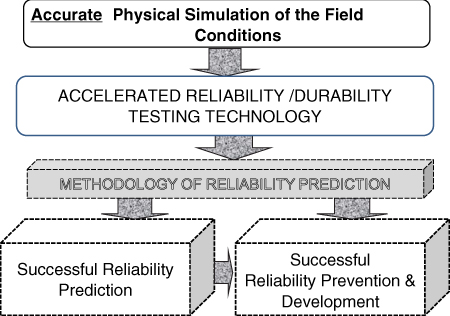
Figure 2.3 Five common steps for successful reliability prediction.
Lev Klyatis created his ideas of successful reliability prediction while working in the USSR, where he developed some of the components, methodology, and tools for this new scientific engineering direction. Then he continued his work in this field after moving to the USA, and which he continues developing to this day, improving the direction, strategy, and continuing the expansion of its implementation.
As was shown in Figure 2.2, this strategy includes two basic components, the details of which were published elsewhere [1–3]. The first component to successful prediction methodology is detailed and described in Section 2.5. The second component was described in detail in Accelerated Reliability and Durability Testing Technology [1]. The basics of this second component will also be described in Chapter.
Figure 2.4 demonstrates the interaction of the three basic groups of real‐world conditions necessary for successful reliability prediction.
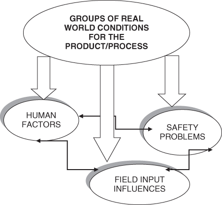
Figure 2.4 Interacted groups of real world conditions for the product/process.
2.4 The Role of Accurate Definitions in Successful Reliability Prediction: Basic Definitions
Accurate definitions of terminology is a key factor in conducting successful reliability prediction. In his previous books this author included some examples of how misunderstanding of definitions can lead to inaccurate prediction [1,3]. Earlier in this chapter, an example of this author's experience with Black & Decker was presented. It was also described [3] how professionals from the Nissan Technical Center considered vibration testing as reliability testing, while not accounting for other significant field input influences. Because these definitions were not properly understood, the results of the testing were not accurate predictors of product performance.
Box 2.1 gives the correct basic definitions that reliability professionals need to know for accurate reliability testing and prediction. Additional definitions can be found in Chapter , which includes the draft standard which has been approved at SAE G‐11 Reliability Committee meetings.
2.5 Successful Reliability Prediction Methodology
The basic methodology for successful reliability prediction includes:
- common criteria for successful prediction of product reliability;
- methodology for selecting representative input regions for accurate simulation of real‐world conditions;
- aspects of successful prediction of product reliability, using manufacturing technology factors and usage conditions;
- building an appropriate testing model for reliability prediction;
- system reliability prediction from testing results of the components.
A depiction of the common scheme of this methodology can be seen in Figure 2.5.
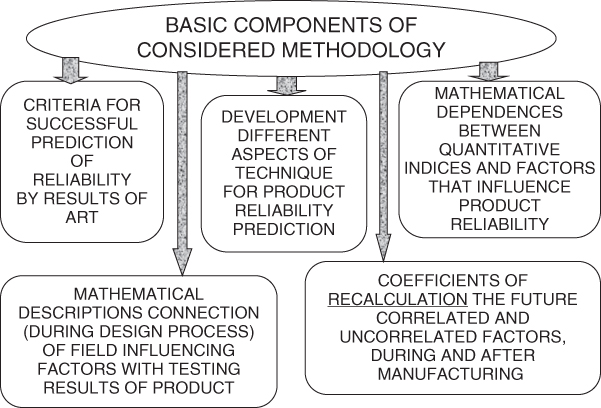
Figure 2.5 Common scheme of methodology for product's reliability successful prediction.
Klyatis and Walls [6] provide further information on the methodology for selecting representative input regions for accurate simulation of real‐world conditions.
2.5.1 Criteria of Successful Reliability Prediction Using Results of Accelerated Reliability Testing
The results of ART are frequently used as a source for obtaining initial information needed to predict the reliability of machinery in field conditions. But for this to be accurate one must be sure that the prediction is correct (if possible, with a given accuracy). The following solution is useful in achieving this goal.
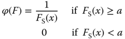
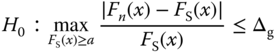
The problem is formulated as follows: there is the system [results of use of the current product in the field] and its model [results of ART/ADT of the same product]. The quality of the system can be estimated by the random value ϕ using the known or unknown law of distribution F S(x). The quality of the model can be estimated by the random value φ using the unknown law of distribution F M. The model of the system will be satisfactory if the measure of divergence between F S and F M is less than a given limit Δg.
After testing the model, one obtains the random variables ϕ
1: ![]() . If one knows F
S(x), by means of
. If one knows F
S(x), by means of ![]() , one needs to check the null hypothesis H
0, which means that the measure of divergence between F
S(x) and F
M(x) is less than Δg. If F
S(x) is unknown, it is necessary also to provide testing of the system. As results of this testing, one obtains realizations of random variables ϕ:
, one needs to check the null hypothesis H
0, which means that the measure of divergence between F
S(x) and F
M(x) is less than Δg. If F
S(x) is unknown, it is necessary also to provide testing of the system. As results of this testing, one obtains realizations of random variables ϕ: ![]() . For the aforementioned two samplings, it is necessary to check the null hypothesis H
0 that the measure of divergence between F
S(x) and F
M(x) is less than the given limit Δg. If the null hypothesis H
0 is rejected, the model needs updating; that is, to look at more accurate ways of simulating the basic mechanism of field conditions use for ART.
. For the aforementioned two samplings, it is necessary to check the null hypothesis H
0 that the measure of divergence between F
S(x) and F
M(x) is less than the given limit Δg. If the null hypothesis H
0 is rejected, the model needs updating; that is, to look at more accurate ways of simulating the basic mechanism of field conditions use for ART.
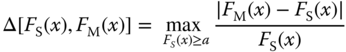
The measure of divergence between F S(x) and F M(x) is functional as estimated by a multifunctional distribution and depends on a competitive (alternate) hypothesis. The practical use of the criteria obtained depends on the type and form of this functional. To obtain exact distributions of statistics on the condition that the null hypothesis H 0 is correct is a complicated and unsolvable problem in the theory of probability. Therefore, here, the upper limits are shown for the statistics and their distributions studied, so the level of values will be increased; that is, explicit discrepancies can be detected. Let us consider the situation when FS(x) is known.
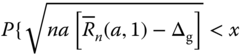
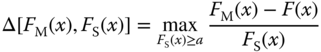
First, we will take as the measure of divergence between the functions of distribution F S(x) and F M(x) the maximum of modulus difference:
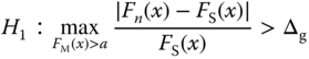
We understand that H 0 is the hypothesis that the modulus of difference between F M(x) and F S(x) is no more than the acceptable level Δg; that is:
where F M(x) is the model (testing conditions) function of distribution.
Against H 0 one checks the competitive hypothesis:
The statistic of the criterion can be given by the formula
Practically, it can be calculated by the following formula:
It is very complicated to find the distribution of this statistic directly [7]. The ![]() as
as ![]() . Therefore, it is necessary to look for the distribution of a random value
. Therefore, it is necessary to look for the distribution of a random value ![]() .
.
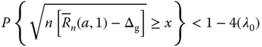
Let us give the upper estimation which can be useful for practical solution of this problem:

If hypothesis H 0 is true, then
Therefore:
or
Here, if F(x) is the probability of work without failure, then n is the number of failures.
Let us denote ![]() as Dn
. This random value
as Dn
. This random value ![]() limited by
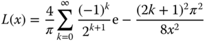
limited by ![]() follows Kolmogorov's law [8]. Therefore:
follows Kolmogorov's law [8]. Therefore:
or

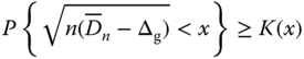
where K(x) is the function of the Kolmogorov distribution.
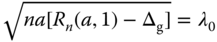
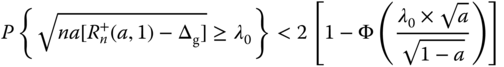
As a result of research, the following is the correct way to use the Kolmogorov criterion. First, one calculates the number ![]() . Then:
. Then:
If the difference ![]() is small, then the probability
is small, then the probability ![]() is also small. This means that an improbable event has occurred, and the divergence between F
n(x) and F
S(x) can be considered as a substantial, rather than a random, character of the values studied and Δg. Therefore, the conclusion is
is also small. This means that an improbable event has occurred, and the divergence between F
n(x) and F
S(x) can be considered as a substantial, rather than a random, character of the values studied and Δg. Therefore, the conclusion is
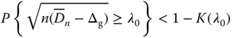
If the level of value of this criterion is higher than ![]() , hypothesis H
0 is rejected. If
, hypothesis H
0 is rejected. If ![]() is large, it does not exactly confirm the hypothesis, but by a small Δg we can practically consider that the testing results do not contradict the hypothesis.
is large, it does not exactly confirm the hypothesis, but by a small Δg we can practically consider that the testing results do not contradict the hypothesis.
Let us take now as a measure of divergence between F S(x) and F M(x) the maximum difference between F S(x) and F M(x) by the Smirnov criterion [9]; that is:
In this case the hypothesis H 0 becomes
The statistic of the criterion is [5]
By analogy with the previous solution, the upper value is
or
The random value ![]() in the limit has a Smirnov distribution; therefore:
in the limit has a Smirnov distribution; therefore:
or
As a result, the following rule for use of the criterion was obtained. First, one calculates the value ![]() . Then
. Then

If ![]() is small, therefore the probability
is small, therefore the probability  is also small, and if we describe it as analogous with the above, then
In consideration of the alternate hypothesis ![]() , everything will be analogous to hypothesis
, everything will be analogous to hypothesis ![]() , because if the minuend and subtrahend exchange places, that will not change the final result.
, because if the minuend and subtrahend exchange places, that will not change the final result.
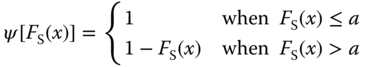
Second, let us consider checking the hypothesis H
0 by using the alternate hypothesis ![]() with only the weight function
with only the weight function
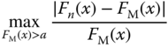
Let us take as a measure of divergence between F S(x) and F M(x)
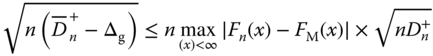
The statistics of the criterion can be expressed by
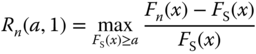
For this practical calculation the following formula can be used:
As stated earlier, the upper value for this statistic was found to be

Hypotheses H 0 and H 1 then become
We obtain Equation 2.2, because
is a statistic of ![]() .
.
Therefore, the random value ![]() , limited by
, limited by ![]() , follows the law of distribution [7]:
, follows the law of distribution [7]:
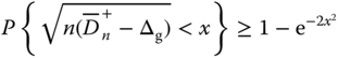
From here
or
So, we obtained the Klyatis criteria that are modifications of the Kolmogorov and Smirnov criteria.
There is the following rule for using Klyatis's criteria:
- One calculates the actual number
 .
. - In that case:

- If
 is small, then the probability
 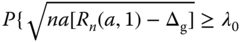 will also be small. This means that the difference between Fn
(x) and F
S(x) is significant.
will also be small. This means that the difference between Fn
(x) and F
S(x) is significant.
Then we will take the maximum difference as a measure of divergence:
This problem can also be solved by the method analogous to the previous solution. The rule of use of this criterion is as follows. One calculates the actual number
Then
If ![]() is small, it means that hypothesis H
0 is rejected, and then by analogy with previous solutions the same applies to the competitive hypothesis H
1
.
is small, it means that hypothesis H
0 is rejected, and then by analogy with previous solutions the same applies to the competitive hypothesis H
1
.
All are analogous with weight function
Let us now consider the variant when F
S(x) is unknown. In this case one provides an ART of the prediction subject. As a result, one obtains realizations of the random value ϕ of system reliability, ![]() , and can use these realizations to build functions of the distribution Fm
(x). By means of the functions of distribution Fn
(x) and Fm
(x), it is necessary to establish whether the random value studied relates to one class or not; that is, will the divergence between the actual functions of distribution Fn
(x) and F
S(x), by a certain measure, be less or more than the given tolerance Δg.
, and can use these realizations to build functions of the distribution Fm
(x). By means of the functions of distribution Fn
(x) and Fm
(x), it is necessary to establish whether the random value studied relates to one class or not; that is, will the divergence between the actual functions of distribution Fn
(x) and F
S(x), by a certain measure, be less or more than the given tolerance Δg.
Let us take the measure of divergence in the Smirnov criterion as a measure of divergence between functions of distribution [9]:
In this case the null hypothesis H 0 looks like
The alternative hypothesis ![]() looks like
looks like
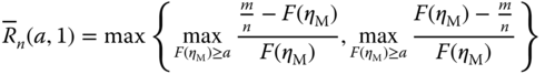
The statistic of the criterion can be expressed by the following formula:
Its upper estimation

If hypothesis H 0 is true, then
where
Statistics ![]() and
and ![]() , as was shown earlier, have equal distributions. Therefore:
, as was shown earlier, have equal distributions. Therefore:
Therefore:

Let n and m approach infinity, so that ![]() . Then
. Then

Let us denote the random variable ![]() through V
2. V has a Smirnov function of distribution
through V
2. V has a Smirnov function of distribution ![]() . Then from the assumption that m and n are large enough, this solution has already been published by Klyatis [1,2]. As a result, we obtain the following rule of criterion use.
. Then from the assumption that m and n are large enough, this solution has already been published by Klyatis [1,2]. As a result, we obtain the following rule of criterion use.
To calculate the actual number

where n is number of failures during ART/ADT and m is the number of failures in the field.
Therefore:
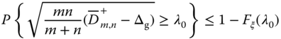
If ![]() is small, the hypothesis H
0 is rejected by analogy with the previous calculations. In this case
is small, the hypothesis H
0 is rejected by analogy with the previous calculations. In this case ![]() if
if ![]() or
or ![]() .
.
If we take as a measure of divergence between distributions of functions a functional
and make the actions analogous to previously, then we obtain the rule of use for the criterion in the following form. First, we calculate the following number:
Then

If ![]() is small, it means that the hypothesis H
0 is rejected, and then is analogous to previous actions.
is small, it means that the hypothesis H
0 is rejected, and then is analogous to previous actions.
For finding the distribution of random variable k, one can use special dependences, where

in the function of Kolmogorov's distribution
In conclusion:
- The engineering version of the solution obtained is that the upper estimation of the statistical criteria of correspondence, for some measures between the functions of distribution of studied reliability characteristics were created in ART conditions and in field conditions. This can be useful for practical reliability prediction for industry as well as for solving other engineering problems (accelerated reliability development and improvement, etc.).
- The mathematical version of the solution obtained is that approximate Klyatis criteria as modifications of Smirnov's and Kolmogorov's criteria by divergence (
 ) were obtained for comparison of two empirical functions of distribution by measurement of the Smirnov divergence
and the Kolmogorov divergence
In the Smirnov criterion by zero hypothesis, we have
By the competitive hypothesis, we have
If ![]() , we have the Smirnov criterion. An analogous situation applies for the Kolmogorov criterion. The difference between the two versions is that in the measure using the Klyatis modification of the Smirnov criterion one takes into account only those regions (the oscillograms of loadings, etc.) where
, we have the Smirnov criterion. An analogous situation applies for the Kolmogorov criterion. The difference between the two versions is that in the measure using the Klyatis modification of the Smirnov criterion one takes into account only those regions (the oscillograms of loadings, etc.) where ![]() and one looks for maximum differences only for them.
and one looks for maximum differences only for them.
In measuring with the Klyatis modification of Kolmogorov's criterion one takes into account the maximum differences for all regions by modulus. The consideration of both criteria makes sense, because Smirnov's criterion is easier to calculate, but does not give the full picture of divergences between F S(x) and F M(x); Kolmogorov's criterion gives a fuller picture of the above divergence, but is more complicated in calculation.
Therefore, the choice of the better criterion for a specific situation must be decided according to the specific conditions of the problem to be solved.
Let us show the solution obtained by a practical example. In the field, the details for ![]() failures of car transmissions were obtained. After ART/ADT, 95 failures were obtained:
failures of car transmissions were obtained. After ART/ADT, 95 failures were obtained: ![]() ,
, ![]() .
.
In the field one builds the empirical function of distribution of the time to failures Fm (x) by the intervals between failures, and one builds by intervals between failures during ART/ADT of the function of distribution time to failures F M(x). As we can see, this is the last variant to be considered
If we align the graph F
M(x) (Figure 2.1) and the graph ![]() , we will find the maximum difference between F
M(x) and Fm
(x). For this goal we can draw the graph Fm
(x) on transparent paper and it is simple to find the maximum difference
, we will find the maximum difference between F
M(x) and Fm
(x). For this goal we can draw the graph Fm
(x) on transparent paper and it is simple to find the maximum difference ![]() . In correspondence with Ventcel [10], we have
. In correspondence with Ventcel [10], we have ![]() :
:
and therefore
After substitution of ![]() , we obtain
, we obtain ![]() . Therefore,
. Therefore, ![]() . So,
. So, ![]() is not small and the hypothesis H
0 can be accepted. Therefore, the divergence between actual functions of distribution of time to failures of the aforementioned test subject (e.g., car transmission) details for the car tested in field conditions and in ART/ADT conditions by Smirnov's measure is within the given limit
is not small and the hypothesis H
0 can be accepted. Therefore, the divergence between actual functions of distribution of time to failures of the aforementioned test subject (e.g., car transmission) details for the car tested in field conditions and in ART/ADT conditions by Smirnov's measure is within the given limit ![]() (Figure 2.6)
. This gives the possibility for successful prediction of reliability of the car transmissions using the results of this testing.
(Figure 2.6)
. This gives the possibility for successful prediction of reliability of the car transmissions using the results of this testing.

Figure 2.6 Evaluation of the correspondence between functions of distribution of the time to failure of a car trailer's transmission details in the field and in the ART/ADT conditions.
2.5.2 Development of Techniques for Product Reliability Prediction Using Accelerated Reliability Testing Results
This section will address the problem of solving the successful prediction of product reliability taking into account the effects of reliability with complex input factors.
The typical practice in engineering is to test a small sample number (from five to ten test specimens of each component) with two to five possible failures deemed as acceptable. Usually, it is assumed that the failures of the system components are statistically independent.
This proposed approach is very flexible and useful for many different types of products, including electronic, electromechanical, mechanical, and others.
2.5.2.1 Basic Concepts of Reliability Prediction
As was mentioned earlier in this book, in order for reliability prediction to be useful, it must be based on the appropriate methodology, techniques, and equipment to assure accurate initial information for the prediction.
The methodology was partially considered earlier.
ART/ADT can give this information if one follows the successive step‐by‐step technology described in this book.
The basic concept of successful reliability prediction consists of the following basic steps:
- Building an accurate model of real‐time performance.
- Using the model for testing the product and studying the degradation mechanism over time and comparing model degradation with the real‐life degradation mechanism of the product. If the degradation mechanism differs by more than a fixed defined limit, one must improve the model's real‐time performance.
- Making real‐time performance forecasts for reliability prediction using these testing results as initial information.
Each step can be performed in different ways, but reliability can only the predicted accurately if the researchers and engineers use this concept.
Step 1 can only be performed if one understands that real‐life reliability of the product depends on a combination of different interacted input influences, such as is shown in Chapter . The simulation of input influences must be as complicated as they are in real‐life conditions. For example, for a mobile product one needs to use multi‐axis vibration in combination with multi‐environmental and other factor testing.
In order to solve step 2 one has to understand the degradation mechanism of the product and the parameters affecting this mechanism. The causes of the product's degradation mechanism are included in the data, for example the data must include, the electrical, mechanical, chemical, thermal, and radiation effects. And some of the parameters of the mechanical degradation include deformation, crack, wear, creep, and so on. In real life, different processes of degradation may be acting simultaneously and in combination.
Therefore, ART must also include the simultaneous combination of different types of testing (environmental, electrical, vibration, etc.), with the assumption that the failures are statistically related to these combined factors. The degradation mechanism of the product during ART/ADT must be closely similar to the mechanism that occurs in real life.
In order to solve step 3 of this reliability prediction technique, all pertinent aspects must be considered, including both manufacturing and field conditions.
2.5.2.2 Prediction of the Reliability Function without Finding the Accurate Analytical or Graphical Form of the Failures' Distribution Law
The problem was solved for two types of conditions: (a) prediction consisting of point expressions of reliability function of the system elements; (b) prediction of the reliability functions of the system with predetermined accuracy and confidence area [11].
Problem (a) can be solved with grapho‐analytical methods on the basis of failure hazard or frequency if we have the graph f(t) of the empirical frequency of failures; then, guided by the failure frequency graph, one can discover the reliability function:

where  is the area under the curve f(t) that was obtained as a result of ART.
The reliability function of a system which consists of different components (details) is:
For example, as a result accelerated testing of belts ![]() , the area is
, the area is ![]() , and probability
, and probability ![]() .
.
In variant (b) one needs to calculate the accumulated frequency function and the values of the confidence coefficient found in the equations:


and evaluate the curves that are limited to the upper and lower confidence areas. In Equations 2.6 and 2.7, ![]() is the probability that, based on an event, there will be in n independent experiments m times. The values of
is the probability that, based on an event, there will be in n independent experiments m times. The values of ![]() and
and ![]() are found in the tables of the books on the theory of probability if the confidence coefficient is
are found in the tables of the books on the theory of probability if the confidence coefficient is ![]() or
or ![]() .
.
2.5.2.3 Prediction Using Mathematical Models Without Indication of the Dependence Between Product Reliability and Different Factors of Manufacturing and Field Usage
These factors (influences) should be evaluated as the results of ART/ADT. The solution of this problem is possible using mathematical models which best describe the dependence between the reliability and the series of factors shown above:
where θ is the number of all factors, n is the number of reliability indexes which most completely characterize the ith model of the product, ![]() is the function that gives the possibility of finding the optimum value of these functions indexes, by changing the level of factors influencing the products' reliability. A large amount of statistical data is necessary to build this function, which can be obtained by experiments with fixed values of factors for estimation of reliability indexes.
is the function that gives the possibility of finding the optimum value of these functions indexes, by changing the level of factors influencing the products' reliability. A large amount of statistical data is necessary to build this function, which can be obtained by experiments with fixed values of factors for estimation of reliability indexes.
This is a difficult problem that requires a large expenditure of resources for its solution. Prediction of reliability indexes for a product which will be manufactured in the future is more readily obtained by results of ART/ADT of its early specimens. In this case, one part of the input influences (mechanical, environmental, etc.) can be used to obtain results of product ART/ADT. Another part (influences of manufacturing specifics, conditions of operator specifics, etc.) must be taken into account when studying the results of mathematical modeling.
In this case, the connection between evaluation of ![]() of the τth quantified reliability index of the ith model of product in the jth conduction of use, which needs of prediction, and the mean value of this index
of the τth quantified reliability index of the ith model of product in the jth conduction of use, which needs of prediction, and the mean value of this index ![]() , which can be obtained as a result of accelerated testing of μ specimens of the product, is described with functional dependence
, which can be obtained as a result of accelerated testing of μ specimens of the product, is described with functional dependence
where ![]() and
and ![]() are the most important lack of correlated common factors of manufacture and in the field;
are the most important lack of correlated common factors of manufacture and in the field; ![]() and
and ![]() are unknown parameters of the mathematical model in Equation 2.9 which are characterized by the group of manufacture and field factors
are unknown parameters of the mathematical model in Equation 2.9 which are characterized by the group of manufacture and field factors
![]() and
and ![]() are the numbers of the most important lack of correlated common factors of manufacturing and the field.
are the numbers of the most important lack of correlated common factors of manufacturing and the field.
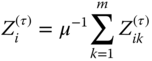
The mean value ![]() , which is a result of ART/ADT of μ specimens (usually not more than two or three specimens), can be evaluated as
, which is a result of ART/ADT of μ specimens (usually not more than two or three specimens), can be evaluated as
The results of the aforementioned testing are independent of factors that cannot be simulated in the laboratory. Therefore, in the model in Equation 2.9 the variable can be divided into
where ![]() are the recalculated coefficients of the quantitative values' quantitative index of future product reliability concerning the indexes of means indexes which have been obtained by ART of specimens.
are the recalculated coefficients of the quantitative values' quantitative index of future product reliability concerning the indexes of means indexes which have been obtained by ART of specimens.
These coefficients depend on manufacturing and field conditions, which themselves are time dependent and contain unknown parameter values. The values of these coefficients are different for different products and different indexes of reliability. This is because the levels of the most important factors of manufacturing by different companies and in different field conditions are not the same. The values of recounting coefficients may be more or less than one for different reliability indexes. Therefore, the coefficients are functionals:
where ![]() is the function which evaluates the level of influence on the product reliability of the basic lack of correlated generalized factors of the field and manufacturing conditions. The most important factors are characterized by ponderable levels P and Q and actual levels Xi
and Yi
.
is the function which evaluates the level of influence on the product reliability of the basic lack of correlated generalized factors of the field and manufacturing conditions. The most important factors are characterized by ponderable levels P and Q and actual levels Xi
and Yi
.
Let us consider the function of the impact of the statistical problem of product reliability prediction if we take into account the weak dependence of these factors on time:
where ![]() and
and ![]() are means of specific ponderabilities of the values of the actual levels and the mean of the ponderabilities of manufacturing and field are the most important factors. The study of reliability prediction and the dependence on specific manufacturing and field conditions (operating conditions) of different companies will be discussed later in this book.
are means of specific ponderabilities of the values of the actual levels and the mean of the ponderabilities of manufacturing and field are the most important factors. The study of reliability prediction and the dependence on specific manufacturing and field conditions (operating conditions) of different companies will be discussed later in this book.
Let us build a specific influence function which can help to determine:
- the level of the combined impact of all the most important lack of correlated and generalized factors of manufacture and field action;
- the level of impact of individual groups of factors (the group of manufacturing factors and group of field factors) on product reliability;
- the level of impacts of individual factors of the group of the most important factors.
The functions ![]() for all quantities of reliability indexes appear to be equal, because the form of influence for different factors of manufacturing and field is identical for all reliability indexes. But the values for any reliability indexes may be different. The difference should be taken into account with unknown parameters
for all quantities of reliability indexes appear to be equal, because the form of influence for different factors of manufacturing and field is identical for all reliability indexes. But the values for any reliability indexes may be different. The difference should be taken into account with unknown parameters ![]() and
and ![]() which have specific values for each quantity of reliability indexes, for each model of product, each set of field conditions, and for each product of the company.
which have specific values for each quantity of reliability indexes, for each model of product, each set of field conditions, and for each product of the company.
Let us give for this function the following requirements:
- it must always be positive;
- the maximum value must be less than or equal to 1.00 to give the possibility of simplifying the mathematical model by calculating the functional in Equation 2.14.
In addition, the practical requirement is that the reliability of the specimen used for the testing during the design process is usually higher than after manufacturing of this product, and the time for maintenance is usually less.
Therefore, the coefficients of recalculating the mean time to failure and the mean time of maintenance are characterized by the following dependence:
If we take into account the lack of correlation of separate factors and groups of factors, we obtain the following equation (after manipulation):

where ![]() and
and ![]() are normalized coefficients which relate to the mean specific ponderabilities bn
and br
of different groups of factors. For this, our research gives the following results:
are normalized coefficients which relate to the mean specific ponderabilities bn
and br
of different groups of factors. For this, our research gives the following results: ![]() and
and ![]() .
.
The input of normalized coefficients is necessary, because if ponderability of group of factors (or a separate factor) is greater, the decrease in the product reliability which depends on this group (factor) must be more. It means that the quantity of influence function must be less.
By analogy, normalized coefficients αk and βk were included:

One can find the unknown parameters ![]() and
and ![]() for prototypes, because they cannot be determined for future or modernized products. For example,
for prototypes, because they cannot be determined for future or modernized products. For example, ![]() can be evaluated if we compare the τth index of reliability of the ith model of the product which is obtained as a result of ART of μ specimens and as a result of studying of υ specimens in the field.
can be evaluated if we compare the τth index of reliability of the ith model of the product which is obtained as a result of ART of μ specimens and as a result of studying of υ specimens in the field.
Unknown parameter ![]() is evaluated by sum of parameters
is evaluated by sum of parameters ![]() .
.
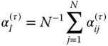
where N is the number of regions where the previous model is used.
Therefore, for prediction of time to failures the following equation can be recommended:
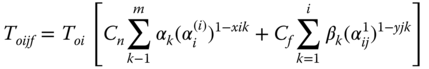
where Toi is the mean time to failure. It is obtained a result of ART of μ specimens.
2.5.2.4 Practical Example
As a result of short field testing of new self‐propelled spraying machines Ro Gator 554 and John Deere 6500, the mean time to failure and mean time for maintenance were obtained (Table 2.1).
Table 2.1 The results of short field testing of prototypes of self‐propelled spraying machines.
| Prototype of Ro Gator 554 | Prototype of John Deere 6500 | |||
| Index | Prestige Farms, Clinton (NC) | Continental Grain Co. (NY) | Prestige Farms, Clinton (NC) | Continental Grain Co. (NY) |
| Mean time to failure (h) | 104 | 73.80 | 104 | 171.10 |
Now let us take as the prototypes the Finn T‐90 and T‐120. The results of field testing of four specimens of these machines can be seen in Table 2.2.
Table 2.2 Testing results of prototypes of the studied machines.
| Conditions of machines used, No. of model | Time to failure (h) |
| Murphy Family Farm | |
| Finn T‐90 | |
| No. 287 | 21.9 |
| No. 261 | 29.04 |
| No. 290 | 53.62 |
| No. 291 | 47.81 |
| Mean | 37.92 |
| T‐120 | |
| No. 059 | 49.32 |
| No. 030 | 48.22 |
| No. 063 | 56.2 |
| No.218 | 67.41 |
| Mean | 58.37 |
| Caroll & Foods | |
| Finn T‐90 | |
| No. 316 | 40.92 |
| No. 358 | 1.72 |
| No. 1001 | 37.67 |
| No. 1005 | 5871 |
| Mean | 39.63 |
| T‐120 | |
| No. 714 | 58.72 |
| No. 1105 | 80.54 |
| No. 4516 | 62.98 |
| Mean | 67.41 |
The values of normalized coefficients αk , βk , and qk were obtained in correspondence with the mean specific ponderabilities of the most important manufacturing and field factors, using Equation 2.16 (Table 2.3).
Table 2.3 Normalized coefficients corresponding with the most important manufacturing and field factors.
| Normalized coefficient | 1 | 1 | 3 | 4 | 5 | 6 |
| Pk | 0.2325 | 0.2225 | 0.2125 | 0.175 | 0.1575 | — |
| αk | 0.1920 | 0.1940 | 0.1970 | 0.206 | 0.2110 | — |
| qk | 0.2325 | 0.2250 | 0.2075 | 0.130 | 0.1125 | 0.0925 |
| βk | 0.1540 | 0.1550 | 0.1590 | 0.174 | 0.1780 | 0.1820 |
The unknown parameters of α were obtained using Equation 2.8 and Tables 2.2, 2.3, , and 2.4.
Table 2.4 Unknown parameters αi and αij .
| T‐90 | T‐120 | |||||
| Murphy Family Farms | Caroll & Foods | Prestige Farms | Murphy Family Farms | Caroll & Foods | Prestige Farms | |
|
|
0.42 | 0.47 | 0.445 | 0.19 | 0.23 | 0.21 |
|
|
0.45 | 0.75 | 0.60 | 0.56 | 0.80 | 0.68 |
The coefficients of recalculating for new machines were obtained (Table 2.5) using the equations and Tables 2.3 and 2.4.
Table 2.5 Coefficient of recalculating for the machines studied.
| Ro Gator 554 | John Deere 6500 | |||
| Prestige Farms | Continental Grain Co. | Prestige Farms | Continental Grain Co. | |
| Mean time to failure (h) | 0.64 | 0.66 | 0.43 | 0.45 |
The mean time to failure of the new machines Ro Gator 554 and John Deere 6500 were predicted for when they will be manufactured by series, using Equations 2.22) and (2.23) and Tables 2.1 and 2.5 (Table 2.6).
Table 2.6 Predicted mean time to failure.
| Ro Gator 554 | John Deere 6500 | |||
| Prestige Farms | Continental Grain Co. | Prestige Farms | Continental Grain Co. | |
| Mein time to failure (h) | 57.12 | 59.01 | 59.67 | 62.61 |
If one wants to predict system reliability from accelerated testing results of the components, one can use the solution, which was published elsewhere [12].
References
- 1 Klyatis L. (2012). Accelerated Reliability and Durability Testing Technology. John Wiley & Sons.
- 2 Klyatis L, Klyatis E. (2006). Accelerated Quality and Reliability Solutions. Elsevier.
- 3 Klyatis L. (2016). Successful Prediction of Product Performance. Quality, Reliability, Durability, Safety, Maintainability, Life Cycle Cost, Profit, and Other Components. SAE International, Warrendale, PA.
- 4 Klyatis LM. (2017). Why separate simulation of input influences for accelerated reliability and durability testing is not effective? In SAE 2017 World Congress, Detroit, paper 2017‐01‐0276.
- 5 Klyatis L, Klyatis E. (2002). Successful Accelerated Testing. Mir Collection, New York.
- 6 Klyatis L, Walls L. (2004). A methodology for selecting representative input regions for accelerated testing. Quality Engineering 16(3): 369–375.
- 7 Van der Waerden BL. (1956). Mathematical Statistics with Engineering Annexes. Springer (in German).
- 8 Kolmogorov AN. (1941). Interpolation and extrapolation of stationary random sequences. Izvestiya Akademii Nauk SSSR: Seriya Matematicheskaya 5: 3–14.
- 9 Smirnov NV. (1944) Approximation of distribution laws of random variables by empirical data. Uspekhi Matematicheskikh Nauk 10: 179–206.
- 10 Ventcel ES. (1966). Theory of Probability. Vysshaya Shkola, Moscow.
- 11 Klyatis LM. (1985). Accelerated Evaluation of Farm Machinery. Agropromisdat, Moscow.
- 12 Klyatis LM, Teskin OI, Fulton JW. (2000) Multi‐variate Weibull model for predicting system reliability, from testing results of the components. In The International Symposium of Product Quality and Integrity (RAMS) Proceedings, Los Angeles, CA, January 24–27, pp. 144–149.
Exercises
- 2.1 Describe what happened during Dr. Klyatis's consulting work in improving testing for Black & Decker Company.
- 2.2 How did Dr. Klyatis continue developing the system he had created earlier for successful reliability prediction for industry after he came to the USA?
- 2.3 Provide some of the reasons why many publications in reliability prediction could not be successfully used by industry?
- 2.4 How many basic steps are needed to implement successful reliability prediction? Describe them.
- 2.5 Why are proper definitions so important in reliability prediction?
- 2.6 Describe the definition of “accurate system reliability prediction.”
- 2.7 Describe the definition of “correct accelerated reliability testing.”
- 2.8 What basic components need to be simulated for accelerated corrosion testing?
- 2.9 What basic components are needed to simulate accelerated vibration testing?
- 2.10 What is the difference between what is commonly referred to as vibration testing and accelerated reliability (or durability) testing?
- 2.11 What components should be included in the methodology of reliability prediction?
- 2.12 What components consists of common scheme of methodology for products successful reliability prediction?
- 2.13 Why is it that many published methodologies cannot be used successfully by industry?
- 2.14 Consider the basic meaning of criteria of successful reliability prediction using results of accelerated reliability testing.
- 2.15 Explain the difference between Kolmogorov and Smirnov criteria?
- 2.16 What is difference between Klyatis criteria and Kolmogorov and Smirnov criteria?
- 2.17 What is the rule of Klyatis criteria usage?
- 2.18 What are the basic concepts of reliability prediction using accelerated reliability or durability testing as a source of initial information for prediction calculation?
- 2.19 What is the basic essence of using the prediction reliability function without finding accurate analytical or graphical forms of the failure distribution law?
- 2.20 What is the basic essence of predicting with use of the mathematical models without indication of the dependence between product reliability and the different factors of manufacturing and field usage.
- 2.21 Show the common scheme of successful reliability prediction for industry.
- 2.22 Demonstrate five common steps for successful reliability prediction. Describe them.
- 2.23 Show how the interacted groups of real‐world conditions for the product/process need to be taken into account for successful reliability prediction.