
6
A Real‐Time Information‐Based Demand‐Side Management System
Demand response is a feature to be achieved in the smart grid. In this chapter, we study a few mechanisms to demonstrate the enhanced efficiency in the smart grid with demand response.
6.1 Background and Related Work
6.1.1 Background
Demand response (DR), also known as demand‐side management system [27–29], utilizes real‐time information in order to let the power grid generate and consume energy more efficiently while reducing fuel waste. A DR system is widely agreed to be effective at reducing the peak‐to‐average ratio (PAR) of energy consumption [28, 29, 98]. This improvement helps power suppliers reduce the extra fuel costs caused by dramatic and unpredictable margin fluctuations in power generation. Burning less fuel also helps reduce emission of greenhouse gas from those power generators. Moreover, since the control center gets the energy consumption schedule beforehand [83, 99–101], renewable sources such as photovoltaics (PV) and wind turbines, which are less stable and less controllable compared than conventional power generators, can support the power grid more efficiently. A higher proportion of such renewable sources will further reduce the burning of fuel by conventional power generators.
In this chapter, we first propose a centralized optimization problem ![]() in order to reduce PAR to its minimum. Although a minimum PAR is obviously beneficial to the environment, it motivates neither power suppliers nor customers. Power suppliers especially must deploy and maintain a more complicated cyber physical system than what AMI can offer to gather and distribute a huge amount of detailed information in real time. Therefore, a monetary incentive is needed to motivate power suppliers. Another centralized optimization problem
in order to reduce PAR to its minimum. Although a minimum PAR is obviously beneficial to the environment, it motivates neither power suppliers nor customers. Power suppliers especially must deploy and maintain a more complicated cyber physical system than what AMI can offer to gather and distribute a huge amount of detailed information in real time. Therefore, a monetary incentive is needed to motivate power suppliers. Another centralized optimization problem ![]() is then proposed to reduce the total cost of energy generation cost to power suppliers. Although power suppliers may be willing to adopt the DR system based on
is then proposed to reduce the total cost of energy generation cost to power suppliers. Although power suppliers may be willing to adopt the DR system based on ![]() , it is based on direct load control (DLC) [99, 102, 103], which could be defective. In terms of communications, even if the massive centralized problem can be solved efficiently, the transmission overhead will create a huge burden on the communication network and require more advanced technical upgrades as well as more frequent maintenance. Moreover, customers could be reluctant to adopt such a DR system for two reasons. One reason is that the control center takes over the energy consumption scheduling from customers with no clear incentive for them to do so. The other reason is that DLC requires too much private information from customers.
, it is based on direct load control (DLC) [99, 102, 103], which could be defective. In terms of communications, even if the massive centralized problem can be solved efficiently, the transmission overhead will create a huge burden on the communication network and require more advanced technical upgrades as well as more frequent maintenance. Moreover, customers could be reluctant to adopt such a DR system for two reasons. One reason is that the control center takes over the energy consumption scheduling from customers with no clear incentive for them to do so. The other reason is that DLC requires too much private information from customers.
To tackle those issues, we must have a DR system that clearly benefits customers, protects their privacy, and requires much less real‐time information exchange compared with ![]() or
or ![]() . We formulate a game with two approaches based on smart pricing, which is another major technique applied to the DR system. In one approach, customers get to compute the dynamic price based on their own load schedule, with the total load of the power grid given. In the other approach, the control center computes the price based on the total load of the power grid, and customers get that fixed price schedule that will not be affected by their local scheduling load. In either game theoretical approach, the payoff functions lead customer to more energy cost savings. Therefore, customers are motivated to adopt this DR system. In addition, customers reserve the right to control their power consumption, and by doing so, they keep their information private by submitting only the energy consumption schedule, which is always requested even in the traditional power grid. Moreover, since most of the calculation is performed locally at the customer side, the approaches are mostly distributed instead of centralized. The distributed game theoretical approach largely relieves the transmission overhead. More importantly, we prove that all
. We formulate a game with two approaches based on smart pricing, which is another major technique applied to the DR system. In one approach, customers get to compute the dynamic price based on their own load schedule, with the total load of the power grid given. In the other approach, the control center computes the price based on the total load of the power grid, and customers get that fixed price schedule that will not be affected by their local scheduling load. In either game theoretical approach, the payoff functions lead customer to more energy cost savings. Therefore, customers are motivated to adopt this DR system. In addition, customers reserve the right to control their power consumption, and by doing so, they keep their information private by submitting only the energy consumption schedule, which is always requested even in the traditional power grid. Moreover, since most of the calculation is performed locally at the customer side, the approaches are mostly distributed instead of centralized. The distributed game theoretical approach largely relieves the transmission overhead. More importantly, we prove that all ![]() ,
, ![]() , and the game theoretical approach with locally computed dynamic smart pricing lead to the same minimum PAR. Therefore, while all parties get enough motivation to participate, the DR system can be deployed in a distributed way.
, and the game theoretical approach with locally computed dynamic smart pricing lead to the same minimum PAR. Therefore, while all parties get enough motivation to participate, the DR system can be deployed in a distributed way.
6.1.2 Related Work
DR in the smart grid has been studied by many researchers recently [27–29, 83, 98–101, 104–106]. However, most of the works focus on one of the parties (e.g. power suppliers when applying DLC or customers when adopting smart pricing) in the system only, without clarifying why others were overlooked. The game theoretical approach and smart pricing have also been widely adopted in most of the studies as efficient approaches. The works most relevant to this paper includes [28, 29, 99]. The authors of [28] proposed a noncooperative game played among residential customers, and a two‐stage Stackelberg game theoretical approach where power suppliers as the leaders tend to maximize their profits and customers as the followers tend to minimize their costs. Since [28] mostly targeted residential customers, the benefits for other parties in the system were not clearly stated, and an impractical situation where the total load goes negative was carefully avoided. In [29], the authors proposed an efficient game theoretical approach for residential customers without a storage unit based on dynamic smart pricing to reduce the PAR. While computational efficiency was demonstrated, the global optimal PAR was not guaranteed by the distributed approach. The authors of [99] are among of the first to minimize PAR by using a distributed game theoretical approach among customers. Similarly, the consideration of a storage unit was reserved for their future work, and the global optimal PAR was not guaranteed.
We summarize the main contributions as follows:
- In order to benefit the entire society and the environment, we propose a DLC‐based centralized approach to minimizing PAR.
- In order to show the benefits to the power suppliers, we propose another DLC‐based centralized approach that minimizes the cost of power generation, and the power generation cost model considers all sources, including conventional, nonexpanding green energy, and expanding renewable energy sources.
- In order to motivate customers to adopt the DR system and protect their privacy, we propose smart pricing based game theoretical approaches that can maximize savings for customers adopting such a DR system. The game theoretical approaches are mostly distributed, and thus they alleviate the communication burden of the network.
- We prove that the proposed DLC‐based approach and one of the smart‐pricing‐based distributed game theoretical approaches yield the same optimal solution (minimum PAR); therefore the distributed game theoretical approach can be applied in real situations while all parties observe clear benefits from the DR system.
- We provide extensive numerical analysis and simulation results to demonstrate our analysis. We also compare several distributed approaches in order to find the best way to deploy the DR system.
6.2 System Model
6.2.1 The Demand‐Side Power Management System
The DR system under consideration mainly consists of three parts: the control center, power suppliers, and customers, as illustrated in Figure 6.1. Power generators include all major types, from fuel‐consuming conventional power generators to renewable power generators. For simplicity, a micro grid that can be attached to or detached from the power grid is not considered, and customers do not have power generators. The control center is mainly responsible for power distribution. It also gathers data (e.g. energy consumption) and distributes control information (e.g. price, tariff, and emergency control signal). The information is available because of a two‐way communication network in the DR system. At each customer site, there is a smart meter that is responsible for reporting the power consumption and possible scheduling to the control center through the communication network. It is also responsible for receiving price, tariff, and other control information from the control center.

Figure 6.1 Demand‐side power management system.
According to [107], major customers in the United States include residential, business, and industrial ones as shown in Figure 6.2. Those customers have different characteristics when consuming electric energy. For example, residential customers may consume power mostly from afternoon through midnight, business customers consume energy mostly during office hours, while industrial customers may have a longer peak consumption schedule because of continuous shifts by different work groups. The deployment of energy storage units and the use of plug‐in hybrid vehicles (PHEV) are increasing rapidly. Such devices/appliances will increase energy consumption and change the current peak time schedule. For example, it is reasonable to assume that most customers will charge their PHEV during the night. For simplicity, the PHEV is considered as a hybrid of a normal energy‐consuming appliance and an energy storage unit in the studied DR system.
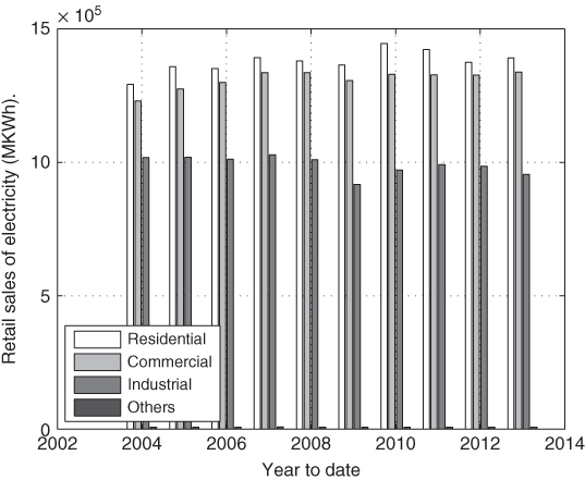
Figure 6.2 Power sale to the customers in United States.
6.2.2 Mathematical Modeling
Table 6.1 lists the key notations of sets and variables we use throughout the rest of this chapter. Let ![]() be the set of all customers, where
be the set of all customers, where ![]() is the total number of customers. Although the DR system can be modeled for any arbitrary time period to satisfy the assumptions, we consider a daily model in this work without loss of generality. Let one day be divided into several uniform time intervals, denoted as
is the total number of customers. Although the DR system can be modeled for any arbitrary time period to satisfy the assumptions, we consider a daily model in this work without loss of generality. Let one day be divided into several uniform time intervals, denoted as ![]() .
.
Table 6.1 Key sets and variables.
| Global | |
| set of customers | |
| set of time intervals | |
| daily energy consumption scheduling | |
| set of total cost for each time interval | |
| set of unit price for each time interval | |
| Local (for customer | |
| set of appliances | |
| daily energy scheduling set of | |
| Energy requirement set | |
| on/off operating scheduling set of | |
| discharging scheduling of storage unit | |
| charging scheduling of storage unit | |
| daily energy consumption scheduling set | |
Each customer ![]() has a set of appliances
has a set of appliances ![]() , where
, where ![]() . Each appliance (e.g.
. Each appliance (e.g. ![]() ) has a daily energy consumption scheduling set
) has a daily energy consumption scheduling set ![]() , which records the energy needed or consumed during each time interval. Moreover, each appliance
, which records the energy needed or consumed during each time interval. Moreover, each appliance ![]() also has a predetermined energy requirement
also has a predetermined energy requirement ![]() for a time period (assuming one day for simplicity). Therefore, for
for a time period (assuming one day for simplicity). Therefore, for ![]() , it must satisfy
, it must satisfy
where ![]() is a column vector of
is a column vector of ![]() and
and ![]() calculates the transposition. Appliance
calculates the transposition. Appliance ![]() has an on/off operating scheduling set
has an on/off operating scheduling set ![]() , where 1 indicates that
, where 1 indicates that ![]() is allowed to operate, whereas 0 indicates an off status for
is allowed to operate, whereas 0 indicates an off status for ![]() . The on/off operating schedule can model the operating status more precisely than the model using an operating time period, which is more widely adopted [28, 29, 99]. For example, with an on/off operating schedule, it is possible to model a two‐hour pause in an air‐conditioning (AC) system. However, if it is modeled by the operating time period, the time period must be divided into three corelated sessions with extra constraints. With the on/off operating scheduling set
. The on/off operating schedule can model the operating status more precisely than the model using an operating time period, which is more widely adopted [28, 29, 99]. For example, with an on/off operating schedule, it is possible to model a two‐hour pause in an air‐conditioning (AC) system. However, if it is modeled by the operating time period, the time period must be divided into three corelated sessions with extra constraints. With the on/off operating scheduling set ![]() , Eq. (6.1) can be rewritten into
, Eq. (6.1) can be rewritten into
For an appliance that needs to be used several times daily (e.g. a coffee machine), it can be modeled as multiple independent appliances with corresponding energy requirements and on/off schedules. For this reason, we want to emphasize that ![]() may not necessarily be the exact number of appliances of customer
may not necessarily be the exact number of appliances of customer ![]() but the number that counts independent appliances.
but the number that counts independent appliances.
When ![]() is operating, its energy consumption is bounded by
is operating, its energy consumption is bounded by ![]() and
and ![]() , and mathematically
, and mathematically
Besides the appliances, let each customer (![]() ) be equipped with an energy storage unit with a design capacity of
) be equipped with an energy storage unit with a design capacity of ![]() . For simplicity, we assume that the storage unit has
. For simplicity, we assume that the storage unit has ![]() discharging/charging efficiency, and the energy can be distributed for all the appliances within the power grid with
discharging/charging efficiency, and the energy can be distributed for all the appliances within the power grid with ![]() efficiency. In other words, the energy in storage units can support the appliances of customers themselves as well as be sold to the power grid. Let
efficiency. In other words, the energy in storage units can support the appliances of customers themselves as well as be sold to the power grid. Let ![]() be the discharging scheduling set, and let
be the discharging scheduling set, and let ![]() be the charging scheduling set. Like appliance energy consumption, the discharging/charging energy in each time interval is bounded by the safety thresholds
be the charging scheduling set. Like appliance energy consumption, the discharging/charging energy in each time interval is bounded by the safety thresholds ![]() /
/![]() , which are expressed as
, which are expressed as
To be more precise, the storage unit should not discharge and charge at the same time for efficiency, so we have
where “![]() ” is the entrywise/Hadamard product, and
” is the entrywise/Hadamard product, and ![]() is the column vector with all
is the column vector with all ![]() . Eq. (6.6) will help convert the storage unit model into a lossy one easily.
. Eq. (6.6) will help convert the storage unit model into a lossy one easily.
Let ![]() be the set of remaining energy at the beginning of each time interval,
be the set of remaining energy at the beginning of each time interval,

where ![]() is the initial remaining capacity. Let
is the initial remaining capacity. Let ![]() be the designed capacity of the storage unit; then
be the designed capacity of the storage unit; then
Let the daily energy consumption schedule for customer ![]() be
be ![]() . With the previous modeling, we now have
. With the previous modeling, we now have

For the whole DR system, the global load schedule ![]() is calculated as
is calculated as

6.2.3 Energy Cost and Unit Price
Based on [108], power suppliers are categorized into three types: conventional generators using fossil fuels (e.g.coal), nonexpandable green sources (hydroelectric, nuclear), and expandable renewable sources (PV fields, wind farms). The net capacity of those generators/sources is shown in Figure 6.3. Conventional generators are still the major energy producers; however their proportion is decreasing. The proportion of nonexpandable generators is slowly decreasing since the total amount of energy is increasing. Although the proportion of expandable renewable energy is low, it is increasing at a faster pace. Therefore, we need to take into consideration all three categories of power suppliers for a more precise modeling.
- Fuel‐consuming conventional generators. A quadratic cost function is widely adopted for these generators [27–29, 98, 99] as
(6.12)

- Nonexpandable green sources. Assuming that the energy produced is predetermined by the fixed facilities, the total cost can be viewed as a fixed cost
 plus a linear cost with respect to power transmission capacity as
(6.13)
plus a linear cost with respect to power transmission capacity as
(6.13)
- Expandable renewable sources. Since most of their cost comes from the management of the facilities [109], by assuming the facilities can be on/off based on the load requirement, the total cost is increasing with respect to the load requirement. However it increases slower than that of the conventional generators [110], especially when carbon tax [111] applies. Therefore we adopt the following cost model for expandable renewable sources.
(6.14)


Figure 6.3 Existing net capacity by energy source and producer type [108].
Source: Data from http://www.eia.gov/electricity/annual/html/epa_03_01_a.html
Taking into consideration the proportions of all the generators/sources, the overall energy cost is modeled as
where ![]() ,
, ![]() and
and ![]() are the proportions of the three power suppliers respectively, and
are the proportions of the three power suppliers respectively, and ![]() . Let
. Let ![]() be the set of total costs for each time interval. At the customer side, the unit price (
be the set of total costs for each time interval. At the customer side, the unit price (![]() per kWh) is more important than the total cost. For simplicity, let the energy be generated uniformly during a time period; the unit price is then calculated as
per kWh) is more important than the total cost. For simplicity, let the energy be generated uniformly during a time period; the unit price is then calculated as
Finally let ![]() be the set of unit prices for each time interval.
be the set of unit prices for each time interval.
6.3 Centralized DR Approaches
6.3.1 Minimize Peak‐to‐Average Ratio
One of the ultimate goals of applying DR is to reduce the peak‐to‐average ratio, which raises the first problem:


Note that although the existence of an optimal solution always stands, the uniqueness of the solution only stands when ![]() is considered as the variable set, because multiple solutions to Eq. (6.11) may exist with a given
is considered as the variable set, because multiple solutions to Eq. (6.11) may exist with a given ![]() . Although minimizing PAR is a desirable objective, it may not be convincing enough for power suppliers or customers to adopt such a DR system. For this reason, we further formulate another problem that has a monetary incentive as part of its objective function.
. Although minimizing PAR is a desirable objective, it may not be convincing enough for power suppliers or customers to adopt such a DR system. For this reason, we further formulate another problem that has a monetary incentive as part of its objective function.
6.3.2 Minimize Total Cost of Power Generation
In the electricity energy market, power generators/sources are not yet fully competitive with each other, since some of the technologies are still too expensive to apply and they operate based on a government subsidy [112]. Moreover, sophisticated regulatory mechanisms are needed to avoid arbitrarily high prices produced by monopolies and rigid electric energy demand. Therefore, we focus on a cost‐oriented instead of a profit‐oriented objective. In short, ![]() minimizes the total cost to the power suppliers, such that
minimizes the total cost to the power suppliers, such that
Let function ![]() . Then the optimal solution to
. Then the optimal solution to ![]() can be found by solving the necessary and sufficient conditions of KKT [113].
can be found by solving the necessary and sufficient conditions of KKT [113].
Note that solution presented in Eq. (6.21) is unique with respect to ![]() , and it may have multiple solutions with respect to the detailed energy consumption scheduling patterns to all the appliances.
, and it may have multiple solutions with respect to the detailed energy consumption scheduling patterns to all the appliances.
Although power suppliers may be willing to adopt a DR system according to ![]() so that they can reduce their total cost, it still has three major issues to solve for either
so that they can reduce their total cost, it still has three major issues to solve for either ![]() or
or ![]() . Customer privacy is the first issue. Since both
. Customer privacy is the first issue. Since both ![]() and
and ![]() are executed exclusively at the control center side (often regarded as DLC schemes), all customers must submit detailed information to the control center and willingly let the control center schedule their power usage. The incentive for the customers to adopt a DR system is the second issue. Although a DR system smooths PAR and reduces the total cost, it is not clear whether customers can benefit from
are executed exclusively at the control center side (often regarded as DLC schemes), all customers must submit detailed information to the control center and willingly let the control center schedule their power usage. The incentive for the customers to adopt a DR system is the second issue. Although a DR system smooths PAR and reduces the total cost, it is not clear whether customers can benefit from ![]() or
or ![]() or not. Third, both
or not. Third, both ![]() and
and ![]() are centralized optimization problems, which can get quite complicated and computation‐intensive to solve. Even if the problems can be solved efficiently, the huge overhead of raw data gathering puts too much burden on the communication network. Therefore, we need a distributed DR system that also protects the customers by letting them control their own appliances.
are centralized optimization problems, which can get quite complicated and computation‐intensive to solve. Even if the problems can be solved efficiently, the huge overhead of raw data gathering puts too much burden on the communication network. Therefore, we need a distributed DR system that also protects the customers by letting them control their own appliances.
6.4 Game Theoretical Approaches
6.4.1 Formulated Game
Smart pricing is another widely adopted cost strategy in order to attract customers' interest. Moreover, a game theoretical approach is an efficient way to solve a problem in a distributed fashion with some limited sharing of information. Therefore, we formulate a noncooperative game ![]() , where
, where ![]() is the strategy set (all possible load scheduling patterns) of player (customer hereafter for consistency)
is the strategy set (all possible load scheduling patterns) of player (customer hereafter for consistency) ![]() (the notation of a customer is changed from
(the notation of a customer is changed from ![]() to
to ![]() , which is more generic for game theoretical approach), and
, which is more generic for game theoretical approach), and ![]() is the payoff function of customer
is the payoff function of customer ![]() , which is
, which is
where ![]() is a flat‐rate price vector if a smart pricing strategy is not applied. This payoff function shows the saving of a customer from adopting this particular DR system. Intuitively, if adopting a DR system reduces their cost, customers are willing to participate. In this game, each customer calculates a best response
is a flat‐rate price vector if a smart pricing strategy is not applied. This payoff function shows the saving of a customer from adopting this particular DR system. Intuitively, if adopting a DR system reduces their cost, customers are willing to participate. In this game, each customer calculates a best response ![]() with a given
with a given ![]() such that
such that
The best response in Eq. (6.30) is the same as calculating
Note that Eq. (6.31) has a specific meaning for its incentive, which is to find the set of load scheduling patterns that maximize the energy cost saving for customer ![]() by adopting a DR system.
by adopting a DR system.
Since each customer has relatively stable daily energy consumption levels, that is, ![]() , the flat‐rate price yields a constant cost for each customer. Therefore, the problem in Eq. (6.31) equals the one as follows:
, the flat‐rate price yields a constant cost for each customer. Therefore, the problem in Eq. (6.31) equals the one as follows:
6.4.2 Game Theoretical Approach 1: Locally Computed Smart Pricing
In this approach, we assume that each customer submits an initial load schedule ![]() to the control center and then the control center broadcasts the initial total load schedule
to the control center and then the control center broadcasts the initial total load schedule ![]() to the customers. In this approach, the price computing function in Eq. (6.16) is known to all customers. Then each customer will be able to compute the smart pricing schedule as
to the customers. In this approach, the price computing function in Eq. (6.16) is known to all customers. Then each customer will be able to compute the smart pricing schedule as
Let ![]() . Customer
. Customer ![]() will need to solve the following problem to find
will need to solve the following problem to find ![]() ,
,
Let function ![]() , and
, and ![]() be the total energy requirement for customer
be the total energy requirement for customer ![]() . Then the optimal solution to
. Then the optimal solution to ![]() can be found by solving the necessary and sufficient conditions of KKT [113].
can be found by solving the necessary and sufficient conditions of KKT [113].
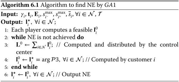
Algorithm 6.1 is proposed to approach the NE of ![]() .
.
Theorem 6.2 demonstrates that ![]() not only favors the customers but also minimizes the total cost and thus favors power suppliers as well. So
not only favors the customers but also minimizes the total cost and thus favors power suppliers as well. So ![]() minimizes PAR according to theorem 6.1. However, the control center may not want to release the price‐calculating function to customers. We then propose another approach based on a precalculated fixed‐price schedule.
minimizes PAR according to theorem 6.1. However, the control center may not want to release the price‐calculating function to customers. We then propose another approach based on a precalculated fixed‐price schedule.
6.4.3 Game Theoretical Approach 2: Semifixed Smart Pricing
In this approach, each customer ![]() also submits an initial load schedule
also submits an initial load schedule ![]() ; however, the price function is hidden from customers. Only the control center is able to calculate the fixed price vector with each
; however, the price function is hidden from customers. Only the control center is able to calculate the fixed price vector with each ![]() as
as
Then each customer ![]() will solve the following problem to find
will solve the following problem to find ![]() ,
,
Note that ![]() is a linear optimization problem, which can be solved with a unique solution. However, the NE for
is a linear optimization problem, which can be solved with a unique solution. However, the NE for ![]() is not guaranteed, since the objective function is no longer strictly concave.
is not guaranteed, since the objective function is no longer strictly concave.
6.4.4 Mixed Approach: Mixed  and
and 
The mixed approach is to apply both ![]() and
and ![]() approaches based on the properties of customers. As mentioned earlier,
approaches based on the properties of customers. As mentioned earlier, ![]() reveals the price function to the customers, which may not favor the control center. The total load is also given to all customers. However, customers who use a significant proportion of energy may not want to reveal such private information.
reveals the price function to the customers, which may not favor the control center. The total load is also given to all customers. However, customers who use a significant proportion of energy may not want to reveal such private information. ![]() does not have those issues but it does not guarantee the optimal solution of
does not have those issues but it does not guarantee the optimal solution of ![]() or
or ![]() . In the mixed approach, large‐energy‐consumption customers adopt
. In the mixed approach, large‐energy‐consumption customers adopt ![]() (e.g. business and industrial customers), and regular‐energy‐consumption customers (e.g. residential customers) adopt
(e.g. business and industrial customers), and regular‐energy‐consumption customers (e.g. residential customers) adopt ![]() . In the numerical analysis and simulation section, we will show that the mixed approach converges to the minimum PAR in practice.
. In the numerical analysis and simulation section, we will show that the mixed approach converges to the minimum PAR in practice.
6.5 Precision and Truthfulness of the Proposed DR System
Because customers could have exceptional energy consumption, a one‐time scheduling approach [28, 29, 99] can hardly be followed strictly. In order to increase the precision of the proposed DR system, the system should run at the beginning of each time interval for the rest of the day. The control center and the computing device of each customer (e.g. the smart meter) should save the previous status and subtract it from the constraints when calculating the load scheduling for the rest of the day. With the DR system following schedule, and since the payment is collected after each time interval based on the real energy usage in that interval, for ![]() ,
, ![]() and
and ![]() , the minimum PAR, the minimum total cost, and the maximum local saving will be achieved only when customers report the load schedules truthfully. The conclusion is quite intuitive because lying about the load will keep customers from reaching the optimal solution. Therefore, the truthfulness of the proposed DR systems should be guaranteed.
, the minimum PAR, the minimum total cost, and the maximum local saving will be achieved only when customers report the load schedules truthfully. The conclusion is quite intuitive because lying about the load will keep customers from reaching the optimal solution. Therefore, the truthfulness of the proposed DR systems should be guaranteed.
6.6 Numerical and Simulation Results
6.6.1 Settings
Assume that power suppliers are available to support customers with any energy requirement. The control center is able to gather information from and distribute it to the power suppliers and the customers in real time (e.g. ![]() ). The customers are categorized into residential, business, and industrial types. Without loss of generality, we assume that the daily energy consumption of the customers follows the proportions obtained from the data in Figure 6.2. Specifically, as shown in Figure 6.4, residential customers consist of three types (i.e. families in big houses, families in townhouses, and families in apartments), each with 55 kilowatt‐hours, 41 kilowatt‐hours, and 33 kilowatt‐hours daily average energy consumption respectively. Each residential customer type has 50 customers. Business customers have two types (i.e. day‐time based business and shopping malls), each with 2400 kilowatt‐hours and 2700 kilowatt‐hours daily average energy consumption respectively, and each type has one customer. Industrial customers have two types (i.e. nonstop shift‐based manufacturers and day‐time based industry), each with 2100 kilowatt‐hours and 2500 kilowatt‐hours daily average energy consumption respectively, and each type has one customer. Note that the settings for the customers are flexible as long as the total energy consumption of each category follows the practical data.
). The customers are categorized into residential, business, and industrial types. Without loss of generality, we assume that the daily energy consumption of the customers follows the proportions obtained from the data in Figure 6.2. Specifically, as shown in Figure 6.4, residential customers consist of three types (i.e. families in big houses, families in townhouses, and families in apartments), each with 55 kilowatt‐hours, 41 kilowatt‐hours, and 33 kilowatt‐hours daily average energy consumption respectively. Each residential customer type has 50 customers. Business customers have two types (i.e. day‐time based business and shopping malls), each with 2400 kilowatt‐hours and 2700 kilowatt‐hours daily average energy consumption respectively, and each type has one customer. Industrial customers have two types (i.e. nonstop shift‐based manufacturers and day‐time based industry), each with 2100 kilowatt‐hours and 2500 kilowatt‐hours daily average energy consumption respectively, and each type has one customer. Note that the settings for the customers are flexible as long as the total energy consumption of each category follows the practical data.

Figure 6.4 Daily consumption of customers.
The granularity of time intervals is important to the DR system. As shown in Figure 6.5 and Figure 6.6, when ![]() , the total load of the power grid is constant throughout the day, while it fluctuates when
, the total load of the power grid is constant throughout the day, while it fluctuates when ![]() .
.

Figure 6.5 Solution to  with
with  .
.

Figure 6.6 Solution to  with
with  .
.
Some of the detailed initial settings for residential customers are shown in Table 6.2. We assume that each storage unit is able to hold ![]() of the daily power usage, each family has 2 PHEVs for type 1 and type 2 residential customers, and customers living in apartments have 1 PHEV each. Each PHEV holds 9 kilowatt‐hours of electricity. The power usage and rough schedules for other appliances are estimates based on day‐to‐day experiences. For simplicity, the on/off schedule is shown as start/end times. Note that some of the appliances are shown as multiple ones to make the modeling more precise; for example, AC for residential users is shown as ventilation all day and fully operating in the afternoon.
of the daily power usage, each family has 2 PHEVs for type 1 and type 2 residential customers, and customers living in apartments have 1 PHEV each. Each PHEV holds 9 kilowatt‐hours of electricity. The power usage and rough schedules for other appliances are estimates based on day‐to‐day experiences. For simplicity, the on/off schedule is shown as start/end times. Note that some of the appliances are shown as multiple ones to make the modeling more precise; for example, AC for residential users is shown as ventilation all day and fully operating in the afternoon.
Table 6.2 Residential settings for the case study.
| App | Start | End | |||
| Residential | |||||
| Storage | 0 | 24 | |||
| PHEV | 0 | 0 | 8 | ||
| AC1 | 0 | 24 | |||
| AC2 | 14 | 18 | |||
| Cooking | 0 | 17,17,18 | 20,20,20 | ||
| Dish washer | 0 | 20,20,20 | 24,23,22 | ||
| Washing/dryer | 0 | 20,20,18 | 24,23,22 | ||
| Electronics | 18 | 24 | |||
| Others | 0 | 24 | |||
6.6.2 Comparison of  ,
,  and
and 
In this subsection, we evaluate the three DR mechanisms, including the two centralized ones and the game theoretical approach where smart pricing is computed locally. Figure 6.7 shows that the ![]() ,
, ![]() , and
, and ![]() all reach the same optimal result with respect to the total load. However, each customer receives a different load scheduling. This is observed in all three DR systems.
all reach the same optimal result with respect to the total load. However, each customer receives a different load scheduling. This is observed in all three DR systems.

Figure 6.7 Load schedules by  ,
,  and
and  .
.
To better illustrate the results from the three DR mechanisms, more detailed results for residential customers are shown in Figure 6.8. Specifically, Figure 6.8(a), Figure 6.8(c), and Figure 6.8(c) show the results for three types of residential customers respectively. For each type of residential customer, the results are given for eight hours only. Note that ![]() leads to a negative load for some customers, as shown in Figure 6.8(c). In the smart grid, some customers sell extra energy from their storage unit when the price is high to maximize their savings.
leads to a negative load for some customers, as shown in Figure 6.8(c). In the smart grid, some customers sell extra energy from their storage unit when the price is high to maximize their savings.
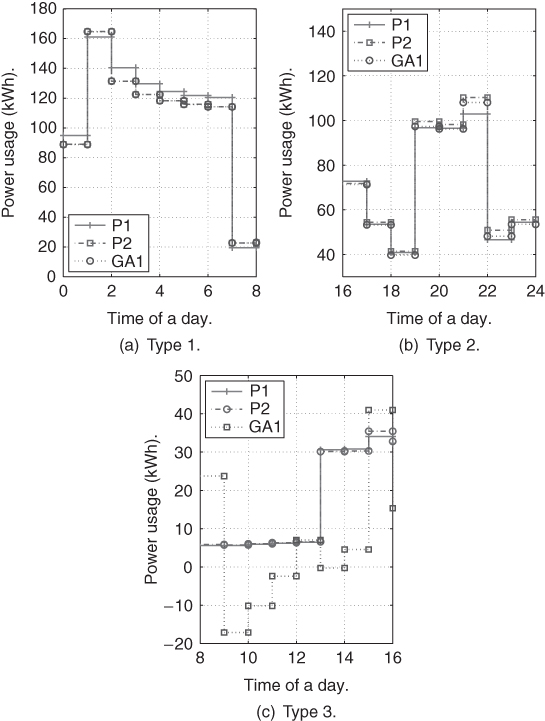
Figure 6.8 Load of different types of residential customers.
Similarly, load schedules for business customers are shown in Figure 6.9. Load schedules for industrial customers are shown in Figure 6.10.
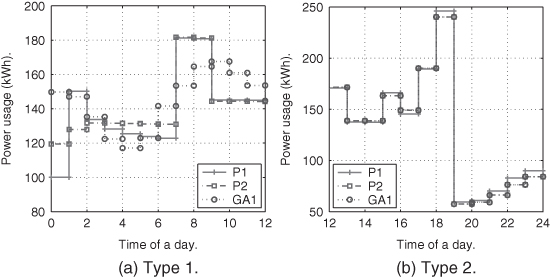
Figure 6.9 Load of different types of business customers.

Figure 6.10 Load of different types of industrial customers.
6.6.3 Comparison of Different Distributed Approaches
Figure 6.11 shows the load scheduling results of ![]() ,
, ![]() , mixed
, mixed ![]() , and a distributed approach when all customers intend to minimize their local PAR. From the simulation results, we can see that both
, and a distributed approach when all customers intend to minimize their local PAR. From the simulation results, we can see that both ![]() and mixed
and mixed ![]() converge to the optimal PAR, while neither
converge to the optimal PAR, while neither ![]() nor min local PAR minimizes PAR.
nor min local PAR minimizes PAR.
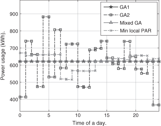
Figure 6.11 Load scheduling from different distributed approaches.
In fact, ![]() performs the worst in the simulation when all customers are considered. Because of the fixed smart price, customers will shift their load to the time intervals with low prices without considering the consequences of doing so. When all customers do so, the time intervals with a relative low previous load will be scheduled with a higher load, and the price will go up. Then customers will shift back based on the updated price schedule. The simulation also indicates that
performs the worst in the simulation when all customers are considered. Because of the fixed smart price, customers will shift their load to the time intervals with low prices without considering the consequences of doing so. When all customers do so, the time intervals with a relative low previous load will be scheduled with a higher load, and the price will go up. Then customers will shift back based on the updated price schedule. The simulation also indicates that ![]() alone fluctuates between these two states without converging to the NE. Figure 6.12 shows the two states of the total load schedule by
alone fluctuates between these two states without converging to the NE. Figure 6.12 shows the two states of the total load schedule by ![]() for the first eight time intervals. Figure 6.13, Figure 6.14, and Figure 6.15 show the average load schedules by
for the first eight time intervals. Figure 6.13, Figure 6.14, and Figure 6.15 show the average load schedules by ![]() and mixed
and mixed ![]() for the first type of customers in each category. It appears that
for the first type of customers in each category. It appears that ![]() schedules a smoother load for each customer, because residential customers have better assessments of the cost changes based on their updated schedule with
schedules a smoother load for each customer, because residential customers have better assessments of the cost changes based on their updated schedule with ![]() . When applying mixed GA, although each customer does not affect the price much, they together still cause a major impact. Therefore, both business and industrial customers must schedule their loads with more fluctuation to adapt to the residential load.
. When applying mixed GA, although each customer does not affect the price much, they together still cause a major impact. Therefore, both business and industrial customers must schedule their loads with more fluctuation to adapt to the residential load.
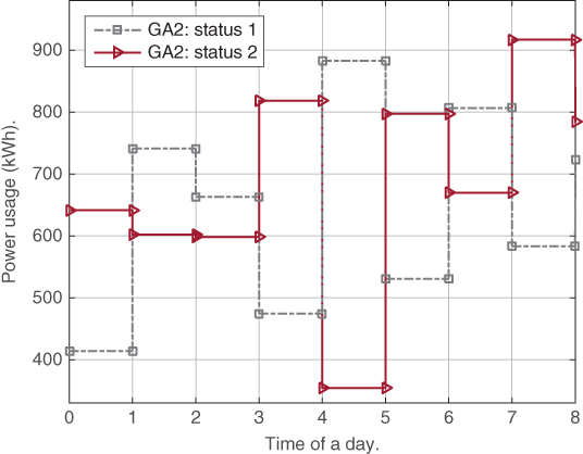
Figure 6.12 illustration.
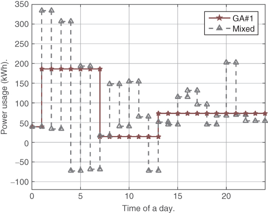
Figure 6.13 Load achieved by  for type
  residential customers.
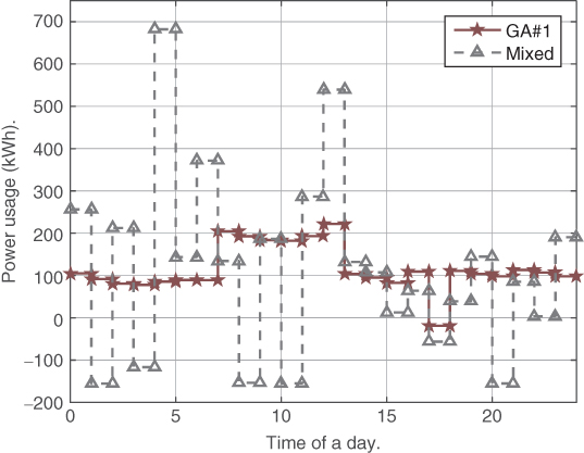
Figure 6.14 Load achieved by  for type
  business customers.

Figure 6.15 Load achieved by  for type
  industrial customers.
Figure 6.16 shows that both ![]() and mixed
and mixed ![]() converge quickly to the NE. In game theoretical approaches, the uplink to the network transmits the load schedule of each customer to the control center, and the control center broadcasts the total load schedule to all customers. Although it requires multiple iterations, it also requires much less data transmission compared with the centralized approach, which needs much more detailed data from the customers, and the scheduled appliance load must be delivered to each customer individually. Moreover, it is worth mentioning that energy providers may not want to declare the true cost function to all the customers in practice. With the adoption of mixed GA, only a few customers are required to know the cost function, and some confidential agreements can be made.
converge quickly to the NE. In game theoretical approaches, the uplink to the network transmits the load schedule of each customer to the control center, and the control center broadcasts the total load schedule to all customers. Although it requires multiple iterations, it also requires much less data transmission compared with the centralized approach, which needs much more detailed data from the customers, and the scheduled appliance load must be delivered to each customer individually. Moreover, it is worth mentioning that energy providers may not want to declare the true cost function to all the customers in practice. With the adoption of mixed GA, only a few customers are required to know the cost function, and some confidential agreements can be made.

Figure 6.16 Convergence of  and mixed
  .
.
6.6.4 The Impact from Energy Storage Unit
Whether to include energy storage units in the smart grid may contribute to DR in the smart grid. From Figure 6.17 we can see that the total load schedule is no longer a straight line without the assistance of storage units. Therefore, storage units on the customers' side will certainly improve the efficiency of DR mechanisms. In theory, if the capacity of the energy storage units is unlimited, the smart grid would have enough buffer to store all electricity that is overgenerated, especially that from renewable power sources. In practice, customer may use electric vehicles as energy storage units in the future.

Figure 6.17 Load schedule without storage units.
Without energy storage units, the PAR for the power grid would be higher, as shown in Figure 6.18. However, storage units may not necessarily help reduce the PAR for each customer individually.

Figure 6.18 Impact of storage units on PAR.
6.6.5 The Impact from Increasing Renewable Energy
In the future, the smart grid will integrate more renewable energy sources. Based on the data shown Figure 6.3, we can estimate the different power suppliers up to the year 2020. As shown in Figure 6.19, renewable energy sources will be more than 20% of the smart grid.
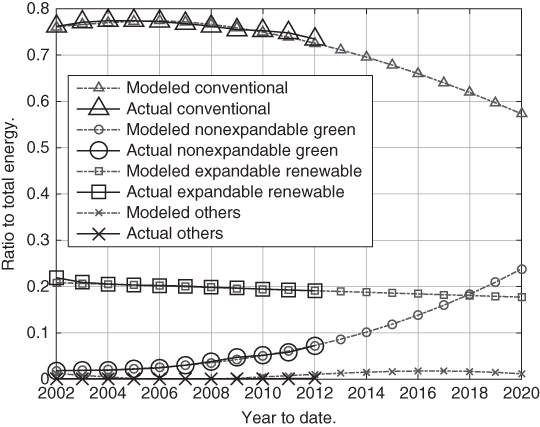
Figure 6.19 An estimate of different power suppliers.
Based on these estimates, the total energy cost to te customers in 2014, 2018, and 2020 is shown in Figure 6.20. Clearly, the expansion of renewable energy would help to reduce energy costs.
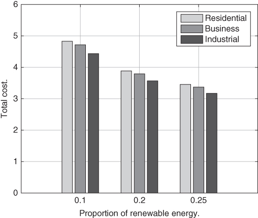
Figure 6.20 Corresponding total cost estimates for future years.
6.7 Summary
In this chapter, we studied demand response in the smart grid. In order to motivate and benefit all parties, including society (the environment), power suppliers, and customers, we proposed several approaches for the DR system. First, ![]() directly minimizes PAR. Second, a DLC‐based cost minimization approach
directly minimizes PAR. Second, a DLC‐based cost minimization approach ![]() motivates the power suppliers. However, both
motivates the power suppliers. However, both ![]() and
and ![]() fail to protect the privacy of customers, and their communication overhead is too high for deployment in a real‐time system. We proposed two further smart pricing‐based game theoretical approaches
fail to protect the privacy of customers, and their communication overhead is too high for deployment in a real‐time system. We proposed two further smart pricing‐based game theoretical approaches ![]() and
and ![]() to address the shortcomings of
to address the shortcomings of ![]() and
and ![]() . We successfully proved that both
. We successfully proved that both ![]() and
and ![]() , in which each customer calculates the dynamic price locally, reach the solution to
, in which each customer calculates the dynamic price locally, reach the solution to ![]() (min PAR). In the numerical analysis and the simulations, we further demonstrated the results and compared the performance of several distributed approaches.
(min PAR). In the numerical analysis and the simulations, we further demonstrated the results and compared the performance of several distributed approaches.