
Chapter 12
General Equilibrium with Heterogeneous Participants and Discrete Consumption Times
Journal of Financial Economics, 108, (2013), pp. 608–614; short version published in FAMe, 2013.
Abstract
The paper investigates the term structure of interest rates imposed by equilibrium in a production economy consisting of participants with heterogeneous preferences. Consumption is restricted to an arbitrary number of discrete times. The paper contains an exact solution to market equilibrium and provides an explicit constructive algorithm for determining the state price density process. The convergence of the algorithm is proven. Interest rates and their behavior are given as a function of economic variables.
Introduction
Interest rates are determined by the equilibrium of supply and demand. Increased demand for credit brings interest rates higher, while an increase in demand for fixed-income investment causes rates to go down. To determine the mechanism by which economic forces and investors' preferences cause changes in supply and demand, it is necessary to develop a general equilibrium model of the economy. Such model provides a means of quantitative analysis of how economic conditions and scenarios affect interest rates.
Vasicek (2005) (Chapter 11 of this volume) investigates an economy in continuous time with production subject to uncertain technological changes described by a state variable. Consumption is assumed to be in continuous time, with each investor maximizing the expected utility from lifetime consumption. The participants have constant relative risk aversion, with different degrees of risk aversion and different time preference functions. After identifying the optimal investment and consumption strategies, the paper derives conditions for equilibrium and provides a description of interest rates.
For a meaningful economic analysis, it is essential that a general equilibrium model allows heterogeneous participants. If all participants have identical preferences, then they will all hold the same portfolio. Since there is no borrowing and lending in the aggregate, there is no net holding of debt securities by any participant, and no investor is exposed to interest rate risk. Moreover, if the utility functions are the same, it does not allow for study of how interest rates depend on differences in investors' preferences.
The main difficulty in developing a general equilibrium model with heterogeneous participants had been the need to carry the individual wealth levels as state variables, because the equilibrium depends on the distribution of wealth across the participants. This can be avoided if the aggregate consumption can be expressed as a function of a Markov process, in which case only this Markov process becomes a state variable. This is often simple in models of pure exchange economies, where the aggregate consumption is exogenously specified.
The situation is different in models of production economies. In such economies, the aggregate consumption depends on the social welfare function weights. Because these weights are determined endogenously, it is necessary that the individual consumption levels themselves be functions of a Markov process. This has precluded an analysis of equilibrium in a production economy with any meaningful number of participants; most explicit results for production economies had previously been limited to models with one or two participants.
The above approach is exploited here. Vasicek (2005) shows that the individual wealth levels can be represented as functions of a single process, which is jointly Markov with the technology state variable. This allows construction of equilibrium models with just two state variables, regardless of the number of participants in the economy.
In Vasicek (2005), the equilibrium conditions are used to derive a nonlinear partial differential equation whose solution determines the term structure of interest rates. While the solution to the equation can be approximated by numerical methods, the nonlinearity of the equation could present some difficulties.
The present paper provides the exact solution for the case that consumption takes place at a finite number of discrete times. This solution does not require solving partial differential equations, and explicit computational procedure is provided. If the time points are chosen to be dense enough, the discrete case will approximate the continuous case with the desired precision. Some may in fact argue that, in reality, consumption is discrete rather than continuous, and therefore the discrete case addressed here is the more relevant.
The following section summarizes the relevant results from Vasicek (2005). The next section contains the solution for the equilibrium state price density process and the structure of interest rates in the discrete consumption case. The final section gives a proof that the proposed algorithm converges to the market equilibrium.
The Equilibrium Economy
Assume that a continuous time economy contains a production process whose rate of return dA/A on investment is
where y(t) is a Wiener process. The process A(t) represents a constant return-to-scale production opportunity. An investment of an amount W in the production at time t yields the amount WA(s)/A(t) at time s > t. The production process can be viewed as an exogenously given asset that is available for investment in any amount. The amount of investment in production, however, is determined endogenously.
The parameters of the production process can themselves be stochastic. It will be assumed that their behavior is driven by a Markov state variable ![]() . The dynamics of the state variable, which can be interpreted as representing the state of the production technology, is given by
. The dynamics of the state variable, which can be interpreted as representing the state of the production technology, is given by
where ![]() is a Wiener process independent of
is a Wiener process independent of ![]() . The parameters
. The parameters ![]() , and ϕ are functions of
, and ϕ are functions of ![]() and t.
and t.
It is assumed that investors can issue and buy any derivatives of any of the assets and securities in the economy. The investors can lend and borrow among themselves, either at a floating short rate or by issuing and buying term bonds. The resultant market is complete. It is further assumed that there are no transaction costs and no taxes or other forms of redistribution of social wealth. The investment wealth and asset values are measured in terms of a medium of exchange that cannot be stored unless invested in the production process. For instance, this wealth unit could be a perishable consumption good.
Suppose that the economy has n participants and let ![]() be the initial wealth of the k–th investor. Each investor maximizes the expected utility from lifetime consumption,
be the initial wealth of the k–th investor. Each investor maximizes the expected utility from lifetime consumption,

where ![]() is the rate of consumption at time
is the rate of consumption at time ![]() is a utility function with
is a utility function with ![]() , and
, and ![]() is a time preference function. Consider specifically the class of isoelastic utility functions, written in the form
is a time preference function. Consider specifically the class of isoelastic utility functions, written in the form

Here ![]() is the reciprocal of the relative risk aversion coefficient,
is the reciprocal of the relative risk aversion coefficient, ![]() , which will be called the risk tolerance.
, which will be called the risk tolerance.
An economy cannot be in equilibrium if arbitrage opportunities exist in the sense that the returns on an asset strictly dominate the returns on another asset. A necessary and sufficient condition for absence of arbitrage is that there exist processes ![]() , called the market prices of risk for the risk sources
, called the market prices of risk for the risk sources ![]() , respectively, such that the price P of any asset in the economy satisfies the equation
, respectively, such that the price P of any asset in the economy satisfies the equation
where ![]() are the exposures of the asset to the two risk sources. In particular,
are the exposures of the asset to the two risk sources. In particular,
It is assumed that Novikov's condition holds,

Let Z be the numeraire portfolio of Long (1990) with the dynamics
such that the price P of any asset satisfies
Specifically, the price ![]() at time t of a default-free bond with unit face value maturing at time s is given by the equation
at time t of a default-free bond with unit face value maturing at time s is given by the equation
Here and throughout, the symbol Et denotes expectation conditional on a filtration ℑt generated by ![]() . In integral form, the numeraire portfolio can be written as
. In integral form, the numeraire portfolio can be written as

The process ![]() is the reciprocal of the state price density process.
is the reciprocal of the state price density process.
Vasicek (2005) shows that the optimal consumption rate of the k-th investor is a function of the numeraire process only, given as
where

is a constant. The individual wealth level Wk under an optimal strategy is

The behavior of the wealth level ![]() is fully determined by the process
is fully determined by the process ![]() . Moreover, the process
. Moreover, the process ![]() is Markov. That means that
is Markov. That means that ![]() is a function of two state variables X and Z only.
is a function of two state variables X and Z only.
In equilibrium, the total wealth
must be invested in the production process (which justifies referring to the production process as the market portfolio). Any lending and borrowing (including lending and borrowing implicit in issuing and buying contingent claims) is among the participants in the economy, and its sum must be zero. Thus, the total exposure to the process y is that of the total wealth invested in the production, and the total exposure to the process x is zero. This produces the equation
describing the dynamics of the total wealth. The terminal condition is
The process Z is further subject to the requirement that
The unique solution of the stochastic differential Eq. (16) subject to Eqs. (17) and (18) is given by

In Vasicek (2005), the process ![]() is determined in the following manner: Write
is determined in the following manner: Write ![]() as a function of the state variables. Expanding dW in Eq. (16) by Ito's lemma and comparing the coefficients of
as a function of the state variables. Expanding dW in Eq. (16) by Ito's lemma and comparing the coefficients of ![]() , and dx provides equations from which λ, η can be eliminated, resulting in a nonlinear partial differential equation with known coefficients. Once the function
, and dx provides equations from which λ, η can be eliminated, resulting in a nonlinear partial differential equation with known coefficients. Once the function ![]() has been determined as the unique solution of this equation, λ and η are calculated from
has been determined as the unique solution of this equation, λ and η are calculated from ![]() as functions of
as functions of ![]() , and t. The process
, and t. The process ![]() is obtained by integrating the stochastic differential equation (8). Bond prices are determined from Eq. (10).
is obtained by integrating the stochastic differential equation (8). Bond prices are determined from Eq. (10).
In the case of discrete consumption dealt with in this paper, the partial differential equation and the subsequent integration of Eq. (8) is replaced by an explicit algorithm described in the next section.
Equilibrium is fully described by specification of the process Z(t), which determines the pricing of all assets in the economy, such as bonds and derivative contracts, by means of Eq. (9). Solving for the equilibrium requires determining the values of the constants ![]() . The algorithm proposed in this paper utilizes the fact that any choice of the constants is consistent with a unique equilibrium described by the process
. The algorithm proposed in this paper utilizes the fact that any choice of the constants is consistent with a unique equilibrium described by the process ![]() , except that the corresponding initial wealth levels calculated as
, except that the corresponding initial wealth levels calculated as

do not agree with the given initial values ![]() . Repeatedly replacing
. Repeatedly replacing ![]() by
by ![]() and recalculating Z converges to the required equilibrium, as proven in “Proof of Convergence” section later in this chapter. This is analogous to the method proposed by Negishi (1960) in a deterministic economy.
and recalculating Z converges to the required equilibrium, as proven in “Proof of Convergence” section later in this chapter. This is analogous to the method proposed by Negishi (1960) in a deterministic economy.
In economic literature, the usual approach to investigating the existence and uniqueness of equilibrium has been the concept of a representative agent (see Negishi, 1960, and Karatzas and Shreve, 1998). The representative agent maximizes an objective (the social welfare function)

where ![]() is the consumption rate of the agent (equal to the aggregate consumption of all participants) and
is the consumption rate of the agent (equal to the aggregate consumption of all participants) and ![]() are weights assigned to the individual participants. The constants
are weights assigned to the individual participants. The constants ![]() in Eq. (12) are related to the representative agent weights. Eq. (4.5.7) in Theorem 4.5.2 of Karatzas and Shreve (1998) can be written as
in Eq. (12) are related to the representative agent weights. Eq. (4.5.7) in Theorem 4.5.2 of Karatzas and Shreve (1998) can be written as
Comparing Eqs. (22) and (12) yields the relationship
for ![]() .
.
Discrete Consumption Times
This chapter considers an economy in which consumption takes place only at specific discrete dates. The economy exists in continuous time, and between the consumption dates the participants are continuously trading and the production is continuous. The market is assumed to be complete.
Suppose each investor's time preference function is concentrated at positive points ![]() , so that the k-th investor maximizes the expected utility
, so that the k-th investor maximizes the expected utility
where ![]() is the consumption at time
is the consumption at time ![]() , and
, and ![]() is a utility function given by Eq. (4). It is assumed that
is a utility function given by Eq. (4). It is assumed that
Let ![]() be the state price density process. Put
be the state price density process. Put
for ![]() , with
, with ![]() . The state variable
. The state variable ![]() can be a vector. Furthermore, let
can be a vector. Furthermore, let
for ![]() , and
, and ![]() .
.
The optimal individual consumption is given from Eq. (12) by
for ![]() , where
, where ![]() are positive constants satisfying the equation
are positive constants satisfying the equation

Eq. (16) takes the form
and
where
From Eq. (31),
From Eq. (18),
Note that Eqs. (33) and (34) imply
as is easily established by multiplying Eq. (33) by ![]() and taking expectation.
and taking expectation.
The solution to Eqs. (31) and (34) subject to ![]() is obtained by successive elimination of
is obtained by successive elimination of ![]() and
and ![]() ,
, ![]() . Let
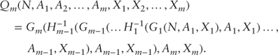
. Let ![]() be the inverse of the function Km and define recursively two sets of functions
be the inverse of the function Km and define recursively two sets of functions ![]() as follows:
as follows:
and ![]() is the positive solution of the equation
is the positive solution of the equation
for ![]() ; and
; and
for ![]() . Then
. Then
It will be now shown that the functions ![]() are decreasing functions of the first argument. Suppose, for some
are decreasing functions of the first argument. Suppose, for some ![]() is a decreasing function of N. It follows from Eq. (38) that
is a decreasing function of N. It follows from Eq. (38) that ![]() is also decreasing in N. Denote by
is also decreasing in N. Denote by ![]() the inverse of the function
the inverse of the function ![]() with respect to the first argument while keeping the remaining arguments constant. Then from Eq. (37),
with respect to the first argument while keeping the remaining arguments constant. Then from Eq. (37),
The expression on the left-hand side of this equation is a decreasing function of Gi–1, and therefore the function ![]() is decreasing in N. Because
is decreasing in N. Because ![]() is decreasing in N, it follows by induction that
is decreasing in N, it follows by induction that ![]() , and consequently
, and consequently ![]() , are all decreasing functions of the first argument.
, are all decreasing functions of the first argument.
Then from Eq. (39),
for ![]() . Eq. (41) together with
. Eq. (41) together with ![]() determines
determines ![]() recursively. The state price density process at time t is
recursively. The state price density process at time t is
Eqs. (41), (42) represent the exact solution to the equilibrium economy in the case that consumption is limited to a number of discrete times, provided Eq. (29) holds.
Calculation of the equilibrium solution proceeds as follows: Choose initial values of the constants ![]() . A reasonable initial guess is
. A reasonable initial guess is

for ![]() . Calculate recursively the functions
. Calculate recursively the functions ![]() and
and ![]() from Eqs. (36), (37), and (38). Calculate
from Eqs. (36), (37), and (38). Calculate ![]() and determine
and determine ![]() from Eq. (41). Calculate
from Eq. (41). Calculate ![]() as
as
for ![]() . Set new values of constants
. Set new values of constants ![]() as
as
Repeat the above calculations with the new values of the constants until ![]() are sufficiently close to
are sufficiently close to ![]() . The state price density process is given by Eq. (42). Bond prices are given as
. The state price density process is given by Eq. (42). Bond prices are given as
Interest rates are determined by bond prices.
In the special case that ![]() , the functions take the form
, the functions take the form ![]() ,
, ![]() ,
, ![]() ,
, ![]() , where
, where ![]() ,
,

and
Then
and

Proof of Convergence
Define the function ![]() as
as
Since there is an odd number of decreasing functions in the nested expression (51), ![]() is a decreasing function of N. Then
is a decreasing function of N. Then
Note that Eq. (52) represents the solution to Eqs. (33) and (34), since the intermediate values of ![]() have been eliminated.
have been eliminated.
Assume that ![]() (corresponding to the sufficient condition (4.6.4) for uniqueness of the equilibrium solution in Theorem 4.6.1 in Karatzas and Shreve, 1998). Let
(corresponding to the sufficient condition (4.6.4) for uniqueness of the equilibrium solution in Theorem 4.6.1 in Karatzas and Shreve, 1998). Let ![]() be arbitrary positive constants and determine
be arbitrary positive constants and determine ![]() from Eq. (39). Calculate
from Eq. (39). Calculate ![]() from Eq. (44) and
from Eq. (44) and ![]() from Eq. (45),
from Eq. (45), ![]() . Put
. Put
and denote by ![]() the variables calculated using the constants
the variables calculated using the constants ![]() in place of
in place of ![]() . Then
. Then
and
Put
and
Define

Then

Set

![]() . Let
. Let ![]() be the lowest and highest value, respectively, of
be the lowest and highest value, respectively, of ![]() , and
, and ![]() be the lowest and highest value, respectively, of
be the lowest and highest value, respectively, of ![]() . Put
. Put
k = 1, 2,…, n. Note that
and therefore
Define
and put
The values ![]() satisfy the relationship
satisfy the relationship
Eqs. (65) and (66) have the solution
Now

for ![]() , and consequently
, and consequently
Because ![]() is a decreasing function of its first argument, Eqs. (52) and (67) imply
is a decreasing function of its first argument, Eqs. (52) and (67) imply
It is proven similarly that
and from Eqs. (34) and (55) it then follows that
for ![]() .
.
From Eq. (59),
and consequently
If ![]() , then
, then
and
If ![]() , then
, then
and
Thus, either the inequality in Eq. (76) or (78) holds.
Put ![]() and let l be such that
and let l be such that ![]() . Then
. Then

and therefore
Similarly, if l is such that ![]() , then
, then

and therefore
Here ![]() are the lowest and highest value, respectively, of
are the lowest and highest value, respectively, of ![]() , and
, and ![]() is the lowest value of
is the lowest value of ![]() . Put
. Put
Combining the inequalities in Eqs. (76), (78), (80), and (82) produces
Now consider the sequence of iterations ![]() and
and ![]() . The series
. The series ![]() ,
, ![]() is nonincreasing due to the inequality (84) and bounded from below by unity, so it converges to a limit
is nonincreasing due to the inequality (84) and bounded from below by unity, so it converges to a limit ![]() . Assume that
. Assume that ![]() . Because
. Because ![]() is a decreasing function of
is a decreasing function of ![]() and the series
and the series ![]() decrease at least as fast as a geometric series with quotient
decrease at least as fast as a geometric series with quotient ![]() . In a finite number of terms, it falls below the level
. In a finite number of terms, it falls below the level ![]() . Therefore, the assumption that
. Therefore, the assumption that ![]() is false, and
is false, and ![]() converges to unity. Then
converges to unity. Then ![]() and therefore
and therefore ![]() converge to unity and from Eq. (58), the sequence of the iterated values
converge to unity and from Eq. (58), the sequence of the iterated values ![]() converges to
converges to ![]() .
.
Concluding Remarks
This paper provides explicit procedure to obtain the exact solution of equilibrium pricing in a production economy with heterogeneous investors. Each investor maximizes the expected utility from lifetime consumption, taking place at discrete times. Interest rates are determined by economic variables such as the characteristics of the production process, the individual investors' preferences, and the wealth distribution across the participants. Such a model provides a tool for quantitative study of the effect of changes in economic conditions on interest rates.
The algorithm is constructive and converges to the equilibrium solution. The convergence is proven for the case of ![]() , for which the uniqueness of the equilibrium has been established (cf. Karatzas and Shreve, 1998). All other steps of the procedure, however, are valid in general for any positive values of the risk tolerance coefficients. If some of the
, for which the uniqueness of the equilibrium has been established (cf. Karatzas and Shreve, 1998). All other steps of the procedure, however, are valid in general for any positive values of the risk tolerance coefficients. If some of the ![]() are smaller than unity and the values
are smaller than unity and the values ![]() fail to converge to the input values
fail to converge to the input values ![]() after a reasonable number of iterations, a search over the space of positive values of
after a reasonable number of iterations, a search over the space of positive values of ![]() needs to be made.
needs to be made.
While this paper concentrates on the case that the participants have isoelastic utility functions (4), it can be extended to more general class of utilities. Suppose the k-th investor maximizes the objective (24), where ![]() has a positive, decreasing continuous derivative
has a positive, decreasing continuous derivative ![]() with
with ![]() ,
, ![]() ,
, ![]() . Denote the inverse of the derivative by
. Denote the inverse of the derivative by ![]() . Then the optimal consumption is given by
. Then the optimal consumption is given by
where ![]() is a positive constant satisfying the condition
is a positive constant satisfying the condition
for ![]() (cf. Karatzas and Shreve, 1998, Theorems 3.6.3 and 4.4.5). Put
(cf. Karatzas and Shreve, 1998, Theorems 3.6.3 and 4.4.5). Put
Then Eqs. (30), (31), and (33) through (42) still hold. The algorithm consisting of making an initial choice of the constants ![]() , determining
, determining ![]() from Eqs. (39) and (31), setting new values of the constants from Eq. (86), and repeating the calculations may still be applicable, although a proof of convergence is not provided here.
from Eqs. (39) and (31), setting new values of the constants from Eq. (86), and repeating the calculations may still be applicable, although a proof of convergence is not provided here.
References
- Karatzas, I., and S. Shreve. (1998). Methods of Mathematical Finance. New York: Springer-Verlag.
- Long, J. (1990). “The Numeraire Portfolio.” Journal of Financial Economics, 26, 29–69.
- Negishi, T. (1960). “Welfare Economics and Existence of an Equilibrium for a Competitive Economy.” Metroeconomica, 12, 92–97.
- Vasicek, O. (2005). “The Economics of Interest Rates.” Journal of Financial Economics, 76, 293–307.