Search in book...
Toggle Font Controls
Create new playlist

Name your new playlist

Playlist description (optional)
Sign In

Email address

Password

Forgot Password?

or

Continue with Facebook

Continue with Google
Sign Up

Full Name

Email address

Confirm Email Address

Password

or

Continue with Facebook

Continue with Google

Chapter 12
Integrated Supply Chain Models

12.1 Introduction

We have discussed various aspects of managing a supply chain, and most of the earlier chapters focus on one important decision in the supply chain while assuming the other decisions have already been made. For example, when we discuss inventory models, we ignore the facility location decision and its associated costs, whereas in the chapters dealing with location models, we ignore the inventory and shortage costs, as well as the demand uncertainty and the effects that reorder policies have on inventory and shipping costs. One reason for this disconnect is that the decision‐maker may not possess detailed information about the future costs and other parameters in the supply chain when making facility location or network design decisions. Another reason is that the more decisions that are included in a single model, the more complex and hard to solve the model becomes. On the other hand, ignoring inventory, transportation, and other costs when making strategic decisions can lead to suboptimality. Significant cost savings can often be attained by optimizing several of the major cost drivers that can influence the performance of the supply chain.

Recall from Chapter 1 that supply chain decisions can be classified into three levels: strategic, tactical, and operational. Often, decisions are made at each level sequentially. For example, we might first optimize facility locations (a strategic decision) with the expectation that the facilities we choose will operate for roughly 10 years. Each month, we might make tactical inventory decisions at the facilities in anticipation of that month's demand. Finally, we might optimize vehicle delivery routes (an operational decision) every day. Under this sequential approach, higher‐level decisions ignore the lower‐level considerations (we ignore inventory when optimizing facility locations, and we ignore routing when optimizing inventory), whereas the lower level takes the higher‐level decisions as inputs (inventory models assume facility locations are fixed, and routing models assume inventory policies are fixed). In this chapter, we explore models that make decisions at multiple levels simultaneously.

When one considers whether to include decisions at multiple levels in the same optimization model, it is important to ask whether the decisions in the lower‐level problems would affect the decisions at the higher level. For example, in Section 12.2, we consider a model that considers inventory costs when making facility location decisions. We will show that this model chooses different facility locations than we would obtain if we ignored inventory when locating facilities, and moreover, that the location‐only solution is more expensive than the joint solution when inventory costs are factored in. This justifies the increased complexity of a joint location–inventory model and the computational burden required to solve it. On the other hand, suppose we were considering developing a model that chooses the locations of facilities simultaneously with the number of restrooms in each facility. It is unlikely that the locations chosen would be significantly different if each facility has 2 restrooms than they would if each facility has 12 restrooms. In this case, it is probably simpler—from both a modeling and a computational perspective—to optimize the facility locations first, and then optimize the number of restrooms in a separate model.

In this chapter, we discuss three types of integrated models: location–inventory, location–routing, and inventory–routing. We cover a location–inventory model thoroughly in Section 12.2, including details on mathematical formulations, solution approaches, and analytical properties. We then discuss some basic formulations and possible variations of location–routing and inventory–routing problems in Sections 12.3 and 12.4, respectively. We refer interested readers to more comprehensive surveys (e.g., Nagy and Salhi (2007), Shen (2007), Coelho et al. (2013), and Prodhon and Prins (2014)) for more details.

12.2 A Location–Inventory Model

12.2.1 Introduction

We consider the design of a three‐echelon supply chain consisting of one or more suppliers, distribution centers (DCs), and retailers. Each retailer places random demands to the DC that supplies it. The problem is to determine how many DCs to locate, where to locate them, which retailers to assign to each DC, how often to reorder at the DC, and what level of safety stock to maintain, so as to minimize total location, shipment, and inventory costs, while ensuring a specified level of service.

We assume that location costs are incurred when DCs are established. Line‐haul transportation costs are incurred for shipments from a supplier to the DCs. Local transportation costs are incurred in moving the goods from the DCs to the retailers. Inventory costs are incurred at each DC and consist of the holding cost for the average inventory used over a period of time as well as safety stock inventory carried to protect against stockouts that might result from uncertain retailer demand. We assume that the retailers maintain only a minimal amount of inventory, which is ignored in the model below.

In an inventory system, both the cycle stock and the safety stock tend to be concave functions of the demand served. To take a simple example, suppose the demand is distributed as $images$ for $images$ . As we increase $images$ , we scale both the mean and variance. If the cycle stock is set using the economic order quantity (EOQ) formula (we will see below why this is a reasonable assumption), then

(12.1)

And, again for reasons to be discussed below, the safety stock is given by

(12.2)

where $images$ is the desired service level. The right‐hand sides of both 12.1 and 12.2 are concave functions of $images$ .

The upshot of this analysis is that, given the choice between many small facilities or few large facilities to serve a geographically dispersed demand, inventory costs would always favor the latter—both because of the economies of scale present in cycle stock costs and because of the risk‐pooling effect with regard to safety stock costs (see Section 7.2). Of course, this doesn't mean we should always locate only a single DC. Rather, we must consider the fixed costs of the DCs and their locations (and hence transportation costs) before deciding how many DCs to open, and where. The location model with risk pooling (LMRP), ¹ introduced by Daskin et al. (2002) and Shen et al. (2003), simultaneously optimizes all of these factors.

As we will see below, the LMRP is structured much like the uncapacitated fixed‐charge location problem (UFLP), with two extra nonlinear terms in the objective function that represent the cycle‐ and safety‐stock costs. Importantly, these costs are calculated without including any decision variables to represent inventory decisions. Despite its nonlinear (in fact, concave) objective function, the LMRP can be solved quite efficiently using extensions of algorithms for the UFLP.

Imagine a set of retailers, each with random demand. Some of these retailers will be converted to DCs, which will then serve the non‐DC retailers (as well as their own demand). The discussion of the UFLP in Section 8.2 referred to “customers” instead of “retailers,” but the terms are interchangeable—both refer to some source of demand. Also, by stating that some retailers will be “converted” into DCs, we are assuming that $images$ (using the notation of Section 8.2.2). We can make this assumption without loss of generality since if there is a retailer that is not a potential facility site, we can set its fixed cost to $images$ , while if there is a potential facility site that is not a retailer, we can set its demand to 0.

The original motivation for the LMRP was a study of a Chicago‐area blood bank system, in which inventories of blood platelets (an expensive and perishable component of donated blood) were being stored at individual hospitals, which ordered them from the blood bank's main headquarters. The hospitals were doing a poor job of managing these inventories: Some hospitals were routinely throwing away expired platelets because they had ordered too much, while others were chronically understocked and were requesting expensive emergency shipments from the blood bank. The hope was that certain hospitals could be established as distribution centers that would serve their own demand as well as those of nearby hospitals. This would allow the total amount of inventory to remain low while meeting the same service level requirements, due to the risk pooling effect. Moreover, the cost of shipments (both regular and emergency) would decrease since hospitals would now be located closer to their suppliers (Daskin et al., 2002).

The LMRP is not the only location–inventory model in the literature. For example, Barahona and Jensen (1998) consider a fixed cost to stock a given product at each DC; they solve their model using column generation. Their model is tractable but does not capture the costs of cycle and safety stock as accurately as the LMRP. Erlebacher and Meller (2000) formulate a much richer model, but it is highly nonlinear and they propose heuristics to solve it. Teo et al. (2001) consider a model that is similar to the LMRP but without transportation costs; they propose a $images$ ‐approximation algorithm for it. Nozick and Turnquist (2001a,b) linearize the inventory costs in their location–inventory models, and therefore do not capture economies of scale or risk pooling. Teo and Shu (2004) propose a location–inventory model that is similar to the LMRP except that demands are deterministic and the inventory costs are calculated using a power‐of‐two approximation developed by Roundy (1985). Naseraldin and Herer (2008) use a continuous approximation in which customers are located along a line segment and facilities have newsvendor‐type costs; they solve their model analytically to determine the optimal number and locations of facilities on the line segment.

12.2.2 Problem Statement

Let I be the set of retailers, each of which faces normally distributed daily demands. Demands are assumed to be independent both among retailers and from day to day. The objective of the LMRP is to determine how many DCs to locate, where to locate them, and which retailers to assign to each DC to minimize the total expected location, per‐unit, and inventory costs, while ensuring a specified level of service. Each DC receives product from a single supplier. Each DC is assumed to follow an $images$ policy to maintain its inventory, with a type‐1 service level requirement. The cost of such a policy is calculated in the LMRP using the method described in Section 5.3.1.3: Q is set using the deterministic EOQ formula, and r is set using (5.21).

12.2.3 Notation

Define the following notation:

Set
I	= set of retailers/potential DC sites
Parameters
Demand
$images$	= mean daily demand of retailer i
$images$	= variance of daily demand at retailer i
Costs
$images$	= fixed (daily) cost to open a DC at site j
$images$	= fixed cost for DC j to place an order from the supplier, including fixed
	components of both ordering and transportation costs
$images$	= per‐unit cost for each item ordered by DC j from the supplier,
	including per‐unit inbound transportation costs
$images$	= per‐unit outbound transportation cost from DC j to retailer i
$images$	= holding cost per unit per day at DC j
Other
$images$	= lead time (in days) for orders placed by DC j to the supplier
$images$	= desired fraction of DC order cycles during which no stockout occurs
Decision Variables
$images$	= 1 if retailer j is selected as a DC, 0 otherwise
$images$	= 1 if retailer i is served by DC j, 0 otherwise

12.2.4 Objective Function

The objective function will be of the form

Location Cost: The fixed location cost is given by

(12.3)

Per‐Unit Costs: The per‐unit costs have two parts: the inbound cost (which includes both purchase and transportation costs from the supplier), given by

(12.4)

and the outbound cost, given by

(12.5)

Inventory Costs: Consider a single DC j. We know from (5.22) that, under the expected‐inventory‐level (EIL) approximation, the optimal expected cost of an $images$ inventory policy with a type‐1 service level constraint at DC j is given by

where $images$ and $images$ are the mean and standard deviation of the daily demand served by j. However, $images$ and $images$ are not known in advance; they depend on the decision variables. In particular:

Therefore, the expected inventory cost at DC j is given by

(12.6)

The first term in 12.6 is the cycle stock cost, while the second is the safety stock cost. Put another way, the first term represents the economies of scale from consolidating DCs (and therefore orders), while the second represents the risk‐pooling effect: As more demand is added to DC j, the amount of safety stock increases as the square root of the demand served. For both terms, adding a new retailer's demand to DC j moves the cost along the flatter part of the square‐root curve, while establishing the retailer as its own DC starts it all over again at the steeper part.

Note that this concise formulation for the inventory cost would not be possible if we didn't have a closed‐form expression for the optimal EOQ cost, as in (3.5), or safety stock cost, which derives from (4.24). If, to calculate the optimal EOQ cost, it was necessary to run an algorithm to find $images$ and then to plug $images$ into the cost function, then we'd need to include a variable for $images$ and somehow optimize these when we optimize all the other decision variables. This would complicate the model and algorithm considerably.

Combining 12.3–12.6, we get the following objective function:

(12.7)

12.2.5 NLIP Formulation

The LMRP can now be formulated as a nonlinear integer program (NLIP):

(12.8)

(12.9)

(12.10)

(12.11)

(12.12)

Constraints 12.10 require each retailer to be assigned to some DC, and constraints 12.11 require that DC to be open. Constraints 12.11 and 12.12 are integrality constraints. Notice that the LMRP has the exact same constraints as the UFLP—only the objective function is different. (Actually, in the UFLP, constraints (8.7) are nonnegativity constraints, not integrality constraints. But as we said in Section 8.2.2, the nonnegativity constraints in the UFLP can be replaced with integrality constraints without changing the problem.) This suggests that the Lagrangian relaxation method described in Section 8.2.3 might be adapted to solve the LMRP. That is exactly the approach that Daskin et al. (2002) take, and the approach we discuss in Section 12.2.6. We discuss two more approaches to solving the LMRP—one based on column generation and one based on conic optimization—in Sections 12.2.7 and 12.2.8, respectively. Our aim is to demonstrate that many of the fundamental tools of optimization can be brought to bear on complex supply chain optimization problems such as the LMRP.

12.2.6 Lagrangian Relaxation

As in the UFLP, we will solve the LMRP by relaxing the assignment constraints 12.10 to obtain the following Lagrangian subproblem:

12.13

(12.14)

(12.15)

(12.16)

12.2.6.1 Solving the Subproblem

Just like the subproblem for the UFLP, we can decompose $images$ by j. Unfortunately, computing the benefit $images$ is not as straightforward as it was for the UFLP because of the square‐root terms. Instead, for each j, we need to solve the following problem:

(12.17)

(12.18)

Although $images$ is a concave integer minimization problem, it can be solved relatively efficiently—in order $images$ time, using an algorithm developed by Shu et al. (2005). We won't discuss this algorithm. Instead, we'll discuss an even more efficient algorithm that relies on the following assumption:

At first glance, this seems like an unreasonable assumption to make. However, if the demands come from a Poisson process (as is commonly assumed), Assumption 12.1 holds exactly, since the variance of the Poisson distribution equals its mean (hence $images$ for all i). Now 12.17 can be rewritten as follows:

We have gotten rid of one of the square‐root terms, which allows us to rewrite $images$ as:

(12.19)

(12.20)

where

It turns out that $images$ can be solved even more efficiently than $images$ , in $images$ time. We will describe the algorithm shortly. First, let $images$ ; that is, $images$ is the set of retailers that have negative $images$ . Let $images$ and $images$ . Note that $images$ since $images$ for all i. We will further assume that the elements of $images$ are indexed and sorted such that

where $images$ . The algorithm for solving $images$ relies on the following theorem:

Proof

(1) follows from the fact that for all i, $images$ ; if $images$ as well, then the objective function does not increase when $images$ as opposed to $images$ . (2) follows from the fact that if $images$ and $images$ , then setting $images$ decreases the objective function.

To prove (3), suppose, for a contradiction, that $images$ is an optimal solution such that $images$ for some $images$ but $images$ for some $images$ . Define two new solutions $images$ and $images$ as follows:

In other words, $images$ except that $images$ is changed to 1, and $images$ except that $images$ is changed to 0. (See Figure 12.1.) Let $images$ , $images$ , and $images$ be the objective values of $images$ , $images$ , and $images$ , respectively.

Let $images$ (see Figure 12.1), and let

Then

and

Next, note that

(12.21)

by assumption and that

(12.22)

by the strict concavity of the square‐root function. Therefore,

Since $images$ , we have that $images$ . In other words, $images$ is a strictly better solution than $images$ , violating the assumption that $images$ is optimal. Therefore, $images$ satisfies (3). ▪

Schematic illustration of Proof of Theorem 12.1(c). Filled circles represent yi is equal to 1; open circles represent yi is equal to 0. — Figure 12.1 Proof of Theorem 12.1(c). Filled circles represent $images$ ; open circles represent $images$ .

The upshot of Theorem 12.1 is that an optimal solution to $images$ exists that has the form shown in Figure 12.2. $images$ can therefore be solved using Algorithm 12.1. Note that, in line 5 of the algorithm, we take the sums to equal 0 if $images$ . The step with the most iterations is the sorting step in line 3, which can be performed in $images$ time. The algorithm, therefore, can be performed in $images$ time for each j. At each iteration of the Lagrangian procedure, we must solve $images$ for each j, so the total effort required at each iteration is $images$ . To solve $images$ , we set $images$ if $images$ and set $images$ if $images$ and if $images$ in the optimal solution to $images$ .

Schematic illustration of solution to problem (Pj). Filled circles represent yi is equal to 1; open circles represent yi is equal to 0. — Figure 12.2 Solution to problem $images$ . Filled circles represent $images$ ; open circles represent $images$ .

The proof of Theorem 12.1 did not use any special properties of the square‐root function except its concavity. Therefore, Theorem 12.1 still holds if we replace the square‐root term in 12.19 with any concave function of the total mean demand served by DC j. (Note that this square‐root term is a concave function not only of $images$ , but also of $images$ , the total mean demand served by DC j, since $images$ equals $images$ times a constant that is independent of i.) This means that the Lagrangian relaxation algorithm discussed here can be used to solve (LMRP) if the sum of the square‐root terms in the objective function is replaced by any concave function of the total mean demand served by DC j. This property has allowed the LMRP to be extended in a number of ways; see, e.g., Qi et al. (2010).

12.2.6.2 Finding Upper Bounds

As in the Lagrangian relaxation algorithm for the UFLP, at each iteration we want to convert a solution to the Lagrangian subproblem into a feasible solution for the original problem. As before, we start by opening the facilities that are open in the optimal solution to $images$ . Unlike in the UFLP, however, retailers are not always assigned to their nearest open facilities in the LMRP since assignment costs are based on inventory as well as transportation. In other words, the savings from the risk‐pooling effect and economies of scale may outweigh the increased transportation cost if a retailer is assigned to a more distant facility. (See Problem 12.5.) In fact, it is possible for the following strange thing to happen in an optimal solution to the LMRP: A DC is opened in, say, Chicago, but the retailer in Chicago is served by a DC in Minneapolis instead of the DC in Chicago. This would probably never happen in practice, though, so it's a little inconvenient that our model would allow this to be optimal. Fortunately, if Assumption 12.1 holds, it can be shown that this situation is never optimal.

Once we choose which DCs to open, we assign retailers to DCs as follows. First, we loop through all retailers with $images$ in the optimal solution to $images$ (retailers that are assigned to at least one facility) and assign each retailer to the facility j with $images$ that minimizes the increase in cost based on the assignments already made. Next, we loop through all retailers with $images$ and assign these retailers to the open facility that minimizes the increase in cost based on the assignments already made. Note that we only allow retailers with $images$ to be assigned to DCs for which $images$ , while we allow retailers with $images$ to be assigned to any open DC.

After assigning retailers to DCs in this manner, we may want to apply two improvement heuristics:

Retailer reassignment: For each retailer i, determine whether there is a DC that i can be assigned to instead of its current DC that would decrease the objective value. If so, reassign the retailer. If the reassignment means that the old DC no longer has any retailers assigned to it, it can be closed, saving the fixed cost, as well.
DC exchange: Loop through the DCs, looking for an open DC j and a closed DC k such that if j were closed and k were opened (and retailers reassigned as needed), the objective value would decrease. If such a pair can be found, the DCs are exchanged and the heuristic continues.

12.2.6.3 Other Aspects of the Algorithm

The remaining aspects of the Lagrangian relaxation algorithm (subgradient optimization, branch‐and‐bound) are identical to the algorithm described for the UFLP in Section 8.2.3.

Example 12.1

Return to the 88‐node UFLP instance discussed in Example 8.1. Set the demand means $images$ equal to the demands from Example 8.1 and the variances equal to the means (that is, $images$ ). Let $images$ , $images$ , and $images$ for all $images$ . (Given the magnitude of the demands and costs in Example 8.1—i.e., demands in the hundreds and transportation costs in the $100s or $1000s per unit—it makes sense to assume the product units are large, like cases, and the time unit is 1 month. The parameters given above are consistent with that interpretation.) We'll set $images$ for all j for similar reasons as we did for the EOQ in Section 3.2.2—if the purchase cost is the same at all facilities, it does not affect the optimization, but it does inflate the objective function and water down the difference between the LMRP and the UFLP. Let $images$ , so $images$ . (The full data set is available in the file 88node‐lmrp.xlsx on the book's companion web site.)

The optimal solution for the LMRP for this instance is shown in Figure 12.3. The solution opens four DCs—one fewer than the optimal UFLP solution in Example 8.1—located in Philadelphia, PA; Detroit, MI; Fort Worth, TX; and Fresno, CA. The solution has a total expected monthly cost of $1,057,006. This cost is broken down by type in the first two columns of Table 12.1.

Figure 12.3 Optimal solution to 88‐node LMRP instance. Total cost = $1,057,006.

Table 12.1 Costs for optimal and UFLP‐based solution to 88‐node LMRP instance.

Cost Type	Optimal LMRP Solution ($)	UFLP Solution ($)	% Difference
Fixed	215,200	262,100	21.8
Transportation	573,275	542,538	$images$
Cycle stock	200,475	217,806	8.7
Safety stock	68,056	73,940	8.7
Total	1,057,006	1,096,383	3.7

12.2.6.4 Computational Results

Most papers that introduce Lagrangian relaxation algorithms test the algorithm on one or more data sets. These data sets may come from real‐life problems, but more commonly, they are randomly generated since real‐life data are hard to come by. There are several performance measures of interest when evaluating a Lagrangian relaxation algorithm. For example:

How quickly does the algorithm solve the test problems? CPU times of under a minute are generally considered to be quite fast, but times of an hour or longer can be acceptable as well, depending on the context. Some people argue that for strategic problems like facility location, which might be solved only once every few years, it's acceptable for the algorithm to take several hours. Others argue that these models are typically run many times during the process of fine‐tuning the data and running what‐if scenarios, in which case long run times may be unacceptable.
How large are the test problems? CPU times will be dependent on the size of the test data sets, so they should be evaluated with this in mind. Ideally, the data sets tested should include a range of sizes (in this case, number of retailers) so that the reader gets a sense of how fast the CPU time grows with the problem size and how large a problem the algorithm can handle before it gets too slow.
How tight are the bounds achieved by the Lagrangian process, before branch‐and‐bound begins (i.e., at the root node of the branch‐and‐bound tree)? Just like in the standard LP‐based branch‐and‐bound algorithm, it is important to have tight bounds at the root node, otherwise too much branching may be required before the optimality gap is closed.
How many branch‐and‐bound nodes are required before the optimal solution is found (and proven optimal)? This goes hand‐in‐hand with the previous question, since large root‐node gaps will probably mean that many branch‐and‐bound nodes are required. Note that the optimal solution may be found quite early, but many branch‐and‐bound nodes may be required to prove optimality. That is, if the root‐node gap is large, it's possible that we've already found the optimal solution but that branch‐and‐bound will be required to prove that it is optimal.

The algorithm discussed in this section turns out to be quite efficient by these measures. Daskin et al. (2002) report that they solved problems with up to 150 nodes in under 20 seconds on a desktop computer, with no more than 3 branch‐and‐bound nodes required for each problem. Root‐node gaps are generally less than 1%.

The authors report the following managerial insights. First, the optimal number of DCs increases as the transportation cost increases, and it decreases as the holding cost increases. (This result is not surprising, but it is important for validating the model.) Second, although the optimal solution may involve a few retailers that are assigned to facilities other than the closest (see page 34), forcing retailers to be assigned to their closest facilities (for reasons of convenience) does not generally increase the cost by too much. Finally, fewer DCs are located when inventory is taken into account. That is, a firm that solves the UFLP instead of the LMRP, ignoring inventory, will build too many DCs, because it ignores the tendency toward consolidation brought about by the economies of scale in inventory costs.

Example 12.2

Suppose we solve the 88‐node LMRP example described in Example 12.1 as a UFLP—that is, ignoring the inventory costs. From Example 8.1, we know that the optimal UFLP solution to this instance has five DCs. Assigning retailers as described in Section 12.2.6.2 and applying the LMRP cost function 12.7, we get a total cost of $1,096,383—3.7% greater than the optimal LMRP cost (Figure 12.4). See Table 12.1 for a breakdown of this cost by type. The UFLP‐based solution has greater fixed costs (since it opens more DCs) and smaller transportation costs (since the DCs are closer, on average, to the retailers). It also has greater cycle and safety stock costs, since it uses more inventory locations. This confirms that ignoring inventory when making facility location decisions can be costly, since the resulting solution fails to achieve the economies of scale and risk pooling that a more consolidated solution could achieve.

The UFLP‐based solution includes eight retailers that are assigned to DCs that are not their closest open DC. One example is Minneapolis, MN, which is 213.9 miles from the DC in Topeka, KS, but is instead assigned to the DC in Detroit, MI, which is 268.4 miles away. Why? Suppose we assigned Minneapolis to Topeka, instead. Doing so would save $0.50 ċ (268.4‐213.9)ċ 36.8 = $1002.8 in transportation costs (since $images$ for this retailer and $images$ equals half the distance between i and j). On the other hand, excluding the Minneapolis demand, the Detroit DC has 949.1 units of demand assigned, and the Topeka DC has 242.3. Reassigning Minneapolis from Detroit to Topeka would cost an extra

in cycle stock costs and an extra

in safety stock costs. Therefore, the extra inventory costs more than offset the savings in transportation costs.

The push for consolidation can even be strong enough to abandon some of the DCs altogether. For example, if $images$ instead of $images$ , the UFLP‐based solution consolidates all of the demand into four of the five open DCs, leaving the Topeka DC unused even though its fixed cost is already accounted for.

Figure 12.4 UFLP‐based solution to 88‐node LMRP instance. Total cost = $1,096,383.

In the next two sections, we discuss two additional methods for solving the LMRP, using column generation and conic optimization.

12.2.7 Column Generation

Shen et al. (2003) present a different algorithm for solving the LMRP. Their method involves formulating the problem as a set covering problem and solving it using column generation. Here's an overview of how it works. We also refer interested readers to a brief tutorial on the technique of column generation in Appendix D.2.

First suppose that we could write down every possible subset $images$ . (There are $images$ such subsets.) Let $images$ be the collection of all of these subsets. For each subset $images$ and for each facility $images$ , let $images$ be the cost of serving all of the retailers in R from a DC located at j:

Then choose the cheapest facility in R and call its cost $images$ :

(Note that $images$ is different from $images$ : $images$ is the minimum cost of serving all retailers in R, whereas $images$ is simply the per‐unit ordering cost at DC j.) The idea behind modeling this problem as a set covering problem is to choose several sets from $images$ so that every retailer is contained in exactly one set. Each set corresponds to a group of retailers that will be served by a single facility; $images$ represents the cost of this group.

The set covering model has a single decision variable for each $images$ :

$images$ = 1 if set R is in the solution, 0 otherwise

The set covering formulation of the LMRP is as follows:

(12.24)

(12.25)

(12.26)

The objective function 12.24 computes the cost of all of the sets chosen. Constraints 12.25 say that every retailer must be included in at least one chosen set—that is, every retailer must be assigned to some open facility. Although 12.25 is written with a $images$ , any optimal solution will have each retailer assigned to exactly one facility (why?), so the constraints could be written with an $images$ . This is called a “set covering” problem because the idea is to choose a number of sets to “cover” every element in I.

It seems we have lost two aspects of the original problem in formulating it as a set covering problem. First, (LMRP‐SC) is linear, while (LMRP) is nonlinear. What happened to the nonlinearity? Computing each cost $images$ requires solving a nonlinear problem, so the nonlinearity in (LMRP) is present in the setup to (LMRP‐SC), not in (LMRP‐SC) itself. Second, nothing in the formulation of (LMRP‐SC) indicates which j are chosen—only which sets are chosen. That is, if $images$ and $images$ , we know that retailers 2, 4, 7, and 11 are served by the same DC, and that that DC is either 2, 4, 7, or 11, but which one is it? The answer to this question, too, is hidden in the computation of $images$ . To compute $images$ , we had to compute $images$ for $images$ ; whichever was smallest became $images$ . Somewhere we would have recorded which j gave the best cost, and we'd use that to convert a solution to (LMRP‐SC) into a solution to the original problem.

In principle, we could solve the LMRP by enumerating all the sets in $images$ and then solving (LMRP‐SC). Unfortunately, there are two problems with this approach. First, there are $images$ elements in $images$ —far too many to enumerate. Second, even if we could enumerate $images$ , it's not clear how we would solve (LMRP‐SC). The solution to the first problem is to enumerate a small handful of elements of $images$ first, then identify new elements as needed as the algorithm proceeds. (How do we do this? We'll find out below.) The solution to the second problem is to solve the LP relaxation of (LMRP‐SC), then use branch‐and‐bound if the resulting solution is not integer. It turns out that the set covering problem usually has a very tight LP bound. Sometimes the solution to the LP relaxation is naturally all‐integer; if not, it doesn't usually take much branching to find an optimal integer solution. So in what follows, we'll focus on solving the LP relaxation of (LMRP‐SC), not (LMRP‐SC) itself.

Suppose we have enumerated a subset of $images$ —call it $images$ . We might do this by generating random sets, or using some heuristic. We need to solve the LP relaxation of (LMRP‐SC) including only the sets in $images$ , not all of $images$ . This problem is called the restricted master problem; we will denote it by $images$ :

(12.27)

(12.28)

(12.29)

Now suppose we solve $images$ . Let $images$ ( $images$ ) be an optimal solution. Recall from basic LP theory that any optimal solution to an LP has a corresponding optimal dual solution. Let $images$ ( $images$ ) be the optimal dual solution corresponding to $images$ . Recall also that a solution to a minimization LP is optimal if every variable has nonnegative reduced cost with respect to the dual variables. Therefore, if we were to solve $images$ with all of $images$ instead of just $images$ , $images$ would still be optimal provided that

(12.30)

for each $images$ . So even if we didn't solve $images$ over all of $images$ , we can check whether a given solution is optimal by checking 12.30 for all $images$ . Of course, we don't want to check 12.30 for all $images$ since we can't enumerate $images$ . Instead, we search for an $images$ that violates 12.30. But how?

Let $images$ be the set in $images$ that uses j as its designated DC and has the minimum reduced cost. If $images$ has nonnegative reduced cost for all $images$ , then every $images$ has nonnegative reduced cost. For each j, we can find $images$ by solving the following pricing problem:

(12.31)

(12.32)

A solution to this problem can be converted to a set $images$ by setting

this set has cost

Does this problem look familiar? Of course it does—this is the same problem as $images$ (see page 19), plus a constant ( $images$ ) and with $images$ replaced by $images$ . We already know how to solve this problem.

So, at each iteration of the algorithm, we solve $images$ , then solve the pricing problem above for each j. If the objective function is nonnegative for every j, we have found the optimal solution to $images$ . If it is negative for some j, then we add the corresponding set $images$ to $images$ and solve $images$ again. This method is called column generation since it consists of generating good variables (columns) on the fly.

12.2.8 Conic Optimization

We now introduce a more general approach to solve the LMRP. The approach is based on recent developments in conic integer programming. The basic idea is to reformulate the LMRP as a conic quadratic mixed‐integer program (CQMIP), which can then be solved directly using standard optimization software packages such as CPLEX or Mosek, without the need for specially designed algorithms, such as the column generation algorithm in Section 12.2.7 and the Lagrangian relaxation algorithm in Section 12.2.6. Moreover, it does not require us to make Assumption 12.1 about the variance‐to‐mean ratio at the retailers. The approach we discuss was introduced by Atamturk et al. (2012). Classical facility location problems have also been formulated and solved as conic quadratic programs (see, e.g., Kuo and Mittelmann (2004)).

Let $images$ be auxiliary decision variables that represent the nonlinear terms in the objective function 12.8:

(12.33)

(12.34)

Then the LMRP can be reformulated as an equivalent CQMIP as follows:

(12.35)

(12.36)

(12.37)

(12.38)

(12.39)

The objective function is identical to 12.8 except that the nonlinear terms have been replaced by $images$ and $images$ . Constraints 12.37 and 12.38 enforce the definitions of these two variables, as given in 12.33–12.34. Note that, since $images$ , we have $images$ . Moreover, since $images$ and $images$ have positive coefficients in the objective function, it is sufficient to use inequalities in 12.37–12.38 in place of the equalities in 12.33–12.34.

The objective function of (LMRP‐CQMIP) is linear, and the constraints are all either conic quadratic or linear, so (LMRP‐CQMIP) fits the general form of a CQMIP model and can therefore be solved using a general‐purpose CQMIP solver. Atamturk et al. (2012) report that the computational performance of this method is similar to or better than the Lagrangian relaxation and column generation methods discussed above.

Moreover, this approach is very flexible and can be adapted to handle other extensions of the LMRP. For example, Ozsen et al. (2008) incorporate capacity constraints into the LMRP. This is not as straightforward as it is in the capacitated fixed‐charge location problem (Section 8.3.1) because the capacity applies to the maximum inventory level (the inventory level that occurs immediately after an order arrives) rather than simply to the total annual throughput, as in the CFLP. Moreover, because there is no closed‐form expression for the optimal expected cost of a capacitated $images$ policy (as there is for an uncapacitated policy), the capacitated LMRP model requires an explicit $images$ variable to represent the order‐quantity decision. The expected cycle‐stock cost is expressed in the objective function as

(12.39)

(analogous to the EOQ cost function (3.3)), where $images$ is a decision variable. The safety‐stock cost is still given by the second term in 12.6. As a result, the capacitated LMRP model, as formulated by Ozsen et al. (2008), is neither convex nor concave. Ozsen et al. (2008) propose a heuristic method based on Lagrangian relaxation to solve it. However, Atamturk et al. (2012) show that the capacitated LMRP can be reformulated as a CQMIP, using similar ideas as those given above, and solved using a general‐purpose solver. They also use this approach to solve other variants of the LMRP, such as problems with correlated retailer demands, stochastic lead times, and multiple commodities.

12.3 A Location–Routing Model

Location and routing decisions are closely related, since they both depend on the spatial relationships among the facilities and customers. There is often a cost savings that can be attained when the two decisions are optimized simultaneously. The model discussed in this section, which is adapted from Laporte and Nobert (1981) and Laporte et al. (1986), is only one of many location–routing models in the literature. (For other approaches, see, for example, Perl and Daskin (1985) or Berger et al. (2007).) However, because it has become a seminal model, we refer to it as “the” location–routing problem (LRP). For more thorough reviews of location–routing, see Nagy and Salhi (2007), Prodhon and Prins (2014), and Drexl and Schneider (2015).

The location–routing model we discuss combines elements of the UFLP and the vehicle routing problem (VRP) . Both the UFLP and the VRP are NP‐hard, which makes the integrated model even more complex. Indeed, since the VRP is a special case of the LRP (obtained by setting the fixed location costs to 0), the LRP is NP‐hard as well.

The LRP aims to make three sets of related decisions: which depots to open, which customers to assign to each depot, and how to route the vehicles from each depot to its customers. We assume that the number of vehicles is finite and that each vehicle has a (possibly finite) capacity.

We use the following notation, which borrows from the notation of both the UFLP (Section 8.2.2) and the VRP (Section 11.1.3):

Sets
I	= set of customers
J	= set of potential depot locations
N	= set of all nodes: $images$
E	= set of undirected edges between nodes: $images$
Parameters
Demand and Capacity
$images$	= demand of customer $images$
D	= capacity of each vehicle
Costs
$images$	= fixed cost to open a depot at node $images$
$images$	= fixed cost per vehicle used at depot $images$
$images$	= cost to transport one unit of demand along edge $images$ ; defined only for $images$
Other
M	= an arbitrarily large number
p	= pre‐specified upper bound on the total number of open depots
$images$	= pre‐specified upper bound on the number of vehicles assigned to depot $images$
Decision Variables
$images$	= 1 if a depot is opened at node $images$ , 0 otherwise
$images$	= the number of times edge $images$ is used; $images$ is not defined if $images$ , if
	i and j are both in J, or if $images$
$images$	= number of vehicles assigned to depot $images$

The objective of the LRP is to minimize the sum of three terms: the fixed cost of opening depots, the fixed cost of using vehicles, and the transportation cost from the vehicle routes. A feasible solution must satisfy the following constraints: each vehicle route begins and ends at the same depot; each vehicle performs at most one trip; each customer is served by a single vehicle; and the total demand of customers visited by each vehicle does not exceed its capacity.

(12.40)

(12.41)

(12.42)

(12.43)

(12.44)

(12.45)

(12.46)

(12.47)

(12.48)

(12.49)

(12.50)

(12.51)

Here, $images$ is a function that equals the smallest positive integer that is greater than or equal to t. As in the formulation of the TSP (Section 10.2.2), we have not bothered to add the requirement that $images$ every time $images$ appears, but this should be understood—for example, in the first summation in 12.40, in the summations in 12.41 and 12.42, in the “for all” part of 12.44, and so on.

The objective function 12.40 calculates the total transportation cost plus the total fixed costs of opening depots and using vehicles. Constraints 12.41 are degree constraints , specifying that the total number of edges connected to a customer node $images$ is 2. Constraints 12.42 are also degree constraints, this time for the depot nodes: The number of edges connected to a depot must equal twice the number of vehicles used at that depot. Note that the sums are over the set I rather than N since the depot cannot be connected by edges to other depots. Constraints 12.43 are capacity‐cut constraints, analogous to (11.4) and (11.9) for the VRP, eliminating subtours and ensuring capacity feasibility of the routes. Constraints 12.44 and 12.45 are called chain‐barring constraints, which ensure that each route starts and ends at the same depot. We refer to Laporte et al. (1986) for details of the development of these constraints. Constraints 12.46 are linking constraints, enforcing the relationship between $images$ and $images$ so that no vehicles can be based at a node that is not selected as a depot. Constraints 12.47 and 12.48 impose bounds on the number of vehicles based at node j and the total number of nodes used as depots. Constraints 12.49–12.51 are integrality constraints; note that $images$ is allowed if i or j is a depot, corresponding to a round trip directly between i and j.

This formulation of the LRP contains exponentially many constraints in 12.43–12.45, and hence, it is not easy to solve this problem by directly tackling the explicit version as an integer program. Laporte et al. (1986) propose an exact algorithm using constraint generation , in which the capacity‐cut and chain‐barring constraints are first removed from the model, and then violated constraints are added back, all within a branch‐and‐bound framework. Berger et al. (2007) consider a variant of 12.43–12.45, which they reformulate as a set partitioning problem and solve using column generation.

12.4 An Inventory–Routing Model

Inventory–routing problems combine the VRP with inventory management problems. Their development was sparked, in part, by the rise of vendor‐managed inventory (VMI) arrangements, in which suppliers (vendors) take responsibility for replenishing the inventory of their products at their customers (that is, at retailers). VMI can be effective in reducing logistics costs, inventory levels, and the bullwhip effect (see Section 13.3). This brings about a new challenge for the vendor, which must now route vehicles to deliver products while also keeping an eye on customers' inventory levels.

Like location–inventory and location–routing, inventory–routing is really a class of problems, rather than a single problem. In this section, we discuss a seminal version, which we will refer to as “the” inventory–routing problem (IRP). We refer interested readers to Coelho et al. (2013) for a detailed review. Inventory–routing problems are especially common in maritime logistics, with applications in the chemical, oil, and gas industries, as well as a wide range of consumer and business goods in both maritime and non‐maritime distribution systems.

The IRP considers three sets of decisions: when to deliver to each customer, how much to deliver, and how to route vehicles to the customers. The objective is to minimize the total inventory holding cost and distribution cost, subject to constraints on the inventory levels at customers and the feasibility of the vehicle routes. Stockouts are not allowed. The model is dynamic in the sense that it considers the movements of vehicles and inventory over time, rather than the static approach taken by the LMRP and the LRP. We assume that the time required for the vehicles to complete their routes is small compared to the length of one time period. Since the VRP is a special case of the IRP, the IRP is NP‐hard.

Our formulation for the IRP will include an index k on the decision variables to indicate the vehicle. In this sense, it is similar to the three‐index formulation of the VRP (see Section 11.1.3), whereas the formulation of the LRP in Section 12.3 was similar to the two‐index VRP formulation. Note, however, that the IRP variables will also have an extra index for the time period. We will use the following notation:

Sets
I	= set of customers
N	= set of all nodes: 0 is the depot and $images$
E	= set of undirected edges between nodes: $images$
T	= set of time periods; $images$
K	= set of vehicles
Parameters
Supply, Demand, and Capacity
$images$	= new supply available at the depot in period $images$
$images$	= demand of customer $images$ in period $images$
$images$	= inventory holding capacity of customer $images$
$images$	= capacity of vehicle $images$
Costs
$images$	= holding cost per unit of inventory at node $images$ per period
$images$	= cost to transport one unit of demand along $images$ ; defined only for $images$
Other
$images$	= inventory level at node $images$ at the beginning of the planning horizon
Decision Variables
$images$	= the number of times edge $images$ is used by vehicle $images$ in period $images$ ;
	defined only for $images$ such that $images$ and $images$
$images$	= 1 if vehicle $images$ visits node $images$ in period $images$ , 0 otherwise
$images$	= number of units delivered to customer $images$ by vehicle $images$ in period $images$
$images$	= inventory level at node $images$ at the end of period $images$

The IRP can now be formulated as a mixed‐integer programming problem as follows:

(12.52)

(12.53)

(12.54)

(12.55)

(12.56)

(12.57)

(12.58)

(12.59)

(12.60)

(12.61)

(12.62)

(12.63)

(12.64)

Note that, as in the LRP, we are omitting the condition $images$ from the formulation, but it should be understood whenever $images$ or $images$ is present. The objective function 12.52 calculates the total inventory‐holding and transportation cost for every node, every vehicle, and every time period. Constraints 12.53 define the dynamics of the inventory level of the depot: The inventory level at the end of period t equals the inventory level at the end of period $images$ , plus the new supply available, minus the quantity shipped to customers. Constraints 12.54 ensure that the depot never stocks out. Constraints 12.55 similarly define the inventory dynamics at customers: The inventory at the end of period t equals the inventory at the end of period $images$ , plus the number of delivered items, minus the demand. Constraints 12.56 ensure that there are no stockouts at the customers and that the inventory does not exceed the storage capacity. Note that these constraints assume that the ending inventory does not exceed the capacity, meaning that the capacity might be temporarily violated before all of the demand has occurred in each time period; this assumption is typical in IRP models. Constraints 12.57 prevent the total amount delivered to customer i by all vehicles in period t from exceeding the available storage capacity. Constraints 12.58 enforce the relationship between the quantities delivered, $images$ , and the routing variables $images$ : The quantity delivered to customer i by vehicle k in period t must be 0 if $images$ ; if $images$ , then the quantity delivered may not exceed the capacity. Constraints 12.59 ensure that vehicle capacities are not exceeded. Constraints 12.60 and 12.61 are degree constraints and subtour‐elimination constraints, respectively (similar to constraints (11.13) and (11.15) for the VRP). Constraints 12.62–12.64 are integrality constraints.

This formulation contains exponentially many subtour‐elimination constraints 12.61. In practice, it is usually solved by removing these constraints and adding violated constraints back to the branch‐and‐bound tree in a constraint generation scheme, similar to the LRP; see Archetti et al. (2007), Coelho and Laporte (2013), and Adulyasak et al. (2014) for details.

As we mentioned above, the IRP formulation 12.52–12.64 is only one of many inventory–routing problems that have been proposed. Other such problems differ in terms of various criteria such as time horizon (single or multiple period), inventory policy (maximum‐level or order‐up‐to), handling of stockouts (backorders or lost sales ), and fleet composition (homogeneous or heterogeneous vehicles). Moreover, this basic form of the IRP has been extended to include variants such as the production–routing problem (in which we make production decisions at the depot), the IRP with multiple products, the IRP with direct deliveries and transshipments, the multi‐item IRP, the IRP with several suppliers and customers, and the IRP with heterogeneous fleets. If the customer demands are stochastic, then we have the stochastic IRP (SIRP). In the SIRP, inventory shortages may occur and a penalty cost is imposed whenever a customer experiences a stockout. The objective is to minimize the expected (or sometimes worst‐case) total inventory and transportation cost. In some versions of the problem, the customer demand is gradually revealed over time, in which case we must solve the problem repeatedly with updated demand information; this is called the dynamic and stochastic IRP (DSIRP). See Coelho et al. (2013) for further discussion of these variants.

Case Study 12.1 Inventory–Routing at Frito‐Lay

Frito‐Lay is a very large manufacturer and distributor of snack foods. Its North American operations include over 30 factories, hundreds of DCs, and more than 20,000 trucks. The company participates in vendor‐managed inventory (VMI) programs in which it is responsible for managing the inventory at retailers and other downstream locations, as well as for delivering to those locations. As we noted in Section 12.4, the inventory–routing problem (IRP) is commonly used in VMI settings. Frito‐Lay's supply chain, however, is more complex than the system modeled by the IRP in Section 12.4, so the company worked with researchers at Texas A&M University to build an appropriate model and algorithm. This research is described by Çetinkaya et al. (2009).

Their model considers a single factory, from which products are shipped to DCs, distribution points called “bins,” and other factories. Most customers are served by the DCs and bins, but some larger customers (called “direct‐delivery” (DD) customers) are served directly from the factory. Shipments from the factory are made using large trucks that make multiple stops, and therefore their routes must be optimized. On the other hand, shipments from the DCs to non‐DD customers are made on smaller trucks that travel directly to the customer and back; no routing optimization is performed by the model.

The Frito‐Lay model presented by Çetinkaya et al. (2009) differs from the IRP in Section 12.4 in several ways. The most notable difference is the DC echelon, which does not exist in the classical IRP. The Frito‐Lay model allows inventory to be stored at the factory and at the DCs and bins, but not at the customers. (In contrast, the IRP allows inventory at the customers.) It makes production decisions at the factory, an aspect that is considered an input in the IRP. It also considers multiple products, which have separate demands but which share production, storage, and shipment capacities. It considers fixed costs for each shipment, and transportation costs are assessed per mile, regardless of the load of the vehicle on those miles.

The resulting MIP model cannot be solved exactly using off‐the‐shelf solvers. Instead, Çetinkaya et al. (2009) propose a heuristic that iterates between two subproblems, which solve the inventory and routing aspects of the problem. The routing problem optimizes truck routes using the Clarke–Wright savings heuristic (see Section 11.3.1) and an improvement heuristic based on cheapest insertion (Section 10.4.2). The inventory subproblem determines the production quantities at the factory and the weekly replenishment and shipment quantities at the DCs, bins, and DD customers, accounting for the routing costs that are an output of the routing subproblem. The inventory subproblem is solved as a MIP using CPLEX.

Çetinkaya et al. (2009) report that their heuristic executes in about 10 minutes. They compare the results of their heuristic with two benchmark policies that are meant to mimic Frito‐Lay's typical decision‐making process and find that their solutions are better by 6%–11%. Compared to the benchmark policies, the solutions from the heuristic have lower inventory levels, lower handling and transportation costs, and comparable vehicle utilizations.

PROBLEMS

12.1 (LR Iteration for LMRP) The file LR‐LMRP.xlsx contains $images$ and $images$ values for a 50‐node instance of problem $images$ (12.19–12.20) for a single iteration of the Lagrangian relaxation algorithm described in Section 12.2.6 and for a single value of j. Using the algorithm described in Section 12.2.6.1, solve this instance of problem $images$ . List the optimal values of $images$ in column D and the optimal objective value ( $images$ ) in cell H2.
12.2 (Nonconvexity of $images$ in LMRP Algorithm) Theorem 12.1 allows us to solve problem $images$ by first sorting a subset of the i's and then computing the partial sums given by (12.23), choosing the r that minimizes $images$ and setting $images$ for $images$ . It is tempting to think that $images$ is convex with respect to r, since then we could consider each r in turn as long as $images$ is decreasing, and then stop as soon as $images$ increases (or use an even more efficient method like binary search). Unfortunately, this claim is not true. Provide a counterexample with four variables such that $images$ and $images$ for all i, and such that
12.3 (Retailer Assignment is NP‐Hard) Suppose the facility locations in the LMRP are already fixed. Prove that the problem of optimally assigning retailers to facilities is NP‐hard.
12.4 (Alternate Proof of Theorem 12.1?) A student once proposed the following approach to prove Theorem 12.1, part 3: Instead of creating two new solutions and as in the proof, just create one new solution, defined as follows:

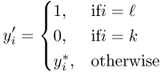
Then, prove that $images$ , where $images$ and $images$ are the objective function values of the solutions $images$ and $images$ , respectively. This would contradict the assumption that $images$ is optimal and thus complete the proof.

Show that this approach does not work by creating a set $images$ (with $images$ , $images$ , and the elements sorted in increasing order of $images$ ) and a solution $images$ such that:
- $images$
- $images$ , $images$ for some $images$
- If we define $images$ as above, then $images$ .
12.5 (Nonclosest Assignments in LMRP) Consider the 3‐node instance of the LMRP pictured in Figure 12.5. Each circle represents a retailer, and each retailer is eligible to be converted to a DC. The numbers on the links indicate the transportation cost ( $images$ ) between retailers; the transportation cost between a retailer and itself is 0. Construct an example, using this instance, for which there is a retailer in the optimal solution that is assigned to a DC that is not its closest open DC. That is, this problem is asking you to choose values for the parameters ( $images$ , $images$ , $images$ , $images$ , etc., but not including $images$ since those are given in the diagram) and demonstrate that in the optimal solution, there is a retailer assigned to a given DC, even though there is another open DC that is closer. You do not need to enumerate the objective value of every possible solution, but you should argue rigorously that your candidate solution is optimal.

Figure 12.5 3‐Node LMRP instance for Problem 12.5.
12.6 (LRP with Distance Constraints) In this problem, you will extend the location–routing problem (LRP) to consider distance constraints on the length of the vehicle routes, and you will reformulate the model as a set partitioning problem . In addition to the notation in Section 12.3, let be the distance between nodes i and j, and let be a prespecified upper bound on the total distance of each route. Let be the set of all feasible routes from depot . As in Section 12.3, a route is only feasible if it begins and ends at the same depot and does not violate its capacity, and now we also require it to satisfy the distance constraint. Let be the cost of route , which equals the sum of the costs of the edges on the route. Let be a parameter that equals 1 if route visits customer i, and 0 otherwise.
The model aims to choose one route $images$ for each $images$ to minimize the total cost of the routes. Every customer must be included in exactly one route. The objective function consists of the total fixed cost of opening depots plus the total routing cost. As before, $images$ is a decision variable that equals 1 if depot $images$ is opened, and now let $images$ be a new decision variable that equals 1 if route $images$ is selected and 0 otherwise. You may assume there is no upper bound on the number of depots open or the number of vehicles assigned to each depot.
1. Formulate the LRP with distance constraints as a linear integer programming problem. If you introduce any new notation, define it clearly. Explain the objective function and constraints in words.
2. Design a heuristic for the LRP with distance constraints that is based on the greedy‐add heuristic we discussed for the UFLP in Section 8.2.5. Write pseudocode for your heuristic. You may assume that your heuristic has access to the following two black‐box functions and may use them as many times as you wish. (“Black‐box” means you don't know how the functions work, but you may call them and use their results.)
  - Route_Enumerate(j,I) takes as input a candidate depot location j and a customer set I and returns as output the set $images$ of all feasible routes for depot j. The function also returns, for each route $images$ , the values of the parameters $images$ and $images$ .
  - Route_Select(j,I) takes as input a candidate depot location j and a customer set I and returns as output a set $images$ , which contains the lowest‐cost subset of all feasible routes for depot j such that every customer in I is visited by exactly one route. The function also returns, for each route $images$ , the values of the parameters $images$ and $images$ .
  Note that in both functions, the input parameter I may equal the entire customer set or only a subset of it.

Note

..................Content has been hidden....................

You can't read the all page of ebook, please click here login for view all page.