11.1.1 Overview

The vehicle routing problem (VRP) is concerned with optimizing a set of routes, all beginning and ending at a given node (called the depot ), to serve a given set of customers. The VRP was first introduced by Dantzig and Ramser (1959). It is a multi‐vehicle version of the traveling salesman problem (TSP), and is therefore more applicable in practice since most organizations with substantial delivery operations use multiple vehicles simultaneously. Of course, it is also more difficult than the TSP since it involves decisions about how to assign customers to routes, in addition to how to optimize the sequence of nodes on each route. As a result, today's “hard” VRP instances tend to involve, say, hundreds of nodes, whereas hard instances of the TSP involve thousands or tens of thousands of nodes.

Figure 11.1 shows the optimal solution to a VRP instance called eil51 from the TSPLIB data set repository (Reinelt, 1991) and originally from Christofides and Eilon (1969). The depot is near the center of the region, marked by a square, while the customers are drawn as circles. Each node has a coordinate in , and the distances between pairs of nodes are Euclidean. The demands range from 3 to 41, and the vehicle capacity is 160. Note that the optimal VRP solution involves routes that cross each other. Of course, just as in the TSP, it is never optimal for an individual route to cross itself if the distances are Euclidean, since each individual route in a VRP solution is a TSP tour on the nodes in the route.

The VRP is used to model less‐than‐truckload (LTL) deliveries, in which a single vehicle delivers goods to multiple customer nodes before returning to the depot. In contrast, the facility location models in Chapter 8 assume truckload (TL) deliveries, in which a vehicle delivers to only a single node. In addition to differences in the shape of the delivery routes, TL and LTL shipments have different cost structures for shippers. Typically, when a firm ships products TL, it pays a fixed cost for the shipment; the fixed cost depends on the origin and destination points, but not on the quantity of goods being shipped. In contrast, LTL shipments are charged based on weight or volume, as well as on origin and destination. Companies such as FedEx and UPS are LTL carriers.

Not surprisingly, the VRP is an immensely important problem for such carriers. For example, UPS's route‐optimization system, called On‐Road Integrated Optimization and Navigation (ORION), saves the company an estimated $300–$400 million per year and is sometimes described as the world's largest operations research project (Holland et al., 2017). UPS and ORION won the prestigious INFORMS Edelman Award in 2016. (See Case Study 11.1.)

We will formulate the VRP in Section 11.1.3, and then discuss exact and heuristic algorithms in Sections 11.2 and 11.3, respectively. For a more thorough discussion of the VRP, see the reviews by Laporte and Nobert (1987), Laporte (1992b), Laporte et al. (2000) and Cordeau et al. (2002), among others, and the books by Toth and Vigo (2001a) and Golden et al. (2008). Several web sites compile data sets and other useful information about the VRP, including the VRP Repository ¹ and the NEO Research Group at the University of Malaga. ²

11.1.2 Notation and Assumptions

We are given a set of nodes and a symmetric distance matrix that satisfies the triangle inequality. Node 0 is the depot. Let be the set of customer nodes. Each node has a demand , with . For , let

Some of the models and algorithms we consider below will assume that there are exactly K vehicles available at the depot, and that all of them must be used, while others allow the number of vehicles to be unrestricted. In either case, we assume that the vehicles are all identical, each with a capacity of C. We assume that for all ; otherwise, the problem is infeasible.

Other capacity‐type constraints are sometimes used instead of, or in addition to, vehicle capacities. For example, in some models, the total distance or time that a vehicle travels is constrained. (If there were no capacity‐type constraints and the distances satisfy the triangle inequality, then the VRP would be equivalent to the TSP —why?) The problem we consider is sometimes called the capacitated vehicle routing problem (CVRP) to distinguish it from models with these other types of constraints, but we will refer to the problem simply as the VRP.

Many variations of this basic setup are possible. For example, the vehicles may be nonidentical in terms of their capacities or other constraints, or we may incur a fixed cost for each vehicle used. There are more complex extensions, as well, such as:

• Time windows during which vehicles must arrive at each customer.
• Multiple depots that nodes may be served from, with the assignment of nodes to depots a decision variable.
• Backhauls, in which some customers require product to be delivered, others require product to be picked up and brought back to the depot, and delivery customers must come before backhaul customers on a given route.
• Pickups and deliveries , in which customers require their shipment to be picked up at one location and delivered to another, both by the same vehicle.
• Periodic models in which a given customer must be visited a fixed number of times per week (or month, etc.).

We will discuss some of these variants and extensions in Section 11.5.

11.1.3 Formulation of the VRP

As in the TSP, we will define a decision variable that equals 1 if a route goes from i to j or from j to i, for . For the depot, we allow , where indicates a single‐customer route. (If single‐customer routes are prohibited, we can simply require .) The decision variables are defined only for , but, as with the TSP, we will often omit the requirement when writing summation and constraint indices.

In this section, we assume that exactly K vehicles must be used to serve the nodes in . For a subset , let be the minimum number of vehicles required to serve all nodes in S. We discuss the calculation of below.

The VRP can be formulated as an integer programming (IP) model as follows:

(11.1)

(11.2)

(11.3)

(11.4)

(11.5)

(11.6)

(This is a slightly less general version of the formulation presented by Laporte et al. (1985).) The objective function 11.1 calculates the total length of the routes. Constraints 11.2 require exactly two edges to be incident to each node except the depot, and constraint 11.3 requires edges to be incident to the depot. Constraints 11.4 are called capacity‐cut constraints (or sometimes just capacity constraints); they are a generalization of subtour‐elimination constraints. Equivalently, we could use either

(11.7)

or

(11.8)

Constraints 11.5 and 11.6 enforce the integrality and bounds on the . This formulation is known as a two‐index formulation since the decision variables each have two indices.

This formulation is remarkably similar to the TSP formulation (10.7)–(10.10), despite the fact that the VRP allows multiple routes (and must ensure that each is connected to the depot) and has capacity restrictions. The capacity‐cut constraints 11.4 do quite a bit of heavy lifting, ensuring both the depot‐connectedness and the capacity‐feasibility of every route. To see this, suppose first that there is a route that is not connected to the depot—in other words, a subtour. Let S be the nodes on this route. Then the number of edges contained within S (the left‐hand side of 11.4) equals , which violates 11.4 since . Now suppose that there is a route that violates the capacity constraint. Again, let S be the nodes on this route, excluding the depot. Then , but since the route is over capacity, and 11.4 is violated.

The question remains how to calculate . An exact calculation of requires solving the bin‐packing problem. In the bin‐packing problem, we are given a set of objects, each with a given weight (or other measure of size). The objective is to “pack” the objects into bins, each of which has a fixed capacity, minimizing the total number of bins used. Therefore, is equal to the optimal objective value of the bin‐packing problem for a set S of objects of weight and bins of capacity C. Unfortunately, the bin‐packing problem is NP‐hard , so it is common to replace with a lower bound; one easy bound is

(11.9)

In fact, replacing with the lower bound 11.9 in the capacity‐cut constraints 11.4 or 11.7 retains the validity of the IP formulation (Cornuejols and Harche, 1993), though it weakens its LP relaxation. Obviously, whether we use 11.9 or the bin‐packing problem, it is impractical to calculate for all since there are exponentially many such sets. Then again, it is impractical to enumerate all of the capacity‐cut constraints 11.4 anyway; so can be calculated as needed when a given constraint is added.

The two‐index formulation 11.1–11.6 is simple but fairly inflexible. Although one could look at a solution and assign trucks to routes or determine the sequence of nodes on the route, the model itself is not “aware” of these attributes endogenously. Because of this, it cannot be modified to handle time windows, precedence constraints, nonidentical vehicle capacities or capabilities, sequence‐dependent costs, or a range of other realistic problem features.

To correct this, we can use a three‐index formulation that explicitly keeps track of which vehicle is assigned to each route. In particular, if vehicle k travels directly from i to j, and 0 otherwise. Note that, unlike in the two‐index formulation , the x variables indicate which node (i or j) comes before the other. Therefore, is defined for all , not just for . We also have a binary variable that equals 1 if vehicle k serves node i and 0 otherwise, for . This gives us the following formulation, which is based on the formulation by Fisher and Jaikumar (1981):

(11.10)

(11.11)

(11.12)

(11.13)

(11.14)

(11.15)

(11.16)

(11.17)

The objective function 11.10 calculates the total route length. Constraints 11.11 require every nondepot node to be served by exactly one route. Constraint 11.12 requires the depot to be contained on K routes. (This constraint can be removed if K is an upper bound on the number of vehicles but not all K vehicles need to be used.) Constraints 11.13 require to equal 1 if and only if vehicle k traverses exactly one arc into h and one arc out of h. Constraints 11.14 ensure the vehicle capacity is not exceeded. Constraints 11.15 are subtour‐elimination constraints , and 11.16–11.17 are integrality constraints.

This formulation has an explicit capacity constraint 11.14. In the two‐index formulation, in contrast, we cannot calculate the total load on a given vehicle endogenously, so capacity constraints must be imposed via the parameter in the capacity‐cut constraints 11.4. The three‐index formulation can easily handle vehicle‐dependent capacities: We simply change the right‐hand side of 11.14 to , where is the capacity of vehicle k.

The three‐index formulation is more difficult to solve than the two‐index formulation since there are many more binary variables ( vs. ), but the added complexity is often compensated for by the increased flexibility. In addition, a three‐index model can be converted to a two‐index model by setting ; therefore, any valid inequalities developed for the two‐index formulation are also valid for the three‐index formulation.

11.2.1 Dynamic Programming

Eilon et al. (1971) propose a dynamic programming (DP) algorithm for the VRP. Whereas the DP for the TSP acts recursively on the nodes, the VRP algorithm acts recursively on the routes, expressing the optimal distance for a solution that uses k routes in terms of the distance using routes.

For a subset , let be the length of the optimal TSP tour through the depot and the nodes in S if and otherwise. Define as the minimum possible total distance to deliver to the nodes in S using k routes, or if the nodes in S cannot be feasibly served by k routes. If , then . Suppose . If we know that one of the k routes serves a customer set , then the optimal distance is given by , where the second term computes the length of the route through and the first computes the lengths of the remaining routes. Therefore, we can calculate recursively:

(11.18)

If the number of vehicles is fixed to K, then the total length of the optimal VRP solution is given by . If the number of vehicles is unrestricted, we can choose the k that minimizes .

Of course, this is not a computationally efficient way to solve the VRP. Not only do we need to enumerate all subsets of , and all subsets of those sets, and so on, but we must also solve the TSP for each of those subsets. One alternative is to “relax” the state space in such a way that the resulting recursion provides a lower bound on the optimal VRP objective function value. For example, we can define the DP recursion in terms of the load represented by the customers in S rather than in terms of the customers themselves. Let be the optimal distance to use k vehicles to deliver to a set of nodes whose total demand equals d, or if , i.e., if k vehicles are not sufficient to serve a total demand of d. Let be the length of the optimal TSP tour through the depot and a set of nodes with total demand d, or if . (Actually, calculating an exact value for is itself difficult, so in practice one can replace by a lower bound on it; see Christofides et al. (1981).) Note that for any S,

(11.19)

since the optimal TSP tour through , which has length , is a feasible solution for the problem of finding the optimal tour through the depot and a set of nodes with total demand .

A recursion for is given by

(11.20)

The significance of this relaxation is given by the following proposition.

This technique is known as state‐space relaxation. It was introduced by Christofides et al. (1981), who also introduce several other recursions and relaxations that provide tighter bounds than 11.20. This lower‐bounding procedure can be embedded into a branch‐and‐bound algorithm.

11.2.2 Branch‐and‐Bound

Because the VRP formulations in Section 11.1.3 have an exponential number of constraints, most branch‐and‐bound algorithms relax the capacity‐cut constraints and solve the resulting problem to obtain lower bounds on the optimal objective function value. For example, suppose we relax the capacity‐cut constraints 11.4 in the two‐index VRP formulation to obtain the following formulation:

(11.22)

(11.23)

(11.24)

(11.25)

Constraints 11.23 combine constraints 11.2 and 11.3 by defining

The model formulated in 11.22–11.25 chooses the minimum‐cost set of edges such that every node h has degree . This is known as the b‐matching problem and is a generalization of the 2‐matching problem ; it can be solved efficiently (Miller and Pekny, 1995). The b‐matching problem only provides a lower bound since its solutions may be infeasible for the VRP due to capacity violations or routes that are disconnected from the depot. Miller (1995) proposes a branch‐and‐bound algorithm based on this b‐matching relaxation.

Another relaxation, due to Fisher (1994a), extends the notion of 1‐trees (Section 10.6.1) to the VRP. He defines a K‐tree as a minimum‐cost set of edges that contains every node, and he further focuses on K‐trees in which the depot has degree . In every VRP solution there are edges and the depot has degree , and so the problem of finding an optimal degree‐constrained K‐tree is a relaxation of the VRP. This degree‐constrained K‐tree problem can be formulated as follows:

(11.26)

(11.27)

(11.28)

(11.29)

Constraints 11.27 enforce the degree restriction on the depot, while constraints 11.28 ensure connectivity (at least one edge comes out of every subset). (This model prohibits single‐customer routes, hence constraints 11.29 apply to the depot, as well.) This formulation can be seen as a relaxation of 11.1–11.6 by removing constraints 11.2, using 11.7 in place of 11.4 and replacing its right‐hand side with 1 (which is always less than ). Fisher (1994b) shows that this problem can be solved in time. Fisher (1994a) uses this lower bound in a branch‐and‐bound algorithm.

Unfortunately, neither the b‐matching bound nor the K‐tree bound is very tight, often falling 20% or more below the optimal VRP objective value (Toth and Vigo, 2001b). Therefore, branch‐and‐bound methods based on these and other simple relaxations are generally not effective for any but the smallest problem instances.

11.2.3 Branch‐and‐Cut

Recall from Section 10.3.3 that a branch‐and‐cut algorithm involves relaxing certain constraints (integrality and/or functional constraints), solving the resulting problem, and then adding additional constraints (“cuts”) that make the current optimal solution infeasible, thus tightening the formulation. One obvious choice for VRP constraints to relax is the capacity‐cut constraints , which in this section we will assume are in the form given in 11.7, that is:

As we discussed in Section 11.2.2, relaxing the capacity‐cut constraints results in the b‐matching problem , which can be solved efficiently. The question, then, is how to solve the separation problem —how to identify a violated inequality (a cut) that will render the solution to the relaxed problem infeasible.

The answer turns out to depend on how tight we wish the capacity‐cut constraints to be. It is difficult to identify violated inequalities of the form 11.7, since calculating itself is NP‐hard due to its relationship to the bin‐packing problem . Ralphs et al. (2003) propose a heuristic for solving the separation problem in this case. On the other hand, we noted in Section 11.1.3 that the formulation is still valid if we replace by . The separation problem in this case is still difficult, but less so—it is still usually done heuristically. We can even replace by the weaker value , which does not maintain the validity of the IP formulation but is more tractable. The separation problem for this form of the constraints can be solved in polynomial time (McCormick et al., 2003).

Since the VRP is a generalization of the TSP , any valid inequality developed for the TSP—for example, those discussed in Section 10.3.3—can be adapted for the VRP (Naddef and Rinaldi, 1993). On the other hand, cuts derived in this way are often not particularly tight for the VRP, since these inequalities ignore the vehicle capacity. They can be strengthened by making use of the function —in essence, combining the capacity‐cut inequalities (which account for the bin‐packing aspect of the VRP) with the TSP‐derived inequalities (which account for the routing aspect).

We illustrate this idea using comb inequalities. Recall from Section 10.3.3 that a comb consists of a set H called the handle and a collection of sets called teeth, such that each contains at least one node in H and one node not in H and such that s is odd and at least 3. A comb inequality for the TSP can be written as in (10.16), that is:

To adapt this for the VRP, Laporte and Nobert (1984) prove the following:

If , then for all k, and 11.30 is identical to (10.16) for the TSP. Theorem 11.1 can be adapted to the case in which the depot is contained in one of the teeth, as well.

Another approach to adapting TSP comb inequalities for the VRP is as follows. Suppose we duplicate the depot so that there are K copies; call this set of depots D. Let if . Then a TSP tour through is a feasible VRP solution if the total demand of the nodes between consecutive visits to depot nodes is no greater than . A TSP comb inequality on can be converted to a VRP comb inequality by re‐combining the nodes in D back into the single depot, but we must adapt the definition of a comb to deal with the fact that the teeth may now intersect (because multiple teeth may contain the depot). Assume that for some , teeth do not intersect, and teeth intersect only at the depot. Assume also that for all ; in other words, if tooth contains the depot, then the nodes not in the tooth require all K vehicles to serve them. Then one can show (see Problem 11.12) that the following inequality is valid for every VRP solution through N:

(11.31)

This inequality can be tighter than 11.30.

For a more thorough review of branch‐and‐cut approaches for the VRP, see Naddef and Rinaldi (2001).

11.2.4 Set Covering

Because VRP solutions consist of a set of disjoint routes, the VRP lends itself well to a set covering/column generation approach, similar to the approach in Section 12.2.7 for the LMRP and described further in Section D.2.4. This method was proposed by Balinski and Quandt (1964) and has since been refined by a number of other authors; see, e.g., Bramel and Simchi‐Levi (2001) for an overview. (Another set of classical approaches, called petal heuristics, can be thought of as a simplified and approximate version of the set covering/column generation approach in which routes are generated heuristically; see, e.g., Foster and Ryan (1976) and Renaud et al. (1996).)

Suppose for a moment that we could enumerate all feasible routes, i.e., routes that begin and end at the depot, visit each customer at most once, and do not violate the capacity constraint. Let be the set of all feasible routes; for a given route , let be the total length of the route; and let if i is on route r, 0 otherwise. Define a decision variable , for , as follows:

The set covering formulation for the VRP is as follows:

(11.32)

(11.33)

(11.34)

(11.35)

The objective function 11.32 calculates the total distance of the routes chosen. Constraints 11.33 require each node to be contained in a chosen route. Constraint 11.34 requires at most K routes to be used. (Here, we treat K as an upper bound on the number of routes.) Constraints 11.35 are integrality constraints. Note that, although constraints 11.33 are written as inequality constraints, they will always hold as equalities in the optimal solution. (Why?)

Of course, is exponentially large, so it is not practical to enumerate all feasible routes for even moderately sized instances. Therefore, the set covering algorithm begins by enumerating only a (relatively small) subset of feasible routes. This can be done randomly, or using some heuristic. Let (VRP‐SC') be the problem (VRP‐SC) restricted to , and let (VRP‐SC′¯) be its LP relaxation. Since is not too large, (VRP‐SC′¯) is relatively easy to solve using a standard LP solver. Let be the optimal solution to (VRP‐SC′¯). How can we tell whether is optimal for (VRP‐SC¯) (the LP relaxation of the original problem, with the full set )?

To answer this question, we'll formulate the dual of (VRP‐SC¯), letting be the dual variables corresponding to constraints 11.33 and be the dual variable for 11.34:

(11.36)

(11.37)

(11.38)

(11.39)

Let be the optimal dual values corresponding to the optimal primal solution for (VRP‐SC′¯). If is feasible for (VRP‐SC‐D¯), then it is optimal for (VRP‐SC‐D¯) (why?) and is optimal for (VRP‐SC¯). Thus, checking optimality of for (VRP‐SC¯) is equivalent to checking feasibility of for (VRP‐SC‐D¯). But checking feasibility is not straightforward, since (VRP‐SC‐D¯) has an exponential number of constraints, most of which we have not enumerated.

The solution to this challenge is to look explicitly for a violated constraint, i.e., for an such that

(11.40)

or, equivalently, such that where

is the reduced cost of column r. In other words, we want to solve the following column generation problem:

(11.41)

(11.42)

This problem searches for the tour that minimizes . If the optimal is negative, then we have found a constraint that violates, and moreover, we have found a new column that we should add to . If the optimal is nonnegative, then we have proven that is optimal for (VRP‐SC¯).

Now the question is how to solve . This problem itself is NP‐hard, because for a given route r, even evaluating requires finding an optimal TSP tour through the nodes on the route. It is usually solved using branch‐and‐bound or branch‐and‐cut (Agarwal et al., 1989; Desrochers et al., 1992; Bixby, 1998).

Even after doing all of this, we have still only solved the LP relaxation of (VRP‐SC). To solve (VRP‐SC) itself, one approach is to use as a starting point in a branch‐and‐price algorithm to solve (VRP‐SC) exactly. In this approach, new columns are generated as needed within the branch‐and‐bound tree, with the net result of solving (VRP‐SC) without enumerating all of the columns in explicitly. See Desrochers et al. (1992) for an algorithm of this type.

Another approach is to solve (VRP‐SC') exactly with the current set of columns, i.e., solving the VRP restricted to the routes in , by branch‐and‐cut or another method (see, e.g., Bramel and Simchi‐Levi (2001)). Since we are not solving the full problem to optimality, this approach is a heuristic.

Both methods are quite effective, in large part due to the fact that the LP relaxation of the set covering problem tends to be very tight; in fact, it often has all‐integer solutions. (We made a similar observation about the uncapacitated fixed‐charge location problem (UFLP) on page 272.) This has been observed empirically (e.g., Desrochers et al., 1992), and in fact Simchi‐Levi et al. (2013) prove that the LP bound for the set covering formulation of the VRP approaches the IP value asymptotically as . Bramel and Simchi‐Levi (1997) prove this for the more general VRP with time windows.

The set covering/column generation algorithm is summarized in Algorithm 11.1.

11.3.1 The Clarke–Wright Savings Heuristic

The Clarke–Wright savings heuristic (Clarke and Wright, 1964) is one of the best‐known heuristics for the VRP. The heuristic assumes that the number of vehicles is unrestricted. It begins by placing each node on its own route and then merging routes when doing so reduces the total distance.

Consider the two routes shown in Figure 11.2(a). Suppose we were to merge the two routes by adding an edge from node i to node j, as shown in Figure 11.2(b). The savings from such a merger is given by

(11.43)

By the triangle inequality, .

The savings heuristic builds a savings list of the values for all , sorted in descending order. The algorithm then proceeds down the list, implementing, at each iteration, a merger of two routes at nodes i and j if the following conditions hold:

1. i and j are on different routes.
2. i and j are both adjacent to the depot on their respective routes.
3. The resulting route would be feasible with respect to capacity constraints.

Once a merger has been considered and either implemented or rejected, it is never considered again, since none of the conditions above change from false to true during the course of the heuristic. The algorithm terminates when every merger has been considered. Pseudocode for the heuristic is given in Algorithm 11.2.

The Clarke–Wright solution to the eil51 instance in Figure 11.1 has a total distance of 582 (compared to the optimal distance of 521) and is pictured in Figure 11.5.

A variant of the savings heuristic skips the sorting step (line 4) and instead implements mergers with positive savings in the order in which they are found. Laporte and Semet (2001) refer to this variant and the version in Algorithm 11.2 as the sequential and parallel versions, respectively. (Alternate terms might be first‐improving and best‐improving. ) They report that the parallel version outperforms the sequential version considerably and warn that some authors neglect to indicate which version they are using when reporting computational results.

On the other hand, it is sometimes worthwhile to consider mergers other than the one with the largest savings through a randomization mechanism. For example, we might choose randomly from among the best feasible mergers to obtain a solution; we can repeat this several times, possibly with different values of , and choose the best solution found. Daskin (2010) proposes an approach like the one listed in Algorithm 11.3. L is called the randomization depth and M is called the randomization iterations; both are inputs to the algorithm and are typically small, say, .

Sometimes route mergers are selected using a matching algorithm ; see, e.g., Desrochers and Verhoog (1989) and Wark and Holt (1994). These methods tend to be a bit more accurate than the classical Clarke–Wright algorithm but also significantly slower.

Another variant, proposed by Gaskell (1967) and Yellow (1970), uses a generalized savings calculation,

where is a route shape parameter that allows the user to specify how much emphasis to place on the distance between the two nodes to be merged. If is large, mergers are penalized if i and j are far from each other. This tends to encourage more compact routes.

11.3.2 The Sweep Heuristic

The sweep heuristic (Wren, 1971; Wren and Holliday, 1972; Gillett and Miller, 1974) builds clusters of nodes by rotating a ray emanating from the depot, adding nodes as the ray hits them, and beginning a new cluster when the next node would violate the vehicle capacity. Routes are then constructed by solving a TSP (exactly or heuristically) for each cluster. Typically, the number of routes is unrestricted. In the pseudocode for the sweep heuristic in Algorithm 11.4, represents the polar coordinates of node , and represents cluster k of nodes.

Routes produced by the sweep heuristic never overlap, but optimal routes often do. Therefore, node‐exchange improvement heuristics (see Section 11.3.4) can be particularly useful after the heuristic completes its execution.

The sweep heuristic is an example of a two‐phase method in which clustering and routing are done in two separate steps. Two‐phase methods come in two types: cluster‐first, route‐second and route‐first, cluster‐second. The sweep method is an example of the former type, ³ as is the location‐based heuristic discussed in Section 11.3.3. In contrast, route‐first, cluster‐second methods solve a TSP on the entire node set and then partition the tour into routes (Beasley, 1983). Laporte and Semet (2001) observe that these methods rarely perform better than cluster‐first, route‐second approaches, and Li and Simchi‐Levi (1990) provide a theoretical justification.

For the eil51 instance in Figure 11.1, the sweep heuristic returns the solution pictured in Figure 11.7, which has a total distance of 586.27. (The routes were optimized using the farthest insertion heuristic rather than with an exact algorithm.)

11.3.3 The Location‐Based Heuristic

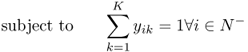
The location‐based heuristic (LBH) of Bramel and Simchi‐Levi (1995) approximates the VRP by the capacitated concentrator location problem (CCLP) , a close variant of the capacitated facility location problem (CFLP) with single‐sourcing constraints (Section 8.3.1) in which the demands are ignored in the transportation costs but not in the capacity constraints. The basic idea is to use the CCLP to cluster the nodes and then solve TSPs to optimize the individual routes; see Figure 11.8. The facilities opened in the CCLP solution are called “seed nodes.” The choice of seed nodes is actually rather inconsequential; what is important is the cluster of nodes that are assigned to each seed node (including the seed node itself), since these will form the node sets for the individual routes. The heuristic assumes that the number of routes is unrestricted.

We will assume that the sets of customers and potential facility locations (called I and J in the CFLP) are both equal to . We would like the cost of locating a facility at node j and serving a set of customer nodes in the CCLP to approximate the cost (length) of a TSP tour through the depot and the nodes in . The LBH divides the cost of this tour into two components, the portion to and from the depot and the portion among the other nodes. It includes the length of the former portion in the fixed location cost and that of the latter portion in the transportation costs . ⁴ In particular, for each , we set

(11.45)

and for each , we set as either

(11.46)

or

(11.47)

If we locate a facility at node j, then 11.46 approximates node i's contribution to the TSP tour length as the distance from j to i and back, while 11.47 approximates it using the cost to insert node i into the tour that goes from the depot to node j and back. Bramel and Simchi‐Levi (1995) refer to 11.46 as the star connection cost and to 11.47 as the seed tour cost. We'll use LBH‐SC and LBH‐ST to refer to the LBH heuristic using these two costs, respectively. Neither is meant to model the TSP tour cost exactly; the aim is simply to find costs for the CCLP that tend to produce solutions that translate to good solutions for the VRP. The computational tests by Bramel and Simchi‐Levi (1995) suggest that LBH‐ST performs somewhat better computationally, but LBH‐SC has nice theoretical properties; see Theorem 11.3 below.

Given these costs, we can formulate the CCLP:

(11.48)

(11.49)

(11.50)

(11.51)

(11.52)

(11.53)

can be solved using any available method; Bramel and Simchi‐Levi (1995) suggest using the Lagrangian relaxation method described in Section 8.3.1, calculating by solving a 0–1 knapsack problem . To find feasible (upper‐bound) solutions to the CCLP, they open facilities in order of , and for each new facility, they assign customers by solving a new knapsack problem on the customers that have not yet been assigned.

Once we have solved the CCLP, we construct clusters of nodes, each of which consists of the nodes assigned to a given seed node in the CCLP solution. We then solve a TSP on the nodes in each cluster, either exactly or approximately. The LBH is summarized in Algorithm 11.5.

An earlier heuristic, by Fisher and Jaikumar (1981), is similar in spirit to the LBH, but instead of clustering via a facility location problem, it does so by solving a generalized assignment problem. Fisher and Jaikumar (1981) report good computational results for their algorithm, but the results have been difficult to replicate (Cordeau et al., 2002).

The LBH‐SC heuristic is asymptotically optimal as the number of nodes increases. In other words, as , the total distance of the solution returned by the LBH‐SC heuristic approaches the optimal VRP distance.

Before proving the asymptotic optimality of LBH‐SC, we return to the connection between the VRP and the bin‐packing problem. Recall that, in the bin‐packing problem, we are given a set of objects, each with a given weight (or other measure of size). The objective is to “pack” the objects into bins, each of which has a fixed capacity, minimizing the total number of bins used. Let be the minimum number of bins of capacity that are needed to pack n objects whose weights are drawn from a given probability distribution. It is well known that converges to a constant as n increases:

where is a constant (known as the bin‐packing constant ) that depends on the probability distribution of the weights.

Suppose the demands in the VRP are drawn from a given probability distribution. Then the problem of minimizing the number of trucks of capacity required to serve n nodes (ignoring the routing aspect) is equivalent to the bin‐packing problem, and the minimum required number of trucks is , which can be approximated by for large enough n. Bramel et al. (1992) use this fact to characterize the asymptotic behavior of the optimal VRP objective function value:

In other words, for sufficiently large n, can be approximated by , the cost of using vehicles and sending each to a node at a distance of from the depot. This approximate value depends on (which, in turn, depends on the demand distribution and vehicle capacity) and the expected distance from the depot to the nodes.

Let be the total distance of the VRP solution returned by LBH‐SC. First note that this distance is bounded above by , the optimal CCLP cost:

We are now ready to prove that the LBH‐SC heuristic is asymptotically optimal.

There is only limited computational evidence concerning the LBH's performance. Bramel and Simchi‐Levi's (1995) computational results suggest that the LBH is slower and less accurate than other heuristics (see also Cordeau et al., 2002), and few, if any, other computational studies have been published. However, the heuristic has significant theoretical interest, especially in light of Theorem 11.3.

11.3.4 Improvement Heuristics

Since a solution to the VRP consists of multiple TSP‐type tours, any improvement heuristic for the TSP (Section 10.5)—2‐opt, Or‐opt, US, etc.—can also be applied to the routes in a VRP solution.

Another important class of improvement heuristics for the VRP involves moving one or more nodes from one route to another. One simple approach searches for an individual node that can be moved to a different route to reduce the total route length (as in Figure 11.11), and repeats this process until no further exchanges can be found. We can generalize this considerably to identify multiple consecutive nodes that can be moved to another route—or exchanged with nodes on that route—to reduce the total length; see, e.g., Thompson and Psaraftis (1993) and Laporte and Semet (2001).

11.3.5 Metaheuristics

In the past few decades, a class of heuristics called metaheuristics has become very popular, especially for solving combinatorial optimization problems. Metaheuristics are usually quite general and can therefore apply to a wide range of problems but require customization to do so. At the core of a metaheuristic is usually one or more simpler heuristic “moves” (e.g., adding, dropping, or swapping nodes), and these simpler heuristics are manipulated by the metaheuristic itself—hence, “meta.” Many metaheuristics are inspired by natural phenomena, such as the inheritance of genes, the behavior of ant colonies, the flocking of birds, and the heating and cooling of metals. These heuristics attempt to mimic nature's success in achieving certain goals by modeling their behavior algorithmically. Many incorporate randomness, just as in nature.

Classical heuristics such as insertion heuristics for the TSP (Sections 10.4.1–10.4.5), the Clarke–Wright heuristic for the VRP (Section 11.3.1), or the neighborhood search heuristic for the UFLP (Section 8.2.5) usually progress in a single direction to find a solution (though they may be randomized, seeded with different initial solutions, etc., to develop alternate solutions). In contrast, metaheuristics contain explicit mechanisms to explore more regions of the solution space, usually by allowing the search to move in directions toward inferior, or even infeasible, solutions, in the hope of then moving toward an even better solution. (Think of a mountain climber standing halfway up the shorter of two neighboring mountains; she has to go lower, first, before climbing the higher mountain.) One category of metaheuristic, called population search, diversifies the search by considering many solutions at a time, while another, called local search, does so by devoting more computational effort to improving one, or a few, solutions at a time. Because metaheuristics search harder than classical heuristics, they often produce better solutions, as well as longer computation times.

Because the VRP is so difficult to solve exactly, metaheuristics have become one of the most popular, and successful, approaches for solving them. In this section, we discuss two such methods—tabu search and genetic algorithms . For more thorough reviews of these and other metaheuristics for the VRP, including simulated and deterministic annealing , ant colony optimization , and neural networks , we refer the reader to Gendreau et al. (2001) and Vidal et al. (2013). For an overview of metaheuristics in general, see Blum and Roli (2003), Gendreau and Potvin (2010), and Luke (2013).

The success of a given metaheuristic depends heavily on a number of factors, including how it is customized for the optimization problem at hand, how it is implemented in code, and how the user sets the parameters that control its execution. This makes it difficult to compare metaheuristics to one another in general without focusing on the specific details of individual researchers' implementations. Nevertheless, tabu search is generally considered to be the most successful metaheuristic at solving VRP problems and their extensions (Gendreau et al., 2001; Cordeau and Laporte, 2005). This is not to discount other metaheuristics, however—a winning simulated annealing heuristic or genetic algorithm may be just one innovation away.

11.3.5.1 Tabu Search

A tabu search heuristic (Glover, 1986,1989,1990), sometimes called taboo search, uses one or more “moves” to iterate from one solution to the next. A move is sometimes made even if it degrades the solution (or makes it infeasible), and therefore the algorithm needs a way to prevent the search from moving right back to the original solution at the next iteration. One way to do this would be simply to maintain a list of all the solutions encountered thus far and to prohibit moves that would return to one of these solutions, but this would entail an unacceptable memory and computational burden. Instead, tabu search maintains a tabu list of moves that are prohibited (“taboo”) for a certain number of iterations. The moves on the tabu list are the reverse of the moves that were recently implemented. Many tabu search heuristics also incorporate diversification mechanisms to encourage new areas of the search space to be explored (e.g., by penalizing moves that have been made too many times already) and intensification mechanisms to improve promising solutions even further (e.g., by performing improvement heuristics on them). For general references on tabu search, see, e.g., Glover and Laguna (1997), and for its application to the VRP, see, e.g., Cordeau and Laporte (2005).

Perhaps the most critical decision to make when designing a tabu search heuristic is how to define the neighborhood of a given solution, that is, the set of solutions that can be reached from that solution via an allowable move. In the context of the VRP, a simple neighborhood might consist of all solutions that can be reached from the current solution by moving a node from its current route to a new one. The two most common moves for VRP tabu search algorithms are more flexible and powerful than this simple one.

The first is a ‐interchange (Osman, 1993), which consists of moving nodes from route A to route B and nodes from route B to route A, where for a fixed integer . (See Figure 11.12.) If or equals 0, then we are simply moving one or more nodes from one route to another. The neighborhood of a given solution is defined as all solutions that can be reached from it via a single ‐interchange. Osman's algorithm uses to keep the search manageable. Taillard (1993) adds to this an intensification mechanism in which the routes are optimized using an exact TSP algorithm. His algorithm also decomposes the problem geographically so that the search can be parallelized. Rochat and Taillard (1995) enhance Taillard's (1993) algorithm using a concept that has come to be known as adaptive memory, and the resulting algorithm finds the best known solution for all 14 of the benchmark instances by Christofides et al. (1979).

Moves in the TABUROUTE heuristic (Gendreau et al., 1994) are very simple—they consist of moving only a single node to another route, a special case of 1‐interchanges—but the heuristic compensates for the simple neighborhood structure through a host of other features. Most notably, the insertion of the node into its new route is performed using the GENI heuristic (Section 10.4.5), and intensification occurs via the US heuristic (Section 10.5.3), both by Gendreau et al. (1992). TABUROUTE also allows infeasible solutions to be considered during the search. Solutions are evaluated based on a weighted sum of the usual VRP objective function and terms quantifying the capacity and route‐length constraint violations. The weights on these terms are adjusted dynamically in the algorithm to nudge the search back toward feasibility if it has found only infeasible solutions for a certain number of iterations. Toth and Vigo (2003) propose a TABUROUTE‐like algorithm that automatically eliminates long edges, since these are unlikely to appear in optimal solutions. Their approach, known as granular tabu search , results in shorter run times with a minor degradation in solution quality.

The second main type of move, called an ejection chain (Rego and Roucairol, 1996; Xu and Kelly, 1996), consists of moving nodes from route A to route B, other nodes from B to C, others from C to D, and so on. (See Figure 11.13.) Ejection chains are therefore generalizations of ‐interchanges. This mechanism is used in tabu search heuristics by Xu and Kelly (1996), Rego and Roucairol (1996), and Rego (1998); these heuristics appear not to perform as well as those using ‐interchanges (Cordeau and Laporte, 2005).

11.3.5.2 Genetic Algorithms

A genetic algorithm (GA; Holland, 1992) is a metaheuristic in which solutions to the optimization problem are represented as genes that are passed from one generation to the next. Through a process that mimics natural selection (or survival of the fittest), good solutions are more likely to reproduce, and therefore the population tends to produce fitter and fitter offspring as it evolves.

A GA maintains a current population that consists of multiple chromosomes (or individuals), each of which corresponds to a solution by representing it as a string of genes. In each iteration of the GA, several processes (called operators) act on the current population to create a new one. Common operators include reproduction, in which good solutions from the current generation are copied to the next; crossover, in which information from two “parent” solutions is merged to create one or more “offspring” solutions; and mutation, in which a small number of genes are randomly altered. In many GAs, some or all individuals from the population are also subjected to improvement heuristics ; this approach is sometimes called a memetic algorithm.

Let's return to the uncapacitated fixed‐charge location problem (UFLP; Section 8.2) to see how a simple GA might work. Recall that a solution to the UFLP consists of variables and that indicate whether facility j is open and whether customer i is assigned to facility j, respectively. Once we know the facility locations, the optimal assignments are easy to determine, so it suffices to encode only the variables. This can be done quite simply, by setting the gene for facility j equal to . A small population for a problem with is shown in Figure 11.14(a). Crossover can be performed in a number of ways. One way is to choose a “crossover point,” and to use the genes from parent A before the crossover point and from parent B after the crossover point, as in Figure 11.14(b) (the parents are the second and fourth individuals); this is called one‐point crossover. Another way, called uniform crossover, is to choose a parent randomly and independently with some probability for each gene, as in Figure 11.14(c).

Neither of these approaches works for the VRP, however. To see why, imagine we encode solutions by listing the customer nodes in the order they are visited. (For simplicity, we'll temporarily assume there is only a single route.) Then the offspring produced by simple crossover methods such as one‐point or uniform crossover are likely to contain some nodes twice and some nodes not at all. Figure 11.15 illustrates this for one‐point crossover. GAs for the VRP must therefore use more sophisticated crossover mechanisms to ensure feasibility.

Van Breedam (1996) proposes encoding a solution as a string in which the depot is repeated each time a new route begins. For example, the string represents two routes, and . His crossover mechanism is based on the partially matched crossover (PMX) operator for the TSP and other sequencing problems (Goldberg, 1989). It works by selecting two crossover points and exchanging the strings between them to produce two new offspring. For example, in Figure 11.16, nodes 7 and 3 in parent A are swapped with nodes 6 and 8 in parent B, both between the crossover points and outside of them. He proposes a mutation operator in which two nodes on different routes are swapped, like a ‐interchange operation with .

A more complex, and effective, crossover operator is used in the memetic algorithm by Nagata and Bräysy (2009) and based on the edge assembly crossover (EAX) operator for the TSP (Nagata and Kobayashi, 1997). Given two parents, A and B (Figure 11.17(a)), the operator works as follows:

1. Let be the graph consisting of node set N and edge set , where and are the edges in parents A and B, respectively. That is, contains all the edges from both parents, excluding edges that they have in common. (Figure 11.17(b).)
2. Partition into cycles that consist of alternating edges from parents A and B; these are called ‐cycles.
3. Choose a subset of the ‐cycles; this is called an E‐set. (Figure 11.17(c).)
4. Form an intermediate solution by removing from A all edges that are in the E‐set and replacing them with edges from the E‐set that came from B. The intermediate solution may include subtours. (Figure 11.17(d).)
5. Fix infeasibilities with respect to subtours and capacity constraints using moves similar to 2‐opt and ‐interchange .

Their method allows capacity‐infeasible solutions to diversify the search space (as in a tabu search heuristic) , with a penalty in the objective function to encourage feasibility. A local search procedure improves the solutions found by the GA, again using 2‐opt and ‐interchange‐type moves. The method found new best known solutions on several benchmark instances.

Many more varieties of GA (and the more general category of evolutionary algorithms ) have been proposed for the VRP. For a thorough review, see Potvin (2009). For a general reference on GAs, see, e.g., Goldberg (1989).

11.4.1 TSP‐Based Bounds

Suppose that each customer has a demand of 1, so that C represents the number of customers that each vehicle can serve. Let be the total length of the optimal VRP routes through a set of customers, and let be the length of the optimal TSP tour through the nodes in M. Let , and . Haimovich and Rinnooy Kan (1985) prove the following bounds on :

The upper bound in Theorem 11.4 consists of two parts; the first roughly corresponds to the “radial” distance to travel from the depot to the route, while the second represents the “local delivery” distance once the vehicle has reached the customer area.

Both bounds in Theorem 11.4 are tight—see Problem 11.18. In fact, as , the lower and upper bounds both approach —that is, the VRP approaches the TSP, as we noted in Section 11.1.2.

In the special case in which the customers are uniformly distributed in the unit square and the depot is located at its center, we can approximate using the square‐root approximation (10.41). One can show (Finch, 2003, p. 479) that the expected distance from a random point in the unit square to the center of the square is given by

(11.60)

Therefore, Theorem 11.4 suggests that

(11.61)

for points in the unit square. Here, the notation means “ is greater [less] than or equal to a constant that is approximately equal to a [b].” For fixed C, the approximate bounds diverge as , as shown in Figure 11.19 for . Note that for , the square‐root term in the lower bound dominates the , while for , the linear term does.

11.4.2 Optimal Objective Function Value as a Function of n

Recall from Theorem 10.19 that as n gets large, the optimal TSP tour length increases as . In contrast, the optimal VRP objective function value increases linearly as n gets large. Haimovich and Rinnooy Kan (1985) prove the following:

In other words, for sufficiently large n, can be approximated by , the cost of using vehicles and sending each to a node at a distance of from the depot. (We discussed a similar, but more general, result by Bramel et al. (1992) in Theorem 11.2, which allows the demands to be iid rather than equal to 1.) As we discussed in Section 11.4.1, the first term of the upper bound in Theorem 11.4 is proportional to n and represents the radial distance to travel to the customers from the depot. The second term represents the local delivery distance once we reach the set of customers on the route, and by Theorem 10.19, this term is proportional to as n gets large. Theorem 11.5, then, says that for fixed C, the radial distance dwarfs the local delivery distance as , for itself and not just its upper bound. (See Figure 11.20(a).)

What happens when C increases along with n? The answer depends on the relative rate of increase in the two parameters. Let be the capacity when there are n nodes. Haimovich and Rinnooy Kan (1985) prove that, under certain conditions on the probability distributions, if C increases much more slowly than , then the approximate total distance for large n is still proportional to n, whereas if C increases much more quickly than , then the approximate total distance is proportional to . In other words, as , if the capacity does not keep pace with the square root of the number of nodes, then the number of routes increases and the radial distance dominates, as in Figure 11.20(a); on the other hand, if the capacity increases faster (or not much slower) than the square root of the number of nodes, then the number of routes decreases and the local delivery distance dominates, as in Figure 11.20(b). In the latter case, the solution approaches the TSP solution, which we know has a length proportional to as n gets large. In fact, the constant of proportionality for the VRP distance includes the TSP constant .

11.5.1 Distance‐Constrained VRP

As we noted in Section 11.1.2, the VRP sometimes includes a constraint on the maximum distance or travel time for each route. In the case of travel time constraints, each node may also include a time for loading or unloading, which is included in the total travel time of the route. This variant is known as the distance‐constrained VRP (DVRP).

The two‐index formulation 11.1–11.6 can be adapted to handle the distance constraints by modifying the right‐hand sides of the capacity‐cut constraints 11.4 . Calculating the best right‐hand side for the revised constraints, however, is difficult because it requires solving the TSP , so an approximate value is often used. In the three‐index formulation 11.10–11.17, we can enforce distance limits by adding constraints such as

(11.63)

where L is the distance limit.

Many of the exact algorithms and heuristics we have discussed for the VRP can be easily adapted for the DVRP, as well. For example, in the Clarke–Wright savings heuristic, we can add the distance constraint to the rules for allowing route mergers.

11.5.2 VRP with Time Windows

The VRP with time windows (VRPTW) imposes constraints on the time that a vehicle can arrive at a given customer. For example, a manufacturing company may require that raw materials be delivered by a certain time in order to avoid running out of inventory and shutting down the production process. Or, a supermarket may require that trucks avoid peak hours so as not to clog up the parking lot during busy times. In some cases, time windows may be violated, but the shipping company incurs a penalty for doing so—these are known as soft constraints. Most of the literature, however, has focused on problems with hard constraints that cannot be violated, and we focus on the same here. See Cordeau et al. (2001) for a thorough overview of the VRPTW.

Obviously, the VRPTW is NP‐hard since it is a generalization of the VRP. However, it is even NP‐complete to find a feasible solution to the VRPTW (Savelsbergh, 1985). (In contrast, it is always easy to find a feasible solution to the VRP, if one exists: We simply place each customer on its own route.)

The standard formulation for the VRPTW (see, e.g., Cordeau et al., 2001) is nonlinear; it can be linearized, but only at the expense of adding “big‐M” terms, which weaken the formulation (Problem 11.13). Lower bounds can be obtained from the LP relaxation or by relaxing the time window and capacity‐cut constraints , resulting in a problem that is easy to solve, but both of these bounds are typically weak. These bounds can be tightened using decomposition approaches such as Lagrangian relaxation (Kohl and Madsen, 1997), column generation/set covering (Desrochers et al., 1992; Bramel and Simchi‐Levi, 1997), and variable splitting (also known as Lagrangian decomposition) (Kohl, 1995). In principle, any of these can be embedded into a branch‐and‐cut algorithm to find exact optimal solutions, but the column generation approach lends itself well since, among other reasons, it tends to produce tighter bounds (Bramel and Simchi‐Levi, 1997).

Because it is so difficult, many of the algorithms for the VRPTW are heuristics. Solomon (1987) adapts the Clarke–Wright savings heuristic to handle time windows. Several improvement heuristics have been proposed, including some based on k‐opt and Or‐opt exchanges (Russell, 1977; Savelsbergh, 1985). Bramel and Simchi‐Levi (1996) extend their (1995) location‐based heuristic to the VRPTW and show that it is asymptotically optimal. In addition, a wide variety of metaheuristics have been introduced; see, e.g., Gendreau et al. (2008) for a review.

11.5.3 VRP with Backhauls

After delivering to its customers, a vehicle might then stop at additional nodes to pick up items that must be returned to the depot. For example, trucks that deliver products to individual stores in a supermarket chain may then stop at the chain's suppliers to pick up products to replenish the inventory at the depot. Doing so can save time, fuel, and mileage compared to a strategy in which the two types of customers are visited on separate sets of routes. This variant of the VRP is called the VRP with backhauls (VRPB). The outbound customers are called linehaul customers, while the return customers are called backhaul customers. The VRPB usually assumes that all of the linehaul customers must be served before any of the backhaul customers can be visited (because of their higher priority and because of the logistics of loading and unloading trucks).

Construction heuristics for the VRPB include methods based on the Clarke–Wright savings heuristic (Deif and Bodin, 1984) and on the notion of space‐filling curves (Goetschalckx and Jacobs‐Blecha, 1989). Toth and Vigo (1999) propose an improvement heuristic based on edge exchanges. Exact algorithms make use of set partitioning (Mingozzi et al., 1999) and Lagrangian relaxation (Toth and Vigo, 1997). See Toth and Vigo (2001c) for a review of the VRPB.

11.5.4 VRP with Pickups and Deliveries

In the VRP with pickups and deliveries (VRPPD), each customer specifies both a pickup point and a delivery point, and the same vehicle must visit both points, in order. A typical example is a courier service. In the important case in which the “cargo” are people, the problem is known as the dial‐a‐ride problem , which is often used for transportation systems for elderly patrons who do not drive and use the service to shop, visit the doctor, and so on. For this reason, the VRPPD often also includes time window constraints. For a review, see Desaulniers et al. (2001).

11.5.5 Periodic VRP

In many practical routing problems, customers must receive deliveries with a certain frequency, but they do not specify which time periods must be used. For example, fuel delivery customers may require service once per month, supermarkets may request deliveries three times per week, and a university department may receive campus mail delivery twice per day. The problem of assigning customers to periods and to routes on those periods, and of optimizing the routes in each period, is called the periodic VRP (PVRP). The problem was introduced by Beltrami and Bodin (1974). For a review, see Francis et al. (2008).

Russell and Igo (1979) propose a construction heuristic based on the Clarke–Wright savings heuristic and an improvement heuristic based on the Lin–Kernighan heuristic for the TSP. Christofides and Beasley (1984) approximate the routing cost of the problem using a median problem (in a manner reminiscent of the location‐based heuristic ), but even that approximation is solved heuristically, by first assigning customers to periods and then building the routes. Tan and Beasley (1984) also use a two‐phase approach, first assigning customers to periods and then solving a separate VRP for each period. Metaheuristics are also popular for the PVRP. For example, Cordeau et al. (1997) propose a tabu search algorithm that uses moves based on the GENI insertion heuristic , much like TABUROUTE. Their heuristic also applies to the multidepot VRP (discussed below) and a periodic version of the TSP. Drummond et al. (2001) propose a genetic algorithm coupled with a local search procedure, implemented using parallel computing to alleviate the high computational burden. Francis and Smilowitz (2006) propose a continuous approximation for a variant of the PVRP.

Only a few exact algorithms have been proposed for the PVRP. Francis et al. (2006) show that the PVRP can, under certain conditions on the periodic schedules, be simplified somewhat, and they solve the simplified model using Lagrangian relaxation . The Lagrangian subproblem decomposes into a capacitated assignment problem and a TSP variant known as the prize‐collecting TSP . They are able to solve small instances of the problem to optimality. Mourgaya and Vanderbeck (2007) present an approach based on column generation in which the pricing problem must be solved heuristically.

Another variant of the VRP, called the multidepot VRP (MDVRP), assumes that there are multiple depots, rather than the single depot assumed in the classical VRP, and chooses which customers to serve from each depot, as well as the routing of the vehicles from each depot. Cordeau et al. (1997) show that this problem is actually a special case of the PVRP, in which the depots in the MDVRP correspond to periods in the PVRP. Any algorithm for the PVRP can therefore be used to solve the MDVRP.

1. 11.1 (VRP Construction Heuristics #1) Use each of the construction heuristics listed below to find solutions for the VRP instance shown in Figure 11.21. Coordinates and demands for the nodes in the figure are given in Table 11.2. Distances between nodes are Euclidean. The vehicle capacity is 100. For each heuristic, report the tour found and its length.
   1. Clarke–Wright savings heuristic
   2. Sweep heuristic
   3. Location‐based heuristic

      

      i				i
      0	7.0	6.0
      1	8.1	1.6	6.3	6	1.0	1.4	16.8
      2	8.9	9.7	38.8	7	2.8	4.2	36.6
      3	1.3	9.6	19.4	8	5.5	9.2	21.7
      4	9.1	4.9	32.0	9	9.6	7.9	8.3
      5	6.3	8.0	5.7	10	9.6	9.2	38.4

2. 11.2 (VRP Construction Heuristics #2) Repeat Problem 11.1 for the VRP instance shown in Figure 11.22, consisting of the 20 largest cities in China. Coordinates and demands for the nodes in the figure are given in Table 11.3. The depot is in Nanjing (node 11); set the demand for Nanjing to 0. Set equal to the great circle distance between nodes i and j (see Section 8.2.2). The vehicle capacity is 40,000.

   

   i	Name	Latitude	Longitude
   1	Guangzhou	23.1300	113.2590	11,071
   2	Shanghai	31.2253	121.4889	22,265
   3	Beijing	39.9059	116.3913	19,295
   4	Shantou	23.3653	116.6949	1,347
   5	Chengdu	30.6766	104.0613	10,358
   6	Dongguan	23.0449	113.7525	11,090
   7	Hangzhou	30.2757	120.1505	7,677
   8	Wuhan	30.5960	114.2993	8,221
   9	Shenyang	41.8045	123.4278	6,242
   10	Xi'an	34.2192	109.1102	9,781
   11	Nanjing	32.0609	118.7916	6,256
   12	Hong Kong	22.2793	114.1628	6,501
   13	Chongqing	29.5586	106.5493	7,166
   14	Quanzhou	24.9039	118.5851	7,055
   15	Wenzhou	28.0222	120.6484	7,458
   16	Qingdao	36.0895	120.3497	1,398
   17	Suzhou	31.2985	120.6222	3,040
   18	Harbin	45.7657	126.6161	4,587
   19	Qiqihar	47.3385	123.9512	5,349
   20	Xiamen	24.4974	118.1356	6,705

3. 11.3 (VRP Construction Heuristics #3) Repeat Problem 11.1 for the 8‐node VRP instance whose x‐ and y‐coordinates are given in Table 11.4. The depot is node 0. The table also lists the demand for nodes 1–7. The distance is the Euclidean distance between i and j. The vehicle capacity is 1500 units.

   i
   0	1.3	1.1	—
   1	4.9	1.1	500
   2	3.8	0	800
   3	6.2	1.2	350
   4	6.4	4.6	500
   5	7.8	0.9	850
   6	9.3	5.2	500
   7	3.8	9.6	750

4. 11.4 (Clarke–Wright Iterations #1) Consider the instance of the VRP pictured in Figure 11.23. The truck capacity is 300, and the demand of each customer is indicated next to it. Suppose we have performed several instances of the Clarke–Wright savings heuristic and have arrived at the solution pictured in the figure. Draw or write the routes that will result after proceeding through the portion of the savings list given Table 11.5, and indicate the total distance of the routes.

   		Savings from
   i	j	Merging i and j
   6	7	120
   3	4	105
   2	13	100
   1	13	90
   10	11	80
   8	9	75
   7	8	60

   

5. 11.5 (Clarke–Wright Iterations #2) Repeat Problem 11.4 for the VRP instance shown in Figure 11.24 using the savings list in Table 11.6. The vehicle capacity is 30.

   		Savings from			Savings from
   i	j	Merging i and j	i	j	Merging i and j
   8	11	6.55	9	12	5.79
   8	10	6.54	1	3	5.73
   2	3	6.28	8	12	5.37
   10	12	6.26	3	4	5.31
   1	11	6.04	2	12	5.03
   7	9	5.97	7	10	4.89
   5	6	5.83	7	11	4.61

   

6. 11.6 (Sweep Heuristic #1) Execute the sweep heuristic for the instance in Problem 11.4. Draw or write the resulting routes and their total distance.
7. 11.7 (Sweep Heuristic #2) Execute the sweep heuristic for the instance in Problem 11.5. Draw or write the resulting routes and their total distance.
8. 11.8 (Worst‐Case Error Bound for IOTP) Prove that
   

   where is the objective function value of the solution returned by the IOTP heuristic described in the proof of Theorem 11.4 and is the optimal VRP objective function value.

9. 11.9 (Worst‐Case Error Bound for Iterated ‐Optimal Tour Partition) Suppose that we initialize the IOTP heuristic from the proof of Theorem 11.4 with a TSP tour produced by a heuristic with a fixed worst‐case bound of instead of with an optimal TSP tour. Call the resulting heuristic the iterated ‐optimal tour partition (I TP) heuristic. Prove that
   

   where is the objective function value of the solution returned by the I TP heuristic and is the optimal VRP objective function value.

10. 11.10 (Upper Bound on Optimal VRP Length) Prove that, if the nodes in N are all contained in a rectangle with sides a and b, then the total optimal VRP route length satisfies
    
11. 11.11 (Capacity‐Cut Constraints for ) Prove that the capacity‐cut constraints 11.4 remain correct even if we change the “for all” part to . That is, prove that for , the constraint eliminates routes whose nodes are S and which are either capacity‐infeasible or are subtours.
12. 11.12 (Proof of 11.31) Prove the validity of the comb inequality 11.31.
13. 11.13 (VRPTW Formulation) In this problem, you will formulate the VRP with time windows. Suppose the vehicle serving customer must arrive at node i in the time window for parameters and . Let be a parameter indicating the travel time on edge . Let be a new decision variable that equals the arrival time at customer .

    Modify the three‐index VRP formulation to account for time windows. Write one or more sets of linear constraints that set appropriately and require it to be in for all . Explain your constraints in words. If you define any new notation, define it clearly.

14. 11.14 (VRP with Precedence Constraints) Modify the three‐index VRP formulation to handle precedence constraints that stipulate that customer i must be visited before customer j (on the same route) for all for which , where is a parameter. (Note that customer i does not need to be served immediately before customer j.)
15. 11.15 (VRP with Conflicting Product Types) Consider a variant of the VRP in which there are three product types, A, B, and C. Each customer in needs one of these three types; the type is given as an input. Product type A can be transported in a vehicle with product types B or C, but product types B and C cannot be mixed in the same vehicle. Modify the Clarke–Wright savings heuristic to handle this problem. Describe your heuristic in words, as well as in pseudocode.
16. 11.16 (Garbage Pickup for Bethlehem, PA) The city of Bethlehem, PA, does not operate a centralized garbage collection service. Instead, each household hires a private garbage‐collection company. A city resident claimed that centralizing the garbage collection service would result in fewer total truck miles than the current decentralized approach. Do you agree with this claim?

    There are approximately 30,000 households in Bethlehem, which occupies approximately 20 square miles. Assume that each collection company solves a VRP to optimize its own routes and that a centralized collection service would do the same.

17. 11.17 (Accuracy of ST and SC) Develop a small example (with one depot and no more than five customers) in which the star connection cost in the LBH, given by
    

    with and set using 11.45 and 11.46, respectively, more accurately estimates the optimal TSP cost through the depot and than the seed tour cost, in which set using 11.47. Then modify your example so that the seed tour cost is more accurate than the star connection cost.

18. 11.18 (Theorem 11.4 Bounds are Tight) Prove that both bounds in Theorem 11.4 are tight.
19. 11.19 (Numerical Experiment on Theorem 11.4) Generate 50 or more random VRP instances, solve them optimally, and plot their optimal objective function values, , along with the upper and lower bounds from Theorem 11.4.
20. 11.20 (Proof of Lemma 11.1) Prove Lemma 11.1.
21. 11.21 (Bounds on the Search Space for DP) Prove that, in the minimization in 11.18, it is sufficient to consider such that
    

    In addition, prove that it is sufficient to calculate for S and k such that

    

    (assuming the number of vehicles is fixed to K).

22. 11.22 (Generalized Capacity Constraints) Suppose is a set of disjoint subsets of , , with for all . Suppose such that for all . Let be the optimal objective value for a bin‐packing problem with bins of capacity and items: for each there is an item with weight , and for each , there is an item with weight . Prove that the weak generalized capacity inequality is valid: