
Chapter 10
The Traveling Salesman Problem
10.1 Supply Chain Transportation
Transportationis arguably the largest component of total supply chain costs. In 2017, United States businesses spent $966 billion moving freight along roads, rails, waterways, air routes, and pipelines (Council of Supply Chain Management Professionals, 2018a). Even small improvements in transportation efficiency can have a huge financial impact. A transportation system has many aspects to optimize, from mode selection to driver staffing to contract negotiations, and mathematical models have been used for all of these issues and more. In this chapter and the next, we cover one important aspect of the transportation‐related decisions a firm must make, namely, routing vehicles among the locations they must visit.
We discuss the famous traveling salesman problem (TSP) in this chapter. The TSP is important not only because of its practical utility but also because, over the past several decades, the study of the TSP has spurred many fundamental developments in the theory of optimization itself. Then, in Chapter 11, we discuss the vehicle routing problem (VRP), which generalizes the TSP by adding constraints that necessitate the use of multiple routes.
10.2 Introduction to the TSP
10.2.1 Overview
The TSP involves finding the shortest route through n nodes that begins and ends at the same city and visits every node. The TSP is perhaps the best‐known combinatorial optimization problem and has been intensely studied by researchers in supply chain management, operations research, computer science, and other fields. Moreover, it serves as the foundation for a great many routing problems, and instances of these problems are solved thousands, if not millions, of times per day by companies and public agencies to plan package and mail deliveries, optimize robot movements, direct naval vessels, fabricate semiconductor chips, and more. (See Applegate et al. (2007) for a thorough discussion of applications of the TSP.)
Closely related to the TSP is the Hamiltonian cycle problem, which asks whether there exists a tour on a given graph that visits every node exactly once. For example, a Hamiltonian cycle is marked on the graph in Figure 10.1(a), while the graph in Figure 10.1(b) has no Hamiltonian cycle (why?). Finding a Hamiltonian cycle on a general graph is NP‐complete (Garey and Johnson, 1979). The TSP is the optimization counterpart of the Hamiltonian cycle problem, namely, to find the minimum‐cost Hamiltonian cycle; the TSP istherefore NP‐hard.

Figure 10.1 Hamiltonian cycles.
One of the first specific instances of the TSP, and one of the most public, appeared in a 1962 advertisement by Procter & Gamble. The ad offered a $10,000 prize—over $75,000 in today's dollars—for the person who could find the shortest route through the 33 cities in Figure 10.2 for police officers Toody and Muldoon from the popular TV series Car 54. 1 The optimal solution, depicted in Figure 10.3, was found by several contestants, though at the time, it was unknown whether this solution was indeed optimal (Cook, 2012). This tour has a total distance of 10,861 miles.

Figure 10.2 Car 54 TSP instance.

Figure 10.3 Optimal solution to Car 54 TSP instance. Total distance = 10,861 miles.
The question “what is the shortest route?” is documented in writings by salespeople as early as 1832, but the problem was not stated formally, or given its name, until the 1940s (Cook, 2012). Since then, researchers have developed a wide range of algorithmic methods to solve the TSP—indeed, nearly every exact and heuristic algorithm for discrete optimization has been applied to the TSP at some point—and a large variety of extensions and variants. For a more thorough coverage of this research, see the reviews by Laporte (1992a,2010), and Hoffman et al. (2013), among others, and the books by Lawler et al. (1985) and Applegate et al. (2007). We also highly recommend the general‐interest book by Cook (2012) and its companion website (Cook, 2018a), which discuss the TSP's history, algorithms, and allure. Bill Cook's Concorde TSP app for mobile devices implements many exact and heuristic algorithms for the TSP, plus TSP art and games (Cook, 2018b). There is even a TSP movie, called Traveling Salesman (2012), a political and intellectual thriller in which a group of mathematicians “solve” the TSP, resolve the P vs. NP question, and wrestle with the ethical implications of making their algorithm public.
10.2.2 Formulation of the TSP
Let ![]() be a set of nodes, and let
be a set of nodes, and let ![]() be the distance (or transportation cost, travel time, etc.) from node i to node j. Many of the properties discussed below rely on the distances satisfying the triangle inequality, i.e.,
be the distance (or transportation cost, travel time, etc.) from node i to node j. Many of the properties discussed below rely on the distances satisfying the triangle inequality, i.e.,
so we will assume this inequality holds. When the triangle inequality holds, the TSP is sometimes referred to as the metric TSP. We'll also assume that the distances are symmetric, i.e., that ![]() for all i and j; this means we are considering the symmetric TSP.
for all i and j; this means we are considering the symmetric TSP.
Let ![]() be the total length of a set E of edges,
be the total length of a set E of edges,
and let ![]() be the length of the optimal TSP tour,
be the length of the optimal TSP tour, ![]() .
.
Let ![]() be a decision variable that equals 1 if the tour goes from node i to node j or from j to i, 0 otherwise. The decision variable
be a decision variable that equals 1 if the tour goes from node i to node j or from j to i, 0 otherwise. The decision variable ![]() is only defined for
is only defined for ![]() . Since the distances are symmetric, it doesn't matter in which direction the tour is oriented. Here is a partial formulation of the TSP:
. Since the distances are symmetric, it doesn't matter in which direction the tour is oriented. Here is a partial formulation of the TSP:
The objective function 10.2 calculates the total length of the tour. Constraints 10.3 require the tour to contain exactly two edges that are incident (connected) to node h—in other words, they require the degree of node h to equal 2, and they are therefore called degree constraints. Constraints 10.4 are integrality constraints. (Technically, we should specify that ![]() in the summation in 10.2 and the “for all” part of 10.4, and similarly in the summations in 10.3, but we'll usually omit that extra bit of notation.)
in the summation in 10.2 and the “for all” part of 10.4, and similarly in the summations in 10.3, but we'll usually omit that extra bit of notation.)
Unfortunately, constraints 10.3–10.4 alone are not sufficient to ensure that the resulting solution is a valid tour. To see why, consider the solution depicted in Figure 10.4. Every node has degree 2 in this solution, but it is clearly not a TSP tour because it contains multiple “pieces.” These pieces are called subtours, and they are at the heart of what makes the TSP difficult.

Figure 10.4 Subtours.
Our formulation needs to include constraints that prevent subtours—called subtour‐elimination constraints—and ensure that the solution consists of one contiguous tour. How can we formulate such constraints? Suppose we have a subset ![]() with at least two nodes. One way to ensure that the edges selected do not contain a subtour on S is to require that there be at least two edges connecting nodes in S with nodes outside of S:
with at least two nodes. One way to ensure that the edges selected do not contain a subtour on S is to require that there be at least two edges connecting nodes in S with nodes outside of S:

where ![]() . (Note that there is no constraint for
. (Note that there is no constraint for ![]() , since we do want a closed tour on N.) Equivalently, we can limit the number of edges within S to
, since we do want a closed tour on N.) Equivalently, we can limit the number of edges within S to ![]() :
:
Both 10.5 and 10.6 are valid subtour‐elimination constraints. We'll use 10.6. Both types, unfortunately, consist of ![]() individual constraints—we'll discuss a way to deal with this inSection 10.3.3.
individual constraints—we'll discuss a way to deal with this inSection 10.3.3.
Combining 10.2–10.4 and 10.6, we get the following formulation for the TSP:
We discuss exact algorithms for the TSP in Section 10.3. In Sections 10.4 and 10.5, we discuss construction and improvement heuristics, respectively. In addition to these heuristics, a large variety of metaheuristics have been proposed for the TSP. These include genetic algorithms, tabu search, simulated annealing, and others. Some of these methods produce good solutions, but they typically require longer run times than the construction and improvement heuristics discussed here. For an overview and experimental comparison, see Johnson and McGeoch (1997).
10.3 Exact Algorithms for the TSP
10.3.1 DynamicProgramming
One of the earliest exact algorithms for the TSP is a dynamic programming (DP) algorithm. Indeed, this was also one of the earliest applications of DP. The approach was proposed independently by Bellman (1962) and by Held and Karp (1962).
Let ![]() be a subset of N that does not contain node 1, and let
be a subset of N that does not contain node 1, and let ![]() . Define
. Define ![]() as the length of the shortest route that begins at node 1, visits all nodes in S, and ends at j. If
as the length of the shortest route that begins at node 1, visits all nodes in S, and ends at j. If ![]() , then there is only one such route—the route
, then there is only one such route—the route ![]() —so
—so ![]() . Suppose
. Suppose ![]() and suppose k comes immediately before j on the optimal route from 1 to j through S. Then if we remove j from this route, the resulting route must be the optimal route from 1 to k through S. Therefore, we can calculate
and suppose k comes immediately before j on the optimal route from 1 to j through S. Then if we remove j from this route, the resulting route must be the optimal route from 1 to k through S. Therefore, we can calculate ![]() recursively:
recursively:

This algorithm runs in exponential time—roughly ![]() . This is not surprising, since the TSP is NP‐hard.
. This is not surprising, since the TSP is NP‐hard.![]() is significantly faster than the
is significantly faster than the ![]() time required for complete enumeration of the solution space, but it still renders this method impractical for all butsmall instances.
time required for complete enumeration of the solution space, but it still renders this method impractical for all butsmall instances.
10.3.2 Branch‐and‐Bound
The first branching algorithm for the TSP was the branch‐and‐bound algorithm proposed by Little et al. (1963); in fact, their paper was the first to introduce the term branch‐and‐bound. Their algorithm does not solve a relaxation of the TSP to get lower bounds in the branch‐and‐bound tree. Instead, it calculates lower bounds by modifying the distance matrix c. We'll summarize their approach, and modify it for the symmetric TSP.
Since ![]() is defined only for
is defined only for ![]() , it makes sense to restrict
, it makes sense to restrict ![]() to contain elements for
to contain elements for ![]() only, as well. Suppose we subtract a constant
only, as well. Suppose we subtract a constant ![]() from each element in a given row of this distance matrix. Then the length of any tour
from each element in a given row of this distance matrix. Then the length of any tour ![]() will decrease by exactly
will decrease by exactly ![]() (why?). In fact, if we subtract a nonnegative constant
(why?). In fact, if we subtract a nonnegative constant ![]() from row i (
from row i (![]() ) and a nonnegative constant
) and a nonnegative constant ![]() from column j (
from column j (![]() ), the length of any tour will decrease by exactly
), the length of any tour will decrease by exactly

Moreover, the optimal tour will not change, only its length. Let ![]() be the modified distance matrix, i.e., let
be the modified distance matrix, i.e., let ![]() for
for ![]() .
.
Suppose ![]() is a tour. Let
is a tour. Let ![]() be the length of the tour under the original matrix and
be the length of the tour under the original matrix and ![]() be the length under the modified distance matrix
be the length under the modified distance matrix ![]() . Then
. Then
If ![]() for all
for all ![]() , then
, then ![]() , and h will be a lower bound on
, and h will be a lower bound on ![]() for any
for any ![]() , and hence, it will be a lower bound on the optimal tour length (under the original distance matrix).
, and hence, it will be a lower bound on the optimal tour length (under the original distance matrix).
The branch‐and‐bound algorithm of Little et al. (1963) branches on the ![]() variables. The choice of which
variables. The choice of which ![]() to branch on is determined using a simple estimate of the increase in route length that would result from forcing
to branch on is determined using a simple estimate of the increase in route length that would result from forcing ![]() . Each time we force an edge into or out of the solution, we can remove a row and column from
. Each time we force an edge into or out of the solution, we can remove a row and column from ![]() . At a “leaf” of the branch‐and‐bound tree,
. At a “leaf” of the branch‐and‐bound tree, ![]() has only two rows and columns, and the entire corresponding tour can easily be reconstructed. This is the mechanism by which the algorithm obtains upper bounds.
has only two rows and columns, and the entire corresponding tour can easily be reconstructed. This is the mechanism by which the algorithm obtains upper bounds.
This algorithm is an interesting example of a non–LP‐based branch‐and‐bound method, but it does not play a major role in the way the TSP issolved today.
10.3.3 Branch‐and‐Cut
A 2‐matching isa set M of edges such that every node in N is contained in exactly two edges. (A 2‐matching is a generalization of a perfect matching, which is a set of edges such that every node is contained in exactly one edge.) In other words, a 2‐matching is a solution to the TSP formulation without the subtour elimination constraints 10.9. The formulation 10.7–10.10 without 10.9 is therefore known as the 2‐matching relaxation, and it provides a lower bound on the length of the optimal TSP tour.
Dantzig et al. (1954,1959) proposed a method for solving the TSP that involved solving the LP relaxation of the 2‐matching relaxation, and then manually adding violated subtour‐elimination constraints and integrality constraints to coax the solution toward feasibility. Their approach laid the foundation for the branch‐and‐cut method that is ubiquitous in modern methods for solving the TSP, as well as a huge variety of other NP‐hard problems. As Cook and Chvátal (2010) put it, “All successful TSP solvers echo their breakthrough.This was the Big Bang.”
In a branch‐and‐cut algorithm, we add cutting planes at one or more nodes of the search tree to tighten the LP relaxation. A cutting plane (or simply a cut) is a constraint that is satisfied by the optimal integer solution to an optimization problem but not by the optimal solution to its LP relaxation. Adding the cut to the LP relaxation makes the original LP solution infeasible and shrinks the feasible region, thus tightening the LP bound. If we add enough—and good enough—cuts, the LP feasible region will approximate or even equal the convex hull of the IP in the region of the optimal IP solution. In that case, solving the LP relaxation will be equivalent to solving the IP.
For example, consider the following integer programming problem:

(![]() is the set of all nonnegative integers.) The optimal solution to 10.12 is
is the set of all nonnegative integers.) The optimal solution to 10.12 is ![]() , with objective value
, with objective value ![]() . Its LP relaxation, on the other hand, has optimal solution
. Its LP relaxation, on the other hand, has optimal solution ![]() , with objective value
, with objective value ![]() . The LP therefore provides a reasonably tight upper bound, but not tight enough to prove the optimality of
. The LP therefore provides a reasonably tight upper bound, but not tight enough to prove the optimality of ![]() . The constraints of 10.12 are plotted in Figure 10.6(a), as is the objective function (as a thinner line). The feasible region of the LP relaxation is shaded, and the feasible integer points are the integer points within the shaded region.
. The constraints of 10.12 are plotted in Figure 10.6(a), as is the objective function (as a thinner line). The feasible region of the LP relaxation is shaded, and the feasible integer points are the integer points within the shaded region.
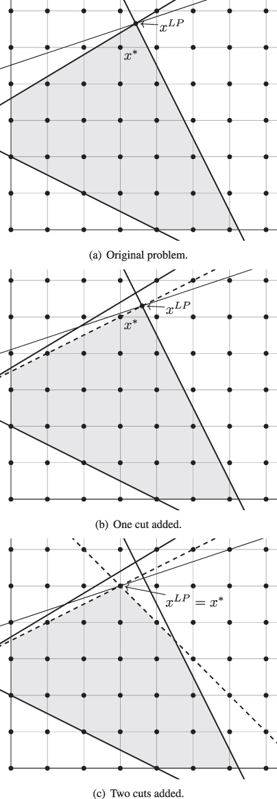
Figure 10.6 Cutting planes.
Now consider the following constraint:
Constraint 10.13 is a cut, because it is satisfied by every feasible integer solution for 10.12 (see the dashed line in Figure 10.6(b)) but not by every feasible solution for the LP relaxation of 10.12. In particular, ![]() violates 10.13. Therefore, adding 10.13 to the problem shrinks the LP feasible region, and thus tightens the LP bound. The new LP solution is
violates 10.13. Therefore, adding 10.13 to the problem shrinks the LP feasible region, and thus tightens the LP bound. The new LP solution is ![]() , with
, with ![]() .
.
Adding the cut 10.13 does not quite reduce the LP feasible region to the convex hull of the IP feasible set near the optimal solution. But adding one more cut will do the trick:
Now we have ![]() . (See Figure 10.6(c).) In other words, solving the LP relaxation is equivalent to solving the IP itself.
. (See Figure 10.6(c).) In other words, solving the LP relaxation is equivalent to solving the IP itself.
This raises the question: How do we identify good cuts, i.e., constraints that “separate” the current LP solution? The problem of finding such a cut is called the separation problem. In most cutting‐plane methods, including those for the TSP, researchers first identify families of cuts—that is, they identify structures of the cuts but not their coefficients—and then develop algorithms to solve the separation problem—that is, to determine coefficients so that the cuts will render the current LP solution infeasible. In some cases, the separation problem can be solved efficiently (in polynomial time) and exactly, while in others it must be solved heuristically. The separation problem is typically solved at each node of the search tree to generate cuts that tighten the LP relaxations. Through a combination of branching and adding cuts, branch‐and‐cut guides the solution to the LP relaxation towardinteger feasibility.
Several families of cuts are used in modern branch‐and‐cut algorithms for the TSP. One family consists of the subtour‐elimination constraints. As we noted in Section 10.2.2, there are too many subtour‐elimination constraints to include all of them explicitly in the formulation. Therefore, we generate violated subtour‐elimination constraints on the fly during the branch‐and‐bound process. The separation problem—i.e., the problem of deciding which constraints to add on the fly—can be solved in polynomial time (Crowder and Padberg, 1980; Padberg and Rinaldi, 1990a). The basic idea is as follows: Suppose we solve the LP relaxation of 10.7–10.10 with 10.9 replaced by the equivalent constraints 10.5, but only some of these constraints included. Let ![]() be the optimal solution. We wish to find constraints 10.5 that are violated by
be the optimal solution. We wish to find constraints 10.5 that are violated by ![]() . The support graph of this solution has node set N and edge set
. The support graph of this solution has node set N and edge set ![]() , with weight
, with weight ![]() on edge
on edge ![]() . There is a violated constraint 10.5 if and only if there is an
. There is a violated constraint 10.5 if and only if there is an ![]() such that the total weight on the edges out of S is less than 2—in other words, if there is a cut in the support graph whose weight is less than 2. Therefore, finding a violated subtour‐elimination constraint is equivalent to solving a minimum‐cut problem, which can be done in polynomial time.
such that the total weight on the edges out of S is less than 2—in other words, if there is a cut in the support graph whose weight is less than 2. Therefore, finding a violated subtour‐elimination constraint is equivalent to solving a minimum‐cut problem, which can be done in polynomial time.
Asecond family of cuts are called 2‐matching inequalities, or Blossom inequalities (Hong, 1972). Suppose we have a set ![]() and s pairwise disjoint sets
and s pairwise disjoint sets ![]() such that each
such that each ![]() contains exactly two nodes, one in H and one not in H, and such that s is odd and at least 3. (See Figure 10.7 for an illustration.) Anticipating the comb inequalities discussed next, H is called the handle and the
contains exactly two nodes, one in H and one not in H, and such that s is odd and at least 3. (See Figure 10.7 for an illustration.) Anticipating the comb inequalities discussed next, H is called the handle and the ![]() are called teeth. A 2‐matching inequality has the form
are called teeth. A 2‐matching inequality has the form

In other words, the number of tour edges contained within the handle plus the number of edges contained within teeth cannot exceed ![]() . The next theorem confirms that 10.15 is a valid inequality for the TSP, i.e., a cut.
. The next theorem confirms that 10.15 is a valid inequality for the TSP, i.e., a cut.

Figure 10.7 Handle and teeth for 2‐matching inequality.
2‐matching inequalities can be written in various other forms. For example, the next proposition gives an equivalent inequality.
The separation problem for 2‐matching inequalities can be solved in polynomial time. Padberg and Rao (1982) provided the first such algorithm, which relies on solving max‐flow problems on a specialized graph. Subsequent improvements to this algorithm were proposed by Grötschel and Holland (1987) and Letchford et al. (2004).
Ifthe teeth are allowed to have more than two nodes each—but at least one node in H and one node not in H—then we have a comb, as depicted in Figure 10.8. Combs give rise to the following comb inequalities:

As with 2‐matching inequalities10.15, the left‐hand side represents the number of edges of the tour that are contained within the handle or within the teeth. Comb inequalities are valid inequalities, as the next theorem attests.

Figure 10.8 Handle and teeth for comb inequality.
Comb inequalities can also be written in other forms; for example, 10.16 is valid for comb inequalities, as well. (See Problem 10.11.)
Grötschel and Padberg (1979) prove that comb inequalities and subtour‐elimination constraints together are facet‐defining, which means that if we add all possible comb inequalities to the feasible region of the LP relaxation of 10.7–10.10, the LP relaxation will equal the convex hull of the IP, and solving the LP relaxation will be equivalent to solving the TSP itself. Unfortunately, there is no known polynomial‐time exact separation algorithm for comb inequalities, nor is it known whether the separation problem is NP‐hard (Applegate et al., 2007). Therefore, the problem is generally solved heuristically; see, e.g., Padberg and Rinaldi (1990b), Grötschel and Holland (1991), and Applegate et al. (1995).
Many other types of cuts have been proposed for the TSP. These include clique‐tree (Grötschel and Pulleyblank, 1986), path (Cornuéjols et al., 1985), star (Fleischmann, 1988), hypohamiltonian (Grötschel, 1980a), chain (Padberg and Hong, 1980), and ladder inequalities (Boyd et al., 1995). See Applegate et al. (2007) for an in‐depth discussion of the branch‐and‐cut approach for the TSP, including a detailed description of how branch‐and‐cut is implemented in the Concorde TSP solver (Applegate et al., 2006), widely recognized as the most powerful exact TSP solver available.
10.4 Construction Heuristics for theTSP
In this section, we discuss construction heuristics for the TSP. For some heuristics, we will prove that, for all instances,
where ![]() is the objective value of the solution returned by a given heuristic H,
is the objective value of the solution returned by a given heuristic H, ![]() is the optimal objective value, and
is the optimal objective value, and ![]() is a constant. Equation 10.21 provides a fixed worst‐case error bound. If a heuristic executes in polynomial time (as most heuristics do, otherwise an exact algorithm may be preferable) and a bound of the form in 10.21 exists, the heuristic is called an approximation algorithm, or sometimes an
is a constant. Equation 10.21 provides a fixed worst‐case error bound. If a heuristic executes in polynomial time (as most heuristics do, otherwise an exact algorithm may be preferable) and a bound of the form in 10.21 exists, the heuristic is called an approximation algorithm, or sometimes an ![]() ‐approximation algorithm.
‐approximation algorithm.
It is nice when such bounds are available, since then we have a guarantee on the performance of the heuristic. Unfortunately, not all heuristics have fixed worst‐case bounds—some heuristics may return solutions that are arbitrarily far from the optimal solution. In fact, the situation is even worse: For general distance matrices (for which the triangle inequality need not hold), there are no polynomial‐time approximation algorithms, unless P = NP (Sahni and Gonzalez, 1976):
Note that the distance matrix in the proof of Theorem 10.5 may not satisfy the triangle inequality. This is an important point, because, as we will see, there are polynomial‐time heuristics that have fixed worst‐case bounds if the triangle inequality holds.
We now discuss several construction heuristics. The heuristics in Sections 10.4.1–10.4.5 are called insertion heuristics because they begin with an empty tour and iteratively insert nodes onto the tour. Much the analysis in those sections derives from Rosenkrantz et al. (1977). The heuristics in Sections 10.4.6 and 10.4.7, in contrast, begin by constructing a minimum spanning tree and then building a tour based on the tree.
10.4.1 Nearest Neighbor
We begin with a very simple heuristic called the nearest neighbor (NN) heuristic. The heuristic begins with an arbitrary node. At each iteration, we add the unvisited node that is closest to the current node (and set that node as the new current node). When all nodes have been added, we return to the starting node. The NN heuristic executes in ![]() time, where n is the number of nodes.
time, where n is the number of nodes.
Algorithm 10.1 lists pseudocode for the NN heuristic. In the pseudocode, ![]() represents the set of nodes that are on the current tour and
represents the set of nodes that are on the current tour and ![]() represents the current node.
represents the current node.

Clearly, the NN heuristic can easily get “boxed into a corner” from which the only escape is an unattractively long edge (such as ![]() in Example 10.2). The NN tour falls into similar traps in the Car 54 instance, as shown in Figure 10.10. It has a total distance of 13,044 miles (compared to the optimal tour's distance of 10,861). Although Rosenkrantz et al. (1977) report good performance of NN on a small computational experiment, subsequent experiments have reported worse performance compared to other insertion methods (Golden and Stewart, 1985).
in Example 10.2). The NN tour falls into similar traps in the Car 54 instance, as shown in Figure 10.10. It has a total distance of 13,044 miles (compared to the optimal tour's distance of 10,861). Although Rosenkrantz et al. (1977) report good performance of NN on a small computational experiment, subsequent experiments have reported worse performance compared to other insertion methods (Golden and Stewart, 1985).
We now examine the theoretical worst‐case behavior of NN.
The first part of Theorem 10.6 seems like good news, since 10.23 seems like the type of bound we try to prove. However, the bound in the right‐hand side of 10.23 is not fixed—it increases with n. Still, this is just an upper bound; maybe the actual ratio doesn't increase with n, leaving open the possibility that some future researcher will prove a fixed worst‐case bound. Alas, the second part of the theorem dashes these hopes by proving that we can find instances with arbitrarily bad performance.

Figure 10.10 Nearest‐neighbor solution to Car 54 TSP instance. Total distance = 13,044 miles.
10.4.2 Nearest Insertion
The nearest insertion (NI) heuristic works as follows: We begin with a tour consisting of an arbitrary node. At each subsequent iteration, we find the unvisited node ![]() that is closest to a node m on the tour; node
that is closest to a node m on the tour; node ![]() will be the next node to insert onto the tour. If the tour only contains one node thus far, we insert
will be the next node to insert onto the tour. If the tour only contains one node thus far, we insert ![]() after it; otherwise, we find the tour edge
after it; otherwise, we find the tour edge ![]() that minimizes the net change in the tour length due to the insertion, defined by
that minimizes the net change in the tour length due to the insertion, defined by
and replace edge ![]() with edges
with edges ![]() and
and ![]() . (Note that m, the closest tour node to
. (Note that m, the closest tour node to ![]() , will not necessarily equal the
, will not necessarily equal the ![]() or
or ![]() that minimize
that minimize ![]() .) We continue in this way until all cities have been inserted onto the tour. The NI heuristic executes in
.) We continue in this way until all cities have been inserted onto the tour. The NI heuristic executes in ![]() time. The heuristic is described in pseudocode in Algorithm 10.2.
time. The heuristic is described in pseudocode in Algorithm 10.2.
The NI tour in Example 10.3 is actually longer than the NN tour in Example 10.2 (even though it looks more reasonable). In general though, NI is a more effective heuristic than NN. For example, the NI tour for the Car 54 instance, shown in Figure 10.12, has a total distance of 12,588 miles, compared to 13,044 for NN (and 10,861 for the optimal tour).

Figure 10.12 Nearest‐insertion solution to Car 54 TSP instance. Total distance = 12,588 miles.
In fact, unlike NN, NI has a fixed worst‐case performance bound:
In practice, the ratio ![]() is, of course, often much smaller than 2. For example, the bound for the Car 54 instance is
is, of course, often much smaller than 2. For example, the bound for the Car 54 instance is ![]() . This raises the question: Is it possible to prove a smaller fixed worst‐case bound on
. This raises the question: Is it possible to prove a smaller fixed worst‐case bound on ![]() that applies to all instances? The answer is “no”; the bound of 2 is tight, as the next proposition demonstrates.
that applies to all instances? The answer is “no”; the bound of 2 is tight, as the next proposition demonstrates.

Figure 10.13 TSP instance for proof that NI bound is tight.
Note that Theorem 10.8 says that no better bound is possible for the NI heuristic. It does not say that no heuristic can possibly obtain a better bound. Indeed, Christofides' heuristic, discussed in Section 10.4.7, has a fixed worst‐case bound of 3/2.
A variant of the NI heuristic, called the cheapest insertion (CI) heuristic, searches over all k not on the tour and all edges ![]() on the tour and chooses the insertion with the smallest
on the tour and chooses the insertion with the smallest ![]() ; see Algorithm 10.3. (In contrast, NI first finds the nearest k to the tour, and then finds the minimum
; see Algorithm 10.3. (In contrast, NI first finds the nearest k to the tour, and then finds the minimum ![]() for that k.) CI has a complexity of
for that k.) CI has a complexity of ![]() , slightly higher than NI's
, slightly higher than NI's ![]() complexity. Like NI, CI has a fixed worst‐case bound of 2, and this bound is tight (Rosenkrantz et al., 1977). The cheapest‐insertion tour for the Car 54 instance is shown in Figure 10.14 and has a total length of 12,748.
complexity. Like NI, CI has a fixed worst‐case bound of 2, and this bound is tight (Rosenkrantz et al., 1977). The cheapest‐insertion tour for the Car 54 instance is shown in Figure 10.14 and has a total length of 12,748.

Figure 10.14 Cheapest‐insertion solution to Car 54 TSP instance. Total distance = 12,748 miles.
10.4.3 Farthest Insertion

Thefarthest insertion (FI) heuristic is the same as the NI heuristic except that we choose the node k not on the tour that is farthest from any node on the tour. We then insert k into the edge ![]() that minimizes
that minimizes ![]() , as in NI. In Algorithm 10.2, we simply replace
, as in NI. In Algorithm 10.2, we simply replace ![]() with
with ![]() in line 6. The heuristic has the same complexity as NI:
in line 6. The heuristic has the same complexity as NI: ![]() .
.
It may seem counterintuitive to choose farthest nodes to insert, since we are aiming for a shortest tour. But remember that we are only choosing the farthest node to insert—we still perform the cheapest insertion of that node. The idea is to sketch out the outline of the tour early in the process, and fill in the details later. We will need to visit every node eventually, and there is nothing inherently bad about choosing the far nodes early on.
It is not known whether FI has a fixed worst‐case bound. The empirical performance of FI tends to be good, however (Rosenkrantz et al., 1977; Golden and Stewart, 1985).
The farthest‐insertion tour for the Car 54 instance, shown in Figure 10.16, has a total distance of 10,998 miles—the best tour of any of our heuristics so far, and only 1.3% worse than the optimal distance of 10,861.
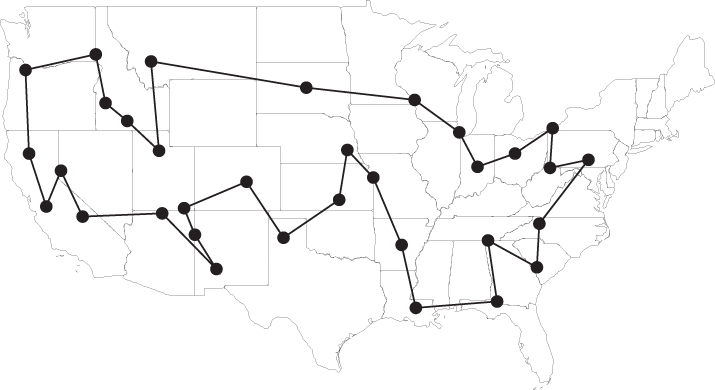
Figure 10.16 Farthest‐insertion solution to Car 54 TSP instance. Total distance = 10,998 miles.
10.4.4 ConvexHull
The convex hull heuristic (Stewart, 1977) generates an initial partial tour by computing the convex hull of the nodes. Then, at each iteration, the heuristic performs the cheapest insertion, i.e., it finds the nontour node k and the tour edge ![]() that minimize
that minimize ![]() , and it inserts k into edge
, and it inserts k into edge ![]() . Like FI, the idea is to generate an outline of the tour quickly and then fill in the remaining nodes. Warburton (1993) proves that the convex hull heuristic has a fixed worst‐case bound of 3 for the Euclidean TSP (i.e., the TSP in which distances are Euclidean), though its performance is usually much better than 3 in practice (Golden and Stewart, 1985).
. Like FI, the idea is to generate an outline of the tour quickly and then fill in the remaining nodes. Warburton (1993) proves that the convex hull heuristic has a fixed worst‐case bound of 3 for the Euclidean TSP (i.e., the TSP in which distances are Euclidean), though its performance is usually much better than 3 in practice (Golden and Stewart, 1985).
The convex hull heuristic returns a tour of length 11,033 for the Car 54 instance; see Figure 10.18.

Figure 10.18 Convex‐hull solution to Car 54 TSP instance. Total distance = 11,033 miles.
Avariant is the greatest angle insertion heuristic (Norback and Love, 1977): We begin with the convex hull, and then choose the nontour k and the tour edge ![]() that maximizes the angle between
that maximizes the angle between ![]() and
and ![]() , and insert k into this edge.
, and insert k into this edge.
10.4.5 GENI
All of the insertion heuristics discussed thus far only allow a node to be inserted into an existing edge of the tour. The generalized insertion (GENI) heuristic by Gendreau et al. (1992) relaxes this requirement, allowing a node to be inserted between any two nodes on the tour.
Suppose we want to insert a node k between nodes i and j on the tour. To do this, we need to remove one of the edges incident to i and one incident to j and replace them with edges to k. This leaves two nodes—the former neighbors of i and j—that have degree 1 and must be reconnected somehow. (See Figure 10.19(a) and (b). The straight lines represent single edges, while the squiggles represent potentially longer portions of the tour.) The obvious fix is to connect the two former neighbors to each other, as in Figure 10.19(c), but this may be a long edge. Or worse, connecting the two former neighbors may result in two subtours rather than one complete tour, as in Figure 10.19(d). The GENI heuristic tries to find more effective (though also more complicated) ways to reconnect the tour after inserting node k.

Figure 10.19 Inserting a node between two nonadjacent nodes in the GENI heuristic.
GENI considers two types of insertions. Type I insertions remove one additional edge, while Type II insertions remove two additional edges, before reconnecting the tour. We'll use subscripts ![]() and
and ![]() to denote the successor and predecessor, respectively, of a given node on the tour under a fixed orientation. For example,
to denote the successor and predecessor, respectively, of a given node on the tour under a fixed orientation. For example, ![]() is the node that comes after i in the tour.
is the node that comes after i in the tour.
Let ![]() be a node on the path from j to i for a particular orientation of the tour, with
be a node on the path from j to i for a particular orientation of the tour, with ![]() . A Type I insertion involves
. A Type I insertion involves
- deleting edges
 ,
,  , and
, and  , and
, and - adding edges
 ,
,  ,
,  , and
, and  .
.
A Type I insertion is depicted in Figure 10.20. In the tour resulting from a Type I insertion, the segments from ![]() to j and from
to j and from ![]() to
to ![]() are reversed, while the segment from
are reversed, while the segment from ![]() to i is unchanged. Note that if
to i is unchanged. Note that if ![]() and
and ![]() , then a Type I insertion is equivalent to the standard insertion—inserting a node between two consecutive nodes.
, then a Type I insertion is equivalent to the standard insertion—inserting a node between two consecutive nodes.

Figure 10.20 GENI Type I insertion.
Let ![]() be a node on the path from j to i and let m be a node on the path from i to j for a particular orientation of the tour, with
be a node on the path from j to i and let m be a node on the path from i to j for a particular orientation of the tour, with ![]() and
and ![]() . A Type II insertion involves
. A Type II insertion involves
- deleting edges
 ,
,  ,
,  , and
, and  , and
, and - adding edges
 ,
,  ,
,  ,
,  , and
, and  .
.
(See Figure 10.21.) Like Type I insertions, Type II insertions result in two tour segments reversing direction, in this case the segments from ![]() to
to ![]() and from m to j.
and from m to j.

Figure 10.21 GENI Type II insertion.
For a given choice of k, there are ![]() choices for
choices for ![]() in a Type I insertion and
in a Type I insertion and ![]() choices for
choices for ![]() in Type II, times two possible tour orientations. This is a lot of combinations to check, so Gendreau et al. (1992) suggest simplifying the search for good insertions by making use of p‐neighborhoods. If node i is on the tour, its p‐neighborhood
in Type II, times two possible tour orientations. This is a lot of combinations to check, so Gendreau et al. (1992) suggest simplifying the search for good insertions by making use of p‐neighborhoods. If node i is on the tour, its p‐neighborhood ![]() is defined as the p nodes on the tour (excluding i itself) that are closest to i as measured by
is defined as the p nodes on the tour (excluding i itself) that are closest to i as measured by ![]() . If the tour has fewer than p nodes in addition to i, then they are all in
. If the tour has fewer than p nodes in addition to i, then they are all in ![]() . For example, in the tour in Figure 10.22,
. For example, in the tour in Figure 10.22, ![]() .
.
The GENI heuristic restricts the possible combinations for Type I and II insertions as follows:
-

-

-
 (for Type II).
This significantly reduces the number of combinations to check, while targeting new edges ![]() and
and ![]() that are short. p is a parameter of the heuristic, chosen by the modeler, and is usually relatively small, say, 5.
that are short. p is a parameter of the heuristic, chosen by the modeler, and is usually relatively small, say, 5.

Figure 10.22 4‐neighborhood of node 5.
When inserting k between consecutive nodes i and j, as in the NI and related heuristics, the total tour length cannot decrease, since ![]() in 10.25 due to the triangle inequality. Interestingly, however, GENI insertions do sometimes result in a shorter total tour. (See Problem 10.7.)
in 10.25 due to the triangle inequality. Interestingly, however, GENI insertions do sometimes result in a shorter total tour. (See Problem 10.7.)
The GENI heuristic is summarized in pseudocode in Algorithm 10.4. The heuristic runs in ![]() time. The heuristic is very effective, especially when combined with the unstringing and stringing (US) improvement heuristic described in Section 10.5.3. GENI insertions have also been incorporated into metaheuristics such as tabu search, variable neighborhood search, and ant colony optimization (Gendreau et al., 1994; Mladenović and Hansen, 1997; Le Louarn et al., 2004).
time. The heuristic is very effective, especially when combined with the unstringing and stringing (US) improvement heuristic described in Section 10.5.3. GENI insertions have also been incorporated into metaheuristics such as tabu search, variable neighborhood search, and ant colony optimization (Gendreau et al., 1994; Mladenović and Hansen, 1997; Le Louarn et al., 2004).

10.4.6 Minimum Spanning Tree Heuristic
The next two heuristics we will discuss begin by finding a minimum spanning tree (MST) on the nodes and then converting it to a TSP tour. They therefore function differently from the heuristics described thus far, which iterate through the nodes, inserting one at a time.
Recall that an MST of a network is a minimum‐cost tree that contains every node of the network. Finding an MST is easy using a greedy approach. Prim's algorithm (Prim, 1957) begins with a single node and, at each iteration, adds the shortest edge that connects a node not on the tree to a node on the tree. Kruskal's algorithm (Kruskal, 1956) begins with an empty tree and, at each iteration, adds the shortest edge (whether or not one of its nodes is contained in the tree) that does not create a cycle. Both algorithms run in ![]() time (where E is the set of edges in the network) when implemented using efficient data structures.
time (where E is the set of edges in the network) when implemented using efficient data structures.
Every TSP tour consists of a spanning tree (in particular, a spanning path) plus one edge. This suggests we can use MSTs to generate TSP tours, and to derive useful lower bounds.
The minimum spanning tree heuristic for the TSP begins by finding an MST using Prim's or Kruskal's algorithm or any other method. Next, it doubles every edge to create a network in which every node has even degree. Such a network is called an Eulerian network and is guaranteed to have an Eulerian tour (a tour that traverses every edge exactly once but may visit each node multiple times):
The Eulerian tour derived from the doubled MST gives us a sequence of nodes (each potentially appearing multiple times), which the heuristic converts to a TSP tour simply by skipping any duplicates—this is called shortcutting.
The MST heuristic is summarized in Algorithm 10.5.

The tour returned by the MST heuristic for the Car 54 instance is shown in Figure 10.24. The tour has length 14,964 miles. Bentley (1992) confirms the relatively poor empirical performance of the MST heuristic.

Figure 10.24 Tour obtained by applying MST heuristic to Car 54 instance. Total distance = 14,964 miles.
The minimum spanning tree heuristic has a fixed worst‐case bound of 2:
This bound is tight; seeProblem 10.12.
10.4.7 Christofides' Heuristic
Like the minimum spanning tree heuristic, Christofides' heuristic (Christofides, 1976) builds an MST and then converts it to a TSP tour. The difference is in the way the heuristics modify the MST to create an Eulerian network. Whereas the minimum spanning tree heuristic simply doubles every edge, Christofides' heuristic takes a more sophisticated, and more effective, approach. By Theorem 10.10, it is the odd‐degree nodes that prevent the MST from having an Eulerian tour. Christofides's heuristic adds a single edge to each of these nodes to produce a graph whose nodes all have even degree. It is possible to pair up the odd‐degree nodes because there are always an even number of them:
(This lemma is called the handshaking lemma: If a set of people shake hands at a party, there must be an even number of people who shook hands with an odd number of people.)
A matching on a set of nodes is a set of edges such that every node is contained in at most one edge. A perfect matching is a set of edges such that every node is contained in exactly one edge. (See Figure 10.25.) Christofides' heuristic finds a minimum‐weight perfect matching on the odd‐degree nodes in the MST, where the weights are given by the edge lengths. A minimum‐weight perfect matching can be found in polynomial time (Edmonds, 1965). The matching may duplicate edges already in the MST. A perfect matching on the odd‐degree nodes must exist, by Lemma 10.12. When the matching edges are added to the MST, every node has even degree (since we are adding a single edge to each odd‐degree node), so the resulting network is Eulerian. The heuristic then finds an Eulerian tour and converts it to a TSP tour by shortcutting, exactly as in the minimum spanning tree heuristic. The heuristic is summarized in Algorithm 10.6.

Figure 10.25 Matchings.
Christofides' heuristic produces an 11,654‐mile tour for the Car 54 instance (Figure 10.27), much better than the 14,964‐mile tour returned by the MST heuristic (Figure 10.24) and approximately 7.3% longer than the optimal tour.

Figure 10.27 Tour obtained by applying Christofides' heuristic to Car 54 instance. Total distance = 11,654 miles.
Christofides' heuristic has the best fixed worst‐case bound known to date.

Figure 10.28 Optimal TSP tour on odd‐degree nodes in MST in Christofides' heuristic, and two perfect matchings (solid and dashed) that constitute it.
The ![]() bound in Theorem 10.13 is tight;see Problem 10.13.
bound in Theorem 10.13 is tight;see Problem 10.13.
10.5 Improvement Heuristics for theTSP
The tours returned by the construction heuristics discussed in Section 10.4 are typically not optimal. In this section, we discuss improvement heuristics for the TSP that begin with a complete tour and perform operations on it to try to make it shorter.
10.5.1 k‐Opt Exchanges
One can tell just by looking at Figure 10.10 that the nearest‐neighbor solution for the Car 54 instance is bad. The most obvious red flag is that the tour crosses itself several times.
Of course, the Car 54 distances are not Euclidean (they come from road networks), but you might still suspect that we can improve the tour in Figure 10.10 by “uncrossing” it. One mechanism for doing this is called a 2‐opt exchange. In a 2‐opt, we remove two edges and replace them with two other edges to form a new tour. For a given pair of edges, there are two possible ways to reconnect the tour, shown in Figure 10.29. However, the replacement edges in Figure 10.29(a) are the same as the original edges that were removed, so the only real option is the strategy in Figure 10.29(b). (Replacing ![]() and
and ![]() with
with ![]() and
and ![]() is also not an option since this creates two subtours rather than one contiguous tour.) The 2‐opt idea was introduced by Flood (1956) (in the very first issue of the journal Operations Research, after it subsumed the Journal of the ORSA) as a way to fix crossing tours generated by his algorithm; shortly thereafter, Croes (1958) developed a construction heuristic with 2‐opt exchanges as the centerpiece.
is also not an option since this creates two subtours rather than one contiguous tour.) The 2‐opt idea was introduced by Flood (1956) (in the very first issue of the journal Operations Research, after it subsumed the Journal of the ORSA) as a way to fix crossing tours generated by his algorithm; shortly thereafter, Croes (1958) developed a construction heuristic with 2‐opt exchanges as the centerpiece.

Figure 10.29 Two possible ways to reconnect tour during 2‐opt exchange.
To describe the 2‐opt exchange more formally, suppose ![]() and
and ![]() are disjoint edges in the tour and that, for a given orientation of the tour, node i comes before j and node k comes before
are disjoint edges in the tour and that, for a given orientation of the tour, node i comes before j and node k comes before ![]() . Then a 2‐opt exchange consists of replacing edges
. Then a 2‐opt exchange consists of replacing edges ![]() and
and ![]() with edges
with edges ![]() and
and ![]() . This also changes the orientation of the
. This also changes the orientation of the ![]() portion of the tour. For Euclidean problems, a given 2‐opt exchange will only reduce the total length of the tour if edges
portion of the tour. For Euclidean problems, a given 2‐opt exchange will only reduce the total length of the tour if edges ![]() and
and ![]() cross each other, since otherwise the new edges
cross each other, since otherwise the new edges ![]() and
and ![]() will cross each other.
will cross each other.
The 2‐opt heuristic iterates through all pairs of edges looking for 2‐opt exchanges that improve the objective function. The procedure terminates when no such pairs can be found. At each iteration, there are ![]() pairs of edges to consider. The heuristic is simple and effective. A single 2‐opt exchange (exchanging edges
pairs of edges to consider. The heuristic is simple and effective. A single 2‐opt exchange (exchanging edges ![]() and
and ![]() for edges
for edges ![]() and
and ![]() ) is sufficient to “fix” the nearest‐neighbor tour for the 8‐node problem in Example 10.2. When applied to the nearest‐neighbor Car 54 solution in Figure 10.10, the 2‐opt heuristic results in the tour shown in Figure 10.30, whose length is 10,944 miles—only 0.76% longer than the optimal tour.
) is sufficient to “fix” the nearest‐neighbor tour for the 8‐node problem in Example 10.2. When applied to the nearest‐neighbor Car 54 solution in Figure 10.10, the 2‐opt heuristic results in the tour shown in Figure 10.30, whose length is 10,944 miles—only 0.76% longer than the optimal tour.

Figure 10.30 Tour obtained by applying 2‐opt heuristic to nearest‐neighbor tour for Car 54 instance. Total distance = 10,944 miles.
Buildingon this idea, we can try removing three edges and replacing them with alternative edges. This is the idea behind the 3‐opt exchange (Lin, 1965). When we remove three disjoint edges, there are eight possible ways to reconnect the tour, as shown in Figure 10.31. The first reconnection in Figure 10.31 is identical to the original tour, but the remaining seven strategies could all potentially result in shorter tours. The 3‐opt method is powerful but also computationally costly: There are ![]() triplets of edges to consider, and for each, we must evaluate seven possible reconnections. (Recall that 2‐opt requires considering
triplets of edges to consider, and for each, we must evaluate seven possible reconnections. (Recall that 2‐opt requires considering ![]() pairs of edges and evaluating one possible reconnection for each.) We could even try general k‐opt exchanges for
pairs of edges and evaluating one possible reconnection for each.) We could even try general k‐opt exchanges for ![]() , but the computational burden makes the search for such exchanges impractical.
, but the computational burden makes the search for such exchanges impractical.

Figure 10.31 Eight possible ways to reconnect tour during 3‐opt exchange.
The search for higher‐order k‐opt exchanges is not hopeless, however. The Lin–Kernighan heuristic (Lin and Kernighan, 1973) finds k‐opt exchanges by aggregating multiple 2‐opt exchanges, allowing some intermediate exchanges that may even increase the tour length so long as the ultimate result is an improvement. Johnson and McGeoch (1997) report computational experiments showing the Lin–Kernighan heuristic to come within 1.5% of the optimal tour, on average, for random instances with up to a million nodes. The heuristic is so powerful that it is a component of nearly every modern exact algorithm for the TSP, even though the heuristic itself is over 35 years old (Applegate et al., 2007). An important enhancement is the chained Lin–Kernighan heuristic by Martin et al. (1991), which contains a feature for the algorithm to “kick” the tour, i.e., to modify it slightly, when the search appears to be stuck. The variant on chained Lin–Kernighan by Johnson (1995) can solve large instances to within 0.1% optimality (Johnson and McGeoch, 1997).
10.5.2 Or‐Opt Exchanges
An Or‐opt exchange (Or, 1976) takes a segment of the tour consisting of p consecutive nodes and moves it to another spot on the tour, possibly reversing the order of the p nodes as well. A few examples with ![]() are shown in Figure 10.32. Typically, p is relatively small; one common implementation searches for exchanges with
are shown in Figure 10.32. Typically, p is relatively small; one common implementation searches for exchanges with ![]() , then repeats for
, then repeats for ![]() , then for
, then for ![]() , and then terminates. Or‐opt can be implemented efficiently, with
, and then terminates. Or‐opt can be implemented efficiently, with ![]() complexity at each iteration.
complexity at each iteration.

Figure 10.32 Or‐opt exchanges.
A single Or‐opt exchange—moving node 3 so that it comes after node 6 rather than node 8 (orienting the tour clockwise)—is sufficient to “fix” the nearest‐neighbor tour in Example 10.2. The iterative approach described above, applied to the Car 54 nearest‐neighbor tour (Figure 10.30), performs one Or‐opt with ![]() , three with
, three with ![]() , and four with
, and four with ![]() . The resulting tour is shown in Figure 10.33 and has a total length of 11,212 miles—not quite as impressive as the 10,944‐mile tour found by 2‐opt, but close. Actually, a few 2‐opt exchanges applied after the Or‐opt procedure would convert the tour to the 10,944‐mile solution. The idea of combining Or‐opt and 2‐opt exchanges is actually quite powerful, with the ability to generate high‐quality tours while being much simpler to code than Lin–Kernighan and other hybrid exchange heuristics (Babin et al., 2007).
. The resulting tour is shown in Figure 10.33 and has a total length of 11,212 miles—not quite as impressive as the 10,944‐mile tour found by 2‐opt, but close. Actually, a few 2‐opt exchanges applied after the Or‐opt procedure would convert the tour to the 10,944‐mile solution. The idea of combining Or‐opt and 2‐opt exchanges is actually quite powerful, with the ability to generate high‐quality tours while being much simpler to code than Lin–Kernighan and other hybrid exchange heuristics (Babin et al., 2007).

Figure 10.33 Tour obtained by applying Or‐opt heuristic to nearest‐neighbor tour for Car 54 instance. Total distance = 11,212 miles.
10.5.3 Unstringing and Stringing
Gendreau et al. (1992) propose an improvement heuristic called unstringing and stringing (US). The idea is to remove a node from the tour and then reinsert it at another spot. (Think of removing a bead from a string and then replacing it elsewhere on the string.) This sounds like an Or‐opt exchange with ![]() , but the difference is that the tour need not simply close up around the removed node, and the insertion need not occur between two consecutive nodes.
, but the difference is that the tour need not simply close up around the removed node, and the insertion need not occur between two consecutive nodes.
In the US heuristic, “stringing” occurs using Type I or Type II GENI insertions (see Section 10.4.5), while “unstringing” is the reverse. In particular, suppose that the path from ![]() to
to ![]() contains nodes called i, j, and
contains nodes called i, j, and ![]() , in that order. (Recall that the superscripts
, in that order. (Recall that the superscripts ![]() and
and ![]() refer to successors and predecessors.) Then a Type I unstringing of node k removes edges
refer to successors and predecessors.) Then a Type I unstringing of node k removes edges ![]() ,
, ![]() ,
, ![]() , and
, and ![]() and replaces them with
and replaces them with ![]() ,
, ![]() , and
, and ![]() ; see Figure 10.34. A Type II unstringing of node k removes edges
; see Figure 10.34. A Type II unstringing of node k removes edges ![]() ,
, ![]() ,
, ![]() ,
, ![]() , and
, and ![]() and replaces them with
and replaces them with ![]() ,
, ![]() ,
, ![]() , and
, and ![]() ; see Figure 10.35. As in the GENI heuristic, we restrict the possible combinations by making use of p‐neighborhoods; see Gendreau et al. (1992) for details.
; see Figure 10.35. As in the GENI heuristic, we restrict the possible combinations by making use of p‐neighborhoods; see Gendreau et al. (1992) for details.

Figure 10.34 US Type I unstringing of node k.

Figure 10.35 US Type II unstringing of node k.
Gendreau et al. (1992) recommend combining the GENI construction heuristic and the US improvement heuristic to obtain—naturally—the GENIUS heuristic. They report favorable computational results for the GENIUS heuristic compared to several others, including 2‐opt and Lin–Kernighan (though on a rather limited set ofinstances).
10.6 Bounds and Approximations for the TSP
Using several heuristics, we have found a tour with total distance 81 for the instance in Figure 10.5. This might suggest that this tour is optimal—but how can we know for sure? If we did not want to or could not solve the instance using an exact method, an alternative is to find a lower bound on the optimal tour length. If the lower bound equals 81, then we know our tour is optimal. If not, then at least we have a benchmark against which to compare our solution.
Theorems 10.1 and 10.11 provide lower bounds on the optimal TSP tour length. For the instance in Figure 10.5, these theorems provide bounds of 79 and 55, respectively. In Sections 10.6.1 and 10.6.2, we discuss two more powerful and flexible lower bounds. We also discuss the related question of bounding the integrality gap, i.e., the gap between the TSP and its LP relaxation, in Section 10.6.3. In Section 10.6.4, we discuss approximation bounds, i.e., bounds on the constant ![]() in 10.21 that can be proven for a polynomial‐time heuristic. Then, in Section 10.6.5, we discuss the asymptotic behavior of the optimal tour length as
in 10.21 that can be proven for a polynomial‐time heuristic. Then, in Section 10.6.5, we discuss the asymptotic behavior of the optimal tour length as ![]() , including the well‐known square‐root approximation for the TSP.
, including the well‐known square‐root approximation for the TSP.
10.6.1 The Held–Karp Bound
FromLemma 10.9, we know that the total length of the edges in an MST is a lower bound on that of the optimal TSP tour. This is an interesting fact, but not usually a particularly strong bound. For example, an MST for the instance in Figure 10.9 has total length 55 (much smaller than our current best solution of 81). Similarly, an MST for the Car 54 instance has total length 9425; it is pictured in Figure 10.36. This bound is 13.2% smaller than the optimal tour length of 10,861.

Figure 10.36 Minimum spanning tree for Car 54 instance. Total distance = 9425 miles.
Oneobvious problem with the MST bound is that a spanning tree only has ![]() edges, whereas a TSP tour has n. This suggests we can improve the bound by adding another edge, and indeed, this is the idea behind one of the most important lower bounds that have been developed, called the Held–Karp bound (Held and Karp, 1970). The bound is derived from a construct that Held and Karp call a 1‐tree, defined as a spanning tree on nodes
edges, whereas a TSP tour has n. This suggests we can improve the bound by adding another edge, and indeed, this is the idea behind one of the most important lower bounds that have been developed, called the Held–Karp bound (Held and Karp, 1970). The bound is derived from a construct that Held and Karp call a 1‐tree, defined as a spanning tree on nodes ![]() plus two edges incident to node 1.
2
plus two edges incident to node 1.
2
Every TSP tour is a 1‐tree, and therefore the problem of finding the minimum‐weight 1‐tree is a relaxation of the TSP.
Moreover, it is easy to find an optimal 1‐tree for a given instance: We simply find an MST on ![]() and then add the two shortest edges connecting node 1 to the MST. Figure 10.37(a) shows the optimal 1‐tree for the Car 54 instance. It has a total length of 9866 miles, providing a better bound on the optimal TSP tour than the MST. We can get even tighter bounds by building optimal 1‐trees rooted at each node (that is, labeling each node “node 1”) in turn; the longest such 1‐tree is rooted at Manuelito, TX and has a total distance of 10,007 miles (Figure 10.37(b)).
and then add the two shortest edges connecting node 1 to the MST. Figure 10.37(a) shows the optimal 1‐tree for the Car 54 instance. It has a total length of 9866 miles, providing a better bound on the optimal TSP tour than the MST. We can get even tighter bounds by building optimal 1‐trees rooted at each node (that is, labeling each node “node 1”) in turn; the longest such 1‐tree is rooted at Manuelito, TX and has a total distance of 10,007 miles (Figure 10.37(b)).

Figure 10.37 Optimal 1‐trees for Car 54 instance.
But we can do even better. To see how, consider the network in Figure 10.38(a). The labels on the edges indicate their lengths. Edges that are not included in the figure are assumed to have a distance of ![]() . The optimal TSP length is 20 units, for example, for the tour
. The optimal TSP length is 20 units, for example, for the tour ![]() . An optimal 1‐tree on this network, shown in Figure 10.38(b), has a total length of 10. So far, this is not too impressive a bound.
. An optimal 1‐tree on this network, shown in Figure 10.38(b), has a total length of 10. So far, this is not too impressive a bound.

Figure 10.38 1‐tree example.
Now suppose we increase the lengths of all edges incident to node 4 by 10 units (Figure 10.38(c)). This increases the length of any TSP tour by exactly 20 units, since every TSP tour traverses exactly two of these edges. Therefore, the optimal TSP tour doesn't change, though its length does, to 40 units. The optimal 1‐tree, shown in Figure 10.38(d), now has length 40. By Lemma 10.15, 40 is a lower bound on the optimal TSP tour for the revised network, and since we have a tour of length 40, that tour must be optimal. Moreover, since the optimal tour for the revised network is also optimal for the original network, the 1‐tree on the revised network provides us a guarantee that our original TSP tour is optimal.
This idea becomes even more powerful when we add weights (constants) to the edges incident to multiple nodes—possibly all of them. Suppose we add a weight of ![]() to all of the edges incident to node i. (We'll usually just say “add a weight of
to all of the edges incident to node i. (We'll usually just say “add a weight of ![]() to node i.”) Let
to node i.”) Let ![]() be the vector of weights. This gives us a revised distance matrix
be the vector of weights. This gives us a revised distance matrix ![]() :
:
We'll use ![]() and
and ![]() to refer to total distances under the original and revised distance matrices, respectively.
to refer to total distances under the original and revised distance matrices, respectively.
On the other hand, changing the distance matrix can change not only the weight of the optimal 1‐tree but also the structure of the 1‐tree itself. As the weights ![]() change, the length of the optimal TSP tour changes in sync, but the length of the optimal 1‐tree may “jump,” providing better bounds.
change, the length of the optimal TSP tour changes in sync, but the length of the optimal 1‐tree may “jump,” providing better bounds.
The right‐hand side of 10.33 is the Held–Karp lower bound and is denoted ![]() . This bound holds for any
. This bound holds for any ![]() ; now the question is how to find good values of
; now the question is how to find good values of ![]() so that the bound is as tight as possible. Held and Karp (1971) propose using subgradient optimization to improve
so that the bound is as tight as possible. Held and Karp (1971) propose using subgradient optimization to improve ![]() . We start with an arbitrary vector
. We start with an arbitrary vector ![]() , and at each iteration t, after calculating the lower bound, we update
, and at each iteration t, after calculating the lower bound, we update ![]() as follows:
as follows:
where
![]() is the degree of node i in the 1‐tree found during iteration t (i.e., the optimal 1‐tree for weights
is the degree of node i in the 1‐tree found during iteration t (i.e., the optimal 1‐tree for weights ![]() ), and
), and ![]() is the best upper bound found so far. As usual,
is the best upper bound found so far. As usual, ![]() is a constant that is halved when a given number of consecutive iterations passes without improving the lower bound (see page 673).
is a constant that is halved when a given number of consecutive iterations passes without improving the lower bound (see page 673).
A set of weights ![]() tends to provide a better bound if the resulting 1‐tree “looks like” a TSP tour, i.e., its nodes mostly have degree 2. (Why?) One way to think about the update step 10.34–10.35 is that nodes that have degree 1 receive lower weights in the next iteration (encouraging more edges to be incident to them in the next 1‐tree) and nodes that have degree greater than 2 receive higher weights (encouraging fewer edges).
tends to provide a better bound if the resulting 1‐tree “looks like” a TSP tour, i.e., its nodes mostly have degree 2. (Why?) One way to think about the update step 10.34–10.35 is that nodes that have degree 1 receive lower weights in the next iteration (encouraging more edges to be incident to them in the next 1‐tree) and nodes that have degree greater than 2 receive higher weights (encouraging fewer edges).
How tight can the bound be? Held and Karp prove that if we could find the optimal ![]() , the resulting bound would equal the LP relaxation bound:
, the resulting bound would equal the LP relaxation bound:
(For this reason, the name “Held–Karp lower bound” is often used to refer to the LP relaxation bound itself.) In practice we can't usually find the optimal ![]() , but we can find good enough
, but we can find good enough ![]() that the Held–Karp bound is very close to the LP bound—within 0.01% in computational experiments by Johnson and McGeoch (1997).
that the Held–Karp bound is very close to the LP bound—within 0.01% in computational experiments by Johnson and McGeoch (1997).
If all of this is starting to feel a lot like Lagrangian relaxation, you're not wrong. Held and Karp (1970) show that their lower bound is equivalent to the Lagrangian relaxation bound obtained from the formulation 10.7–10.10. The constraints in the Lagrangian subproblem define a polyhedron whose vertices are the set of all 1‐trees. The subproblem therefore has the integrality property, which explains 10.36. Held and Karp (1971) propose subgradient optimization to update the multipliers and show how to embed this approach into a branch‐and‐bound scheme to find feasible—often optimal—solutions in addition to the lower bounds. (See also Balas and Toth (1985).)
In Example 10.8, the 1‐tree problem gave a feasible solution to the TSP, even though it is a relaxation. This does not happen for every instance, but it is not uncommon. For example, for the Car 54 instance, a few hundred iterations of the subgradient optimization procedure described above yield a vector ![]() whose optimal 1‐tree is the optimal TSP tour in Figure 10.3, withlength 10,861.
whose optimal 1‐tree is the optimal TSP tour in Figure 10.3, withlength 10,861.
10.6.2 Control Zones
Supposethe nodes in N are located on the plane and ![]() is the Euclidean distance between nodes i and j—this is the Euclidean TSP. Imagine drawing a disk centered at each node in N so that the disks do not overlap (Figure 10.41(a)). Any tour must enter and exit disk j on its way to and from node j, for every
is the Euclidean distance between nodes i and j—this is the Euclidean TSP. Imagine drawing a disk centered at each node in N so that the disks do not overlap (Figure 10.41(a)). Any tour must enter and exit disk j on its way to and from node j, for every ![]() . This means that the length of any tour must be at least
. This means that the length of any tour must be at least ![]() , where
, where ![]() is the radius of disk j. These disks—called control zones—therefore provide a lower bound on the length of the optimal TSP tour.
is the radius of disk j. These disks—called control zones—therefore provide a lower bound on the length of the optimal TSP tour.
In Figure 10.41(a), we have ![]() . This is not the only possible “packing” of control zones around these nodes, and other packings may produce tighter bounds. For example, the control zones in Figure 10.41(b) have
. This is not the only possible “packing” of control zones around these nodes, and other packings may produce tighter bounds. For example, the control zones in Figure 10.41(b) have ![]() , close to the optimal tour length of 15.7. This gives rise to an optimization problem: We wish to choose radii for the control zones to maximize twice their sum, while ensuring that no two control zones overlap:
, close to the optimal tour length of 15.7. This gives rise to an optimization problem: We wish to choose radii for the control zones to maximize twice their sum, while ensuring that no two control zones overlap:
This optimization problem turns out to be the dual of the LP relaxation of the 2‐matching relaxation; that is, if we remove the subtour‐elimination constraints from 10.7–10.10, allow the ![]() to be fractional, and then take the dual, we will get 10.37–10.38.
to be fractional, and then take the dual, we will get 10.37–10.38.

Figure 10.41 Control zones.
We can't hope for the optimal control‐zone bound to be particularly good, given that it is two levels of relaxation away from the original TSP. But we can improve it significantly. Consider the nodes in Figure 10.42(a). The control zones cannot be enlarged further without overlapping. Any feasible tour must pass through the gap in between the two clusters, but the control‐zone bound will not account for this distance. However, we can draw bands around the clusters, called moats, such that the bands from two different clusters do not overlap. (See Figure 10.42(b).) Any tour must pass through every moat twice, once when approaching the cluster and once when departing it, so we can add twice the sum of the moat widths to the lower bound. This helps a great deal, resulting in lower bounds that are often quite tight (Applegate et al., 2007). In effect, adding moats eliminates subtours, bringing the 2‐matching relaxation closer to the original TSP and the control‐zone bound closer to the optimal TSP value.

Figure 10.42 Moats.
The use of control zones and moats was proposed by Jünger and Pulleyblank (1993). In addition to providing useful lower bounds, control zones also make for beautiful pictures when rendered in color—see especially the Concorde iOS app (Cook, 2018b) and the GEODUAL softwareby Jünger et al. (2009).
10.6.3 IntegralityGap
From Theorem 10.13, we know that
where ![]() is the length of the tour returned by Christofides' heuristic. It turns out that this is true even if we replace the discrete problem 10.7–10.10 with its LP relaxation (Wolsey, 1980; Shmoys and Williamson, 1990), that is:
is the length of the tour returned by Christofides' heuristic. It turns out that this is true even if we replace the discrete problem 10.7–10.10 with its LP relaxation (Wolsey, 1980; Shmoys and Williamson, 1990), that is:
Since ![]() , this gives a fixed worst‐case bound on the integrality gap, defined as the ratio between the IP value and the LP relaxation value.
, this gives a fixed worst‐case bound on the integrality gap, defined as the ratio between the IP value and the LP relaxation value.
Thisbound is not believed to be tight, however. In fact, there are no known instances whose integrality gap exceeds ![]() . This has given rise to the “
. This has given rise to the “![]() conjecture” (e.g., Goemans (1995)):
conjecture” (e.g., Goemans (1995)):
Benoit and Boyd (2008) prove that the ![]() conjecture holds for all networks with up to 10 nodes. Moreover, they give a family of instances for which
conjecture holds for all networks with up to 10 nodes. Moreover, they give a family of instances for which ![]() approaches
approaches ![]() asymptotically as the number of nodes increases, which means that no smaller bound than
asymptotically as the number of nodes increases, which means that no smaller bound than ![]() is possible. Boyd and Elliott‐Magwood (2010) extend this result to networks with up to12 nodes.
is possible. Boyd and Elliott‐Magwood (2010) extend this result to networks with up to12 nodes.
Recall that the 2‐matching relaxation is the formulation 10.7–10.10 without the subtour‐elimination constraints 10.9 (Section 10.3.3). Like the LP relaxation, the 2‐matching relaxation provides a lower bound on the optimal TSP length. Boyd and Carr (1999) prove that the ratio between ![]() (the optimal objective value of the 2‐matching relaxation) and
(the optimal objective value of the 2‐matching relaxation) and ![]() is no more than
is no more than ![]() . Boyd and Carr (2011) conjecture that this ratio is in fact
. Boyd and Carr (2011) conjecture that this ratio is in fact ![]() , and Schalekamp et al. (2014) prove their conjecture, i.e.,that
, and Schalekamp et al. (2014) prove their conjecture, i.e.,that
10.6.4 ApproximationBounds
From Theorem 10.13, we know that it is possible to find a polynomial‐time heuristic with a fixed worst‐case bound of ![]() (i.e., a
(i.e., a ![]() ‐approximation algorithm) for the metric TSP. But it is not known whether a better heuristic, with a better bound, is possible. Since the metric TSP is NP‐hard (Papadimitriou, 1977), no approximation algorithm can achieve a bound of 1 (unless P = NP), and in fact it is known that no approximation algorithm can reduce the bound to
‐approximation algorithm) for the metric TSP. But it is not known whether a better heuristic, with a better bound, is possible. Since the metric TSP is NP‐hard (Papadimitriou, 1977), no approximation algorithm can achieve a bound of 1 (unless P = NP), and in fact it is known that no approximation algorithm can reduce the bound to ![]() (Karpinski et al., 2013) (unless P = NP). Whether the best theoretical bound for an approximation algorithm is
(Karpinski et al., 2013) (unless P = NP). Whether the best theoretical bound for an approximation algorithm is ![]() or
or ![]() or somewhere in between remains an open question.
or somewhere in between remains an open question.
If the ![]() equal Euclidean distances—the Euclidean TSP—then we can get arbitrarily close to 1 in polynomial time. Arora (1998) showed that the Euclidean TSP has a polynomial‐time approximation scheme (PTAS)—a family of polynomial‐time algorithms that, for any
equal Euclidean distances—the Euclidean TSP—then we can get arbitrarily close to 1 in polynomial time. Arora (1998) showed that the Euclidean TSP has a polynomial‐time approximation scheme (PTAS)—a family of polynomial‐time algorithms that, for any ![]() , can approximate the problem to within
, can approximate the problem to within ![]() . For fixed
. For fixed ![]() , the algorithm must be polynomial, though the complexity can be different for different
, the algorithm must be polynomial, though the complexity can be different for different ![]() . Arora's PTAS for the Euclidean TSP runs in
. Arora's PTAS for the Euclidean TSP runs in ![]() time. So, for example, to achieve a worst‐case bound of
time. So, for example, to achieve a worst‐case bound of ![]() , the run time would increase roughly as
, the run time would increase roughly as ![]() —still polynomial, but slow. The PTAS is therefore of more theoretical than practical interest.
—still polynomial, but slow. The PTAS is therefore of more theoretical than practical interest.
Interestingly, even though the Euclidean TSP is a special case of the metric TSP, the metric TSP does not have a PTAS unless P = NP (Arora et al., 1998).
10.6.5 Tour Length as a Function of n
A common rule of thumb is that the optimal length of a TSP tour through n random points is proportional to ![]() (as n gets large). Obviously, the constant of proportionality depends on the size of the region in which the points are located. If the points are located in the unit square, then the constant of proportionality is denoted
(as n gets large). Obviously, the constant of proportionality depends on the size of the region in which the points are located. If the points are located in the unit square, then the constant of proportionality is denoted ![]() and called the TSP constant. This result was formalized in a famous result by Beardwood et al. (1959):
and called the TSP constant. This result was formalized in a famous result by Beardwood et al. (1959):
If the nodes are located in a general region with area A, then 10.41 becomes
No one knows the value of ![]() , but Cook (2012) reports on an ongoing experiment in which he and his colleagues have solved over 600 million randomly generated Euclidean TSP instances and used the results to estimate that
, but Cook (2012) reports on an ongoing experiment in which he and his colleagues have solved over 600 million randomly generated Euclidean TSP instances and used the results to estimate that ![]() .
.
Haimovich and Rinnooy Kan (1985) prove that if the nodes in N are contained in a planar region with area A and perimeter p, then the following upper bound holds on ![]() :
:
This bound is not particularly tight. If the region is the unit square, for example, then the right‐hand side of 10.43 is ![]() , which is much larger than the estimate
, which is much larger than the estimate ![]() from Theorem 10.12.
from Theorem 10.12.
10.7 World Records
In addition to sparking creativity and dedication among researchers, the TSP has also ignited their competitive spirit. A quest to solve larger and larger TSP instances has been ongoing for decades. To count as “solved,” an instance must have both a solution and a proof of optimality—that is, both a feasible solution and a lower bound with equal value.
A reasonable start date for this friendly competition is 1954, when Dantzig et al. (1954) solved a 49‐node instance consisting of one city from each of the United States (at the time, there were only 48) plus Washington, DC. Their solution has a total length of (coincidentally) 12,345 miles. They solved the problem by first eliminating seven consecutive cities from the east coast (since an optimal tour through these cities is easy) and then using a manual cutting‐plane method to solve the remaining 42‐node instance. Their 42‐node solution is pictured in Figure 10.43(a).
New records were established gradually over the subsequent decades. Held and Karp (1971) solved a 64‐node random instance using the method described in Section 10.6.1. Camerini et al. (1975) solved a 67‐node random instance. In 1977, Grötschel solved an instance consisting of 120 German cities using branch‐and‐cut (reprinted as Grötschel (1980b)); see Figure 10.43(c). Lin and Kernighan (1973) solved a 318‐node instance derived from a drilling application using their heuristic, discussed in Section 10.5.1; Padberg and Rinaldi (1987) used branch‐and‐cut to solve an instance consisting of 532 AT&T switches in the United States (Figure 10.43(b)); and in 1987, Grötschel and Holland solved a 666‐node instance consisting of locations in the United States (published in Holland, 1987; Grötschel and Holland, 1991), again using branch‐and‐cut. Another major breakthrough occurred in 1987, when Padberg and Rinaldi announced the solution of a 2392‐node instance arising from printed circuit board drilling (published in Padberg and Rinaldi, 1991); see Figure 10.43(d). They accomplished this using emerging supercomputing resources as well as new cutting planes.
The Concorde solver by Applegate et al. (2006) set and shattered a number of records in the late 1990s and early 2000s. The solver's first major milestone was the solution of a 13,509‐node United States data set in 1998, using 4.1 years of CPU time in a parallel computing environment. Concorde's developers announced the solution of a 15,112‐city German instance (requiring 22.6 CPU years on 110 processors) in 2001 and a 24,978‐node Swedish instance (84.8 CPU years) in 2004. Concorde solved an 85,900‐node instance based on very‐large‐scale integration (VLSI) design in 2006 (136 CPU years), and this is the current world record, as of this book's printing. This instance had been nearly solved for 15 years: A solution of length 142,514,146 was found in 1991; another of length 142,382,641 (0.09% shorter) was found in 2004; and that solution was proved optimal in 2006.
Several large instances remain unsolved. A 100,000‐node instance representing a discretization of the Mona Lisa has, at the time of this printing, a known solution of length 5,757,191 and a lower bound of 5,757,084, for a 0.0019% optimality gap. A 115,475‐node instance consisting of all US cities has a current best known solution of 6,204,999 miles. And the massive “World TSP” data set consisting of all populated cities or towns in the world (plus a few research bases in Antarctica), has 1,904,711 nodes. The current best solution for this instance, from March 2018, has length 7,515,772,107, and the best known lower bound is 7,512,218,268, for a 0.0473% optimality gap.
See Cook (2012,2018a) for much more about TSP world records.

Figure 10.43 TSP world records.
PROBLEMS
- 10.1 (TSP Construction Heuristics #1) Use each of the construction heuristics listed below to find solutions for the network shown in Figure 10.45. Begin the insertion heuristics at node 1.
In the figure, edges that are not pictured have lengths given by shortest‐path distances. The optimal tour on this network is
 , with total length 47. For each heuristic, report the tour found and its length. For heuristics for which worst‐case error bounds are available, confirm that the ratio of the length of the tour returned by the heuristic and the length of the optimal tour is no greater than the bound.
- Nearest neighbor
- Nearest insertion
- Cheapest insertion
- Farthest insertion
- Minimum spanningtree
- Christofides

Figure 10.45 TSP instance for Problems 10.1 and 10.2. Edges that are not pictured have lengths given by shortest‐path distances.
- 10.2 (TSP Improvement Heuristics #1) Consider the following tour on the network given in Figure 10.45:
 . Perform two iterations of each of the improvement heuristics listed below (starting from the original tour for each heuristic). Each iteration consists of one move that improves the solution, but it need not be the optimal such move. Indicate the nodes and/or edges involved in each move, as well as the tour that results and its cost.
- 2‐opt
- 3‐opt
- Or‐opt

Figure 10.46 TSP instance for Problems 10.3 and 10.4. Edges that are not pictured have lengths given by shortest‐path distances.
- 10.3 (TSP Construction Heuristics #2) Repeat Problem 10.1 using the network given in Figure 10.46. Edges that are not pictured have lengths given by shortest‐path distances. The optimal tour on this network is
 , with total length 395.
 - 10.4 (TSP Improvement Heuristics #2) Repeat Problem 10.2 to improve the following tour for the network given in Figure 10.46:
 .
. 
Figure 10.47 TSP instance for Problems 10.5 and 10.6. Distances are Euclidean.
Table 10.1 Node coordinates for Problems 10.5 and 10.6.
i 

i 

1 8.1 1.6 6 1.0 1.4 2 8.9 9.7 7 2.8 4.2 3 1.3 9.6 8 5.5 9.2 4 9.1 4.9 9 9.6 7.9 5 6.3 8.0 10 9.6 9.2 - 10.5 (TSP Construction Heuristics #3) Repeat Problem 10.1 using the network given in Figure 10.47. Coordinates for the nodes in the figure are given in Table 10.1. Distances between nodes are Euclidean. The optimal tour on this network is
 , with total length 33.45.
 - 10.6 (TSP Improvement Heuristics #3) Repeat Problem 10.2 to improve the following tour for the network given in Figure 10.47:
 . Coordinates for the nodes in the figure are given in Table 10.1. Distances between nodes are Euclidean.
 - 10.7 (GENI Insertion Can Shorten Tour) Construct a small example that demonstrates that a GENI insertion can decrease the tour length.
- 10.8 (Proof of Handshaking Lemma) ProveLemma 10.12.
- 10.9 (Proof that Euclidean Tours Do Not Cross Themselves) Prove Lemma 10.14.
- 10.10 (Proof of Comb‐Inequality Theorem) Prove Theorem 10.4.
- 10.11 (Proof of Alternate Comb Inequality) Prove that the alternate 2‐matching inequality 10.16 also holds for combs as defined in Theorem 10.4.
- 10.12 (MST Heuristic Bound is Tight) Prove that the bound of 2 for the MST heuristic in Theorem 10.11 is tight.
- 10.13 (Christofides' Heuristic Bound is Tight) Prove that the bound of
 for Christofides' heuristic in Theorem 10.13 is tight.
 - 10.14 (Proof that P = NP?) What is the logical flaw in the following argument?
For any distance matrix c that does not satisfy the triangle inequality, we can always add a sufficiently large constant M to every element in the matrix so that the new matrix,
 , does satisfy the triangle inequality. Moreover, a tour
  is shorter than
  under c if and only if it is shorter under
  . Apply Christofides' heuristic on the revised instance
  ; then the resulting solution is no more than
  worse than optimal, by Theorem 10.13. Since this works for any TSP instance, even those that do not satisfy the triangle inequality, by Theorem 10.5, P = NP.
 - 10.15 (Proof of Lemma 10.16) ProveLemma 10.16.
- 10.16 (Held–Karp Bound #1) Consider the network in Figure 10.48. Edges that are not pictured have a length of
 .
.- What is the optimal TSP tour on this network, and what is its total length,
 ? What is the optimal 1‐tree
 on this network (“rooted” at node 1), and what is its total length,
  ?
? - Find the best Held–Karp lower bound you can. That is, find weights to add to one or more nodes so that
 and the right‐hand side of 10.33 are as close as possible.

Figure 10.48 TSP instance for Problem 10.16. Edges that are not pictured have a length of
 .
. - What is the optimal TSP tour on this network, and what is its total length,
- 10.17 (Held–Karp Bound #2) Repeat Problem 10.16 for the network in Figure 10.49.

Figure 10.49 TSP instance for Problem 10.17. Edges that are not pictured have a length of
 .
. - 10.18 (TSP with Required Edges) Consider a version of the TSP in which we are given a set M of edges that must be part of the tour. Assume that M is a matching.
- Modify Christofides' heuristic to solve this problem.
- Show that the performance of your heuristic from part (a) has a fixed worst‐case bound of
 .
.
- 10.19 (Equivalence of Subtour‐Elimination Constraints) Prove that 10.5 and 10.6 are equivalent.
- 10.20 (Miller–Tucker–Zemlin Subtour‐Elimination Constraints) Miller et al. (1960)propose introducing new decision variables
 (
( ) for the TSP and then replacing the subtour‐elimination constraints 10.9 with
Prove that the resulting formulation is valid, i.e., that 10.44–10.45 prohibit subtours. (These constraints are called the Miller–Tucker–Zemlin, or MTZ, subtour‐elimination constraints.)
- 10.21 (Stengthened MTZ Constraints) Prove that 10.44 can be replaced with the tighter constraint (10.46)

in the MTZ subtour‐elimination constraints (see Problem 10.20).
- 10.22 (Sequence of Convex Hull Nodes) Let
 be the set of nodes that lie on the convex hull of N in an instance of the Euclidean TSP. Prove that every optimal tour visits the nodes in
  in the same sequence in which they occur on the convex hull.
 - 10.23 (Estimating
 ) Perform a computational experiment to estimate the TSP constant
 from Theorem 10.12 by generating random Euclidean TSP instances on the unit square, solving them optimally, and calculating the ratio between the optimal tour length and
  , where n is the number of nodes.
 - 10.24 (Nearest Neighbor for Asymmetric TSP) Provethat, for the asymmetric TSP (in which the distance matrix need not be symmetric) in which the triangle inequality holds, the nearest neighbor heuristic can produce solutions for which

where n is the number of nodes.
- 10.25 (TSP with Pickup and Delivery) Consider the following variant of the TSP. We must visit a set S of source nodes and a set D of destination nodes, with
 , transporting a single type of item from the source nodes to the destination nodes. Any source node can supply any destination node. Each source unit has 1 unit of supply, each destination node demands 1 unit, and the vehicle has a capacity of 1 unit. Adapt the cheapest insertion heuristic to solve this problem. Explain your heuristic in words as well as in pseudocode.
 - 10.26 (Prize‐Collecting TSP) In the prize‐collecting TSP, there is no constraint requiring every node to be on the tour, but there is a reward
 for visiting node i. The objective is to minimize the total tour length minus the total rewards for nodes visited.
- Formulate the prize‐collecting TSP as a linear integer programming problem.
- Propose a construction heuristic for the prize‐collecting TSP. Explain your heuristic in words as well as in pseudocode.
- 10.27 (1‐Tree Formulation is a Relaxation) The problem of finding an optimal 1‐tree can be formulated as follows: (10.47)
 (10.48)
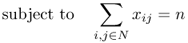 (10.49)
 (10.50)
 (10.51)
Prove that this formulation is a relaxation of the TSP formulation 10.7–10.10.
- 10.28 (Subtour‐Elimination Constraints for
 ) Prove that it is sufficient to replace the “for all” part of constraints 10.9 with
  .
. - 10.29 (Pseudocode for GENI Insertion) Write pseudocode for the procedure to find the best Type I GENI insertion; that is, to implement step 5 in Algorithm 10.4 for Type I insertions.
- 10.30 (Pseudocode for Greedy Heuristic) Thegreedy heuristic for the TSP works as follows: Initialize the tour with the edge
 that minimizes
  . At each subsequent iteration, add to the tour the shortest edge that is not on the tour, does not create a subtour, and does not create a degree‐3 node. (See, e.g., Ong and Moore (1984).) Write pseudocode for this heuristic.
 - 10.31 (Removing Cities from TSP) Suppose we solve the TSP on an arbitrary instance (which satisfies the triangle inequality but is not necessarily Euclidean) and get the optimal tour. Now we decide we do not need to visit one of the cities. Prove or disprove the following claim: The sequence of nodes on the original optimal tour remains optimal after we remove a city; that is, we can simply “close up” the tour around the city we removed.
- 10.32 (Optimal Control Zones) Findthe optimal control zones for the TSP instance in Figure 10.50. The nodes are located at integer coordinates, and the distances among them are Euclidean. Report the radii of each of the control zones, and their sum.

Figure 10.50 TSP instance for Problem 10.32. Distances are Euclidean.