Chapter 5
Stochastic Inventory Models: Continuous
Review
5.1  Policies
In this chapter, we consider a setting similar to the economic order quantity (EOQ)
model (Section 3.2) but with stochastic demand. The mean demand per year is ![]() . The inventory position
is monitored continuously, and orders may be placed at any time. There is a deterministic lead time
L (
. The inventory position
is monitored continuously, and orders may be placed at any time. There is a deterministic lead time
L (![]() ). Unmet demands are
backordered.
). Unmet demands are
backordered.
If the demand has a continuous distribution,
then the inventory level
decreases smoothly but randomly over time, with rate ![]() , as in Figure 5.1. (Think of liquid draining out of a tank at a fluctuating rate.) This is the interpretation used in most of this chapter. Or demands may occur at discrete points in time (as customers arrive), for example, if the demand follows a Poisson process,
as in Section 5.5.
, as in Figure 5.1. (Think of liquid draining out of a tank at a fluctuating rate.) This is the interpretation used in most of this chapter. Or demands may occur at discrete points in time (as customers arrive), for example, if the demand follows a Poisson process,
as in Section 5.5.

Figure 5.1
Inventory level (solid line) and inventory position (dashed line) under  policy.
We'll assume the firm follows an ![]() policy: When the inventory position
reaches a certain point (call it r), we place an order of size Q. L years later, the order arrives. In the intervening time, the inventory on hand may have been sufficient to meet demand, or we may have stocked out. Note that the inventory level
(solid line in Figure 5.1) and inventory position (dashed line)
differ from each other during lead times but coincide otherwise. An
policy: When the inventory position
reaches a certain point (call it r), we place an order of size Q. L years later, the order arrives. In the intervening time, the inventory on hand may have been sufficient to meet demand, or we may have stocked out. Note that the inventory level
(solid line in Figure 5.1) and inventory position (dashed line)
differ from each other during lead times but coincide otherwise. An ![]() policy is known to be optimal for the setting described here, although we will not prove this.
policy is known to be optimal for the setting described here, although we will not prove this.
Whereas the EOQ model has a single decision variable Q, an ![]() policy has two decision variables: Q (the order quantity
, sometimes called the batch size
) and r (the reorder point)
. Our goal is to determine the optimal r and Q to minimize the expected cost per year.
policy has two decision variables: Q (the order quantity
, sometimes called the batch size
) and r (the reorder point)
. Our goal is to determine the optimal r and Q to minimize the expected cost per year.
In
a continuous‐review setting, ![]() policies are equivalent to
policies are equivalent to ![]() policies (Section 4.4) as long as the inventory position equals s exactly at some point in every inventory cycle. This is guaranteed for continuous demand distributions
(as in Sections 5.2–5.4) and for discrete demands in which each customer demands a single unit (as in Section 5.5). Recall that in an
policies (Section 4.4) as long as the inventory position equals s exactly at some point in every inventory cycle. This is guaranteed for continuous demand distributions
(as in Sections 5.2–5.4) and for discrete demands in which each customer demands a single unit (as in Section 5.5). Recall that in an ![]() policy, when the inventory position reaches s, we order up to S. Therefore, a given
policy, when the inventory position reaches s, we order up to S. Therefore, a given ![]() policy is equivalent to an
policy is equivalent to an ![]() policy in which
policy in which ![]() and
and ![]() . On the other hand, this equivalence does not hold for “lumpy” demand processes such as compound Poisson
or for periodic‐review systems,
since in either case the inventory position may fall strictly below the reorder point
before a replenishment order
is placed.
. On the other hand, this equivalence does not hold for “lumpy” demand processes such as compound Poisson
or for periodic‐review systems,
since in either case the inventory position may fall strictly below the reorder point
before a replenishment order
is placed.
In this chapter, we will focus first on the case in which the demands have a continuous distribution . We will discuss an exact model for this problem in Section 5.2, then discuss several common approximations in Section 5.3, and finally return to the exact model in Section 5.4 to prove some important properties of the optimal solution and its relationship to the economic order quantity with backorders (EOQB). Then, in Section 5.5, we discuss an exact model with discrete demands.
5.2 Exact  Problem with Continuous Demand
Distribution
Problem with Continuous Demand
Distribution
In this section, we introduce an exact model for systems with continuous demand distributions. We first formulate the expected cost function and then derive optimality conditions for it.
We continue to consider the usual costs: fixed cost ![]() ,
purchase cost
,
purchase cost ![]() ,
holding cost
,
holding cost ![]() ,
and stockout cost
,
and stockout cost ![]() .
We'll use D to represent the lead‐time demand
; D is a random variable with mean
.
We'll use D to represent the lead‐time demand
; D is a random variable with mean ![]() , variance
, variance ![]() , pdf
, pdf ![]() , and cdf
, and cdf ![]() . It is important to remember that D,
. It is important to remember that D, ![]() ,
, ![]() , etc. refer to lead‐time demand, not to demand per year. Of course, the two are closely related. If the demand per year has mean
, etc. refer to lead‐time demand, not to demand per year. Of course, the two are closely related. If the demand per year has mean ![]() and standard deviation
and standard deviation ![]() and the lead time is L years,
then the lead‐time demand has mean
and the lead time is L years,
then the lead‐time demand has mean ![]() and standard deviation
and standard deviation ![]() , assuming independence of demand across time.
, assuming independence of demand across time.
5.2.1 Expected Cost Function
Our first step is to derive an exact expression for the expected cost as a function of r and Q. We place orders, on average, every ![]() years (just as in the EOQ problem
). Therefore, the expected fixed cost
is given by
years (just as in the EOQ problem
). Therefore, the expected fixed cost
is given by ![]() . As in the EOQ, the annual purchase cost is given by
. As in the EOQ, the annual purchase cost is given by ![]() . Since it's independent of both Q and r, we'll ignore it in the cost calculations. It remains to evaluate the expected holding and stockout costs,
which we will refer to collectively as the inventory cost. The inventory cost is incurred based on the inventory level,
. Since it's independent of both Q and r, we'll ignore it in the cost calculations. It remains to evaluate the expected holding and stockout costs,
which we will refer to collectively as the inventory cost. The inventory cost is incurred based on the inventory level, ![]() , a random variable whose distribution is difficult to determine for the same reasons as for periodic‐review models with nonzero lead times; namely, that it depends on r and Q and that inventory decisions made at time t do not have an effect on
, a random variable whose distribution is difficult to determine for the same reasons as for periodic‐review models with nonzero lead times; namely, that it depends on r and Q and that inventory decisions made at time t do not have an effect on ![]() until time
until time ![]() .
.
The solution to this problem is to use the conservation‐of‐flow concept discussed in Section 4.3.4.1, in which we relate the inventory level at time ![]() to the inventory position at time t (whose probability distribution, as we will see, is easy) and to the demand in the time interval
to the inventory position at time t (whose probability distribution, as we will see, is easy) and to the demand in the time interval ![]() (whose probability distribution we know). In particular, if the inventory position at time t is given by
(whose probability distribution we know). In particular, if the inventory position at time t is given by ![]() , then the inventory level at time
, then the inventory level at time ![]() is given by
is given by
where ![]() is the cumulative demand that occurs between t and
is the cumulative demand that occurs between t and ![]() . The reasoning is identical to that in Section 4.3.4.1, adjusted for continuous review: All of the items included in
. The reasoning is identical to that in Section 4.3.4.1, adjusted for continuous review: All of the items included in ![]() —including items on hand and on order—will have arrived by time
—including items on hand and on order—will have arrived by time ![]() , and no items ordered after time t will have arrived by time
, and no items ordered after time t will have arrived by time ![]() . Therefore, all items that are on hand or on order at time t will be included in the inventory level at time
. Therefore, all items that are on hand or on order at time t will be included in the inventory level at time ![]() , except for the
, except for the ![]() items that have since been demanded.
items that have since been demanded.
As in the periodic‐review case, we can drop the time indices from 5.1 in steady state and write
where D is the lead‐time demand. Zipkin (1986b) shows that 5.2 also holds—and therefore, so do many of the results in the rest of this section—under a range of stochastic lead‐time settings.
Once we determine the distribution of ![]() , the (unconditional) expected inventory cost then follows from the law of total expectation.
In particular, let
, the (unconditional) expected inventory cost then follows from the law of total expectation.
In particular, let ![]() be the rate at which the inventory cost accrues when
be the rate at which the inventory cost accrues when ![]() :
:
(![]() is a rate because the inventory level is changing continuously over time, given in units of money per year.) Then the expected inventory cost per year is
is a rate because the inventory level is changing continuously over time, given in units of money per year.) Then the expected inventory cost per year is

where
is the rate at which the expected inventory cost accrues at time ![]() when the inventory position at time t equals y. The expectation in 5.5 is over the lead‐time demand. Note that
when the inventory position at time t equals y. The expectation in 5.5 is over the lead‐time demand. Note that ![]() , with two arguments, is the expected total expected cost, whereas
, with two arguments, is the expected total expected cost, whereas ![]() , with one argument, is the expected inventory
cost.
, with one argument, is the expected inventory
cost.
![]() is simply the newsvendor expected cost function
(Section 4.3.2). Let
is simply the newsvendor expected cost function
(Section 4.3.2). Let ![]() be its optimizer, given
by (4.17).
be its optimizer, given
by (4.17).
It remains to determine the distribution of ![]() . By the definition of an
. By the definition of an ![]() policy, we know that
policy, we know that ![]() takes values only in
takes values only in ![]() . It turns out that
. It turns out that ![]() has a very simple distribution—it is uniform on
has a very simple distribution—it is uniform on ![]() ,
under some mild conditions on the lead‐time demand distribution
(Serfozo and Stidham, 1978; Browne and Zipkin, 1991). Therefore, 5.4 implies that
,
under some mild conditions on the lead‐time demand distribution
(Serfozo and Stidham, 1978; Browne and Zipkin, 1991). Therefore, 5.4 implies that
Combining the expected inventory cost 5.6 and the expected fixed cost ![]() , we get the following expression for the expected total cost per year:
, we get the following expression for the expected total cost per year:
For early derivations of this equation, see, e.g., Hadley and Whitin (1963).
Zheng (1992) proves the following:
In what follows, we use the expected cost expression 5.7 to derive optimality conditions for r and Q by first fixing Q and finding the optimal corresponding r, and then optimizing over Q. Although these conditions tell us when a given solution is optimal, they do not give us an algorithm for finding such solutions. Before developing such an algorithm, we first discuss several common approximations for finding the optimal parameters for an ![]() policy, in Section 5.3. We then return to the exact model in Section 5.4, proving properties of these optimal solutions that we can use to develop an
algorithm.
policy, in Section 5.3. We then return to the exact model in Section 5.4, proving properties of these optimal solutions that we can use to develop an
algorithm.
5.2.2 Optimality Conditions
We will optimize sequentially: ![]() . Let
. Let ![]() be the optimal r for a given Q.
be the optimal r for a given Q.

Figure 5.2 Inventory costs are equal at start and end of replenishment cycle.
The
inventory position equals ![]() at the start of a replenishment cycle
(just after an order is placed) and equals r at the end (just before the next order is placed). Therefore, Lemma 5.2 says that, for a given Q, the optimal r makes the inventory cost rates equal at the start and end of the replenishment cycle. (See Figure 5.2.) In between, the inventory costs are lower, due to the convexity
of
at the start of a replenishment cycle
(just after an order is placed) and equals r at the end (just before the next order is placed). Therefore, Lemma 5.2 says that, for a given Q, the optimal r makes the inventory cost rates equal at the start and end of the replenishment cycle. (See Figure 5.2.) In between, the inventory costs are lower, due to the convexity
of ![]() .
.
The motivation behind this result is that, during one replenishment cycle, we need to pass through all of the inventory positions in ![]() , and we spend an equal amount of time in each. For fixed Q, we minimize the total cost by choosing the r that keeps
, and we spend an equal amount of time in each. For fixed Q, we minimize the total cost by choosing the r that keeps ![]() as small as possible over those inventory positions. Since
as small as possible over those inventory positions. Since ![]() is convex, the r that keeps
is convex, the r that keeps ![]() as small as possible over
as small as possible over ![]() is the r for which
is the r for which ![]() .
.
This result can be visualized as follows. Imagine a two‐dimensional bowl shaped like the function ![]() . For a given Q, we can find the optimal value of r by dropping a horizontal bar of length Q into the bowl; then
. For a given Q, we can find the optimal value of r by dropping a horizontal bar of length Q into the bowl; then ![]() equals the height of the bar when it comes to
rest.
equals the height of the bar when it comes to
rest.
We can now characterize the optimal ![]() pair.
pair.
Theorem 5.1 says that, surprisingly, not only are the inventory costs equal at the start and end of the replenishment cycle, but these costs are also equal to the total cost per year. For some very simple demand distributions, the simultaneous equations 5.10 can be solved analytically. More commonly, though, 5.10 must be solved using an iterative algorithm. In order to derive such an algorithm, we will need some additional properties of the model. Before delving into those, however, we will shift our attention to approximate models.
5.3 Approximations for  Problem with Continuous
Distribution
Problem with Continuous
Distribution
5.3.1 Expected‐Inventory‐Level Approximation
The first approximation we discuss is probably the best known and most widely covered approximation to find r and Q. (Unfortunately, it is also one of the least accurate; see Section 5.3.5.) It dates back to Whitin (1953) (whose book in fact contains one of the earliest attempts to optimize r and Q simultaneously) as well as to subsequent developments by Hadley and Whitin (1963). We call this the expected‐inventory‐level (EIL) approximation, for reasons that will become clear shortly.
The approach relies on the following two simplifying assumptions to make the model tractable:
-
Simplifying Assumption 1 (SA1): We incur holding costs
at a rate of
 per year, where
  is the inventory level,
whether
is the inventory level,
whether
 is positive or negative.
 - Simplifying Assumption 2 (SA2): The stockout cost is charged once per unit of unmet demand, not per year.
Neither assumption is particularly realistic, but we make them for mathematical convenience. SA1 is obviously untrue, since it suggests we earn a holding “credit” when ![]() , but it is not too inaccurate if the expected number of stockouts
is small. SA2 is not as outrageous, but it is not typical, either in practice or in other inventory models. (Actually, SA1 would not be problematic at all if we didn't also assume SA2. If the stockout cost were charged per year, then we could simply replace the stockout cost p with
, but it is not too inaccurate if the expected number of stockouts
is small. SA2 is not as outrageous, but it is not typical, either in practice or in other inventory models. (Actually, SA1 would not be problematic at all if we didn't also assume SA2. If the stockout cost were charged per year, then we could simply replace the stockout cost p with ![]() , thus canceling the artificial “credit” of h for negative inventory
.)
, thus canceling the artificial “credit” of h for negative inventory
.)
5.3.1.1 Expected Cost Function
In this section, we will derive an expression for the approximate expected cost per year as a function of the decision variables Q and r.
Holding Cost: Figure 5.3 contains a graph of the expected inventory over time. s is the expected on‐hand inventory when the order arrives:
In other words, s is the safety stock —the extra inventory held on hand to meet demand in excess of the mean.
The average inventory level is
By SA1, the expected holding cost per year is
Of course, this expression is only approximate. The essence of the approximation is that we are calculating the expected holding cost as ![]() (provided that
(provided that ![]() ), whereas it actually equals
), whereas it actually equals ![]() , and the two are not equal. That is why we refer to this as the “expected‐inventory‐level” approximation. The problem is more difficult without SA1 because of the nonlinearity introduced by the
, and the two are not equal. That is why we refer to this as the “expected‐inventory‐level” approximation. The problem is more difficult without SA1 because of the nonlinearity introduced by the ![]() operator. As previously noted, the EIL approximation becomes less accurate as the expected number of stockouts
increases or, equivalently, as s decreases.
operator. As previously noted, the EIL approximation becomes less accurate as the expected number of stockouts
increases or, equivalently, as s decreases.

Figure 5.3
Expected inventory curve for  policy.
Fixed Cost:
The expected fixed cost per year is given by K times the expected number of orders per year. From Figure 5.3, we see that ![]() . Therefore, the expected cost per year is
. Therefore, the expected cost per year is
Stockout Cost: The expected number of stockouts per order cycle is given by
where ![]() is the loss function
for the lead‐time demand distribution. (See Section 4.3.2.2 or Section C.3.1.) The expected number of stockouts per year is
is the loss function
for the lead‐time demand distribution. (See Section 4.3.2.2 or Section C.3.1.) The expected number of stockouts per year is ![]() . By SA2, the expected stockout cost per year is simply
. By SA2, the expected stockout cost per year is simply
Note that we are assuming that ![]() , which is a reasonable assumption in practice. (The reason we make simplifying assumption SA2 is that if the stockout cost were charged per year, then the integrand in the expected stockout cost per year would contain
, which is a reasonable assumption in practice. (The reason we make simplifying assumption SA2 is that if the stockout cost were charged per year, then the integrand in the expected stockout cost per year would contain ![]() in place of
in place of ![]() , and this would be significantly harder to analyze. See
Problem 5.23.)
, and this would be significantly harder to analyze. See
Problem 5.23.)
Total Cost: Combining 5.12, 5.13, and 5.15, we get the total expected cost per year:
5.3.1.2 Solution
As in the EOQ model, we will optimize by setting the first derivative to 0. Since there are two decision variables, we must take partial derivatives with respect to each and set them both to 0:

or
And:

(using (C.15)), so
Now we have two equations with two unknowns, but these equations cannot be solved in closed form. The approach given in Algorithm 5.1 first sets Q equal to the EOQ quantity,
i.e., ignoring the demand randomness.
It then proceeds iteratively, solving 5.18 to find r, solving 5.17 to find Q, and so on. The algorithm terminates when one (or both) of the parameters haven't changed much since the last iteration. (![]() is the convergence tolerance.) Hadley and Whitin (1963) prove that this algorithm converges to the optimal r and Q for 5.16—though it's important to keep in mind that 5.16 itself is only an approximate cost function.
is the convergence tolerance.) Hadley and Whitin (1963) prove that this algorithm converges to the optimal r and Q for 5.16—though it's important to keep in mind that 5.16 itself is only an approximate cost function.
Typically, ![]() and
and ![]() , so that the argument to
, so that the argument to ![]() in 5.18 is between 0 and 1. In rarer cases, however,
in 5.18 is between 0 and 1. In rarer cases, however, ![]() may be larger than
may be larger than ![]() , in which case the argument to
, in which case the argument to ![]() is negative and there is no solution to 5.18. If this happens, we can simply set r to its minimum allowable value (which we have assumed is 0).
is negative and there is no solution to 5.18. If this happens, we can simply set r to its minimum allowable value (which we have assumed is 0).
5.3.1.3 Service Levels
One
major limitation of ![]() policies as formulated above is that p is very hard to estimate. But there is a close relationship between p and the service level (see Section 4.3.4.2): As p increases, it's more costly to stock out, so the service level should increase. In practice, many firms would rather omit the stockout cost
from the objective function and add a constraint requiring the service level to be at least a certain value.
policies as formulated above is that p is very hard to estimate. But there is a close relationship between p and the service level (see Section 4.3.4.2): As p increases, it's more costly to stock out, so the service level should increase. In practice, many firms would rather omit the stockout cost
from the objective function and add a constraint requiring the service level to be at least a certain value.
First
suppose that we wish to impose a type‐1 service level constraint. That is, we want to require the probability that no stockouts
occur in a given cycle to be at least ![]() . Since stockouts occur if and only if the lead‐time demand
is greater than r, this probability is simply
. Since stockouts occur if and only if the lead‐time demand
is greater than r, this probability is simply ![]() . The expected cost function we wish to minimize is identical to 5.16 except it no longer contains a term for the stockout cost. Therefore, we need to solve
. The expected cost function we wish to minimize is identical to 5.16 except it no longer contains a term for the stockout cost. Therefore, we need to solve
At optimality, the constraint 5.20 will always hold as an equality. (Why?) Therefore, the optimal reorder point
is given by ![]() . If the lead‐time demand
is normally distributed
, then the optimal reorder point is
. If the lead‐time demand
is normally distributed
, then the optimal reorder point is
As we know from Section 4.3.2, this is exactly the form of the optimal solution to the newsvendor problem.
As in the newsvendor problem, the first term of 5.21 represents the cycle stock
(to meet the expected demand during the lead time), while the second term represents the safety stock
(to meet excess demand during the lead time), since the safety stock is given by ![]() .
.
What about Q? Well, once r is fixed, we can ignore the constraint, and the term ![]() in the objective function 5.19 is a constant. What's left in 5.19 is exactly equal to the EOQ cost function (3.3).
Therefore, we set Q to the EOQ
value.
in the objective function 5.19 is a constant. What's left in 5.19 is exactly equal to the EOQ cost function (3.3).
Therefore, we set Q to the EOQ
value.
The expected cost of this solution is given by

(The first equality follows from the fact that ![]() , the mean lead‐time demand, equals
, the mean lead‐time demand, equals ![]() . The second equality follows from (3.5).) This is an exact solution to the approximate model with a type‐1 service level constraint. This approach is often used as an approximation even when p is known; see Section 5.3.3. It is important in other ways, as well; for example, we will make use of it when we discuss the location model with risk pooling (LMRP)
in
Section 12.2.
. The second equality follows from (3.5).) This is an exact solution to the approximate model with a type‐1 service level constraint. This approach is often used as an approximation even when p is known; see Section 5.3.3. It is important in other ways, as well; for example, we will make use of it when we discuss the location model with risk pooling (LMRP)
in
Section 12.2.
Now
consider a type‐2 service level constraint; we want to require the fill rate
to be at least ![]() . We know that the average proportion of demands that stock out in each cycle is
. We know that the average proportion of demands that stock out in each cycle is ![]() , so we need to replace 5.20 with
, so we need to replace 5.20 with
The resulting problem is significantly harder to solve: Since 5.23 contains both Q and r, we can no longer solve first for r and then solve independently for Q. Nevertheless, a reasonable approximation is simply to set ![]() (as in the case of type‐1) and compute r using
(as in the case of type‐1) and compute r using ![]() . There is a more accurate method that involves a more complex formula for Q that is solved simultaneously with 5.18; see Nahmias (2005) for
details.
. There is a more accurate method that involves a more complex formula for Q that is solved simultaneously with 5.18; see Nahmias (2005) for
details.
5.3.2 EOQB Approximation
There are important connections between the EOQ problem with planned backorders (EOQB; Section 3.5) and ![]() policies with continuous demand distributions. We explore these connections further in Section 5.4. The EOQB approximation for finding near‐optimal r and Q makes use of the EOQB, setting Q using (3.27) and r using Lemma 5.2. This approach has a fixed worst‐case error bound
of
policies with continuous demand distributions. We explore these connections further in Section 5.4. The EOQB approximation for finding near‐optimal r and Q makes use of the EOQB, setting Q using (3.27) and r using Lemma 5.2. This approach has a fixed worst‐case error bound
of ![]() that we will prove in Section 5.4, and an even tighter bound of 11.8% (which we will not prove).
that we will prove in Section 5.4, and an even tighter bound of 11.8% (which we will not prove).
5.3.3 EOQ+SS Approximation
Another common approximation for r and Q is to convert the inventory‐cost parameters into a service level and then to use the approach described in Section 5.3.1.3 for type‐1 service level constraints. In particular,

where ![]() . The safety stock
is given by
. The safety stock
is given by ![]() . The expected inventory process can be thought of as being decomposed into two parts, a “top” part that looks like an EOQ curve and a “bottom” part that is flat, with a height of s, the safety stock. We therefore refer to this as the EOQ+SS approximation.
. The expected inventory process can be thought of as being decomposed into two parts, a “top” part that looks like an EOQ curve and a “bottom” part that is flat, with a height of s, the safety stock. We therefore refer to this as the EOQ+SS approximation.
The EOQ+SS approximation should not be confused with the EOQB approximation discussed in Section 5.3.2.
Although both approaches use the EOQ(B) model to approximate an ![]() policy, they do so in different ways. Importantly, the EOQ+SS approximation does not have a fixed worst‐case error bound
(see Problem 5.18), although some authors mistakenly apply Zheng's (1992) worst‐case bound of
policy, they do so in different ways. Importantly, the EOQ+SS approximation does not have a fixed worst‐case error bound
(see Problem 5.18), although some authors mistakenly apply Zheng's (1992) worst‐case bound of ![]() to it. Nevertheless, it is a reasonable approximation that performs well if
to it. Nevertheless, it is a reasonable approximation that performs well if ![]() provides an acceptable service level.
provides an acceptable service level.
A
similar approach can be used when the lead time itself is stochastic. Suppose the lead time L has mean ![]() and standard deviation
and standard deviation ![]() (in years). Then the lead‐time demand
has mean and variance
(in years). Then the lead‐time demand
has mean and variance
where, as usual, ![]() and
and ![]() are the mean and variance of the demand per year. (See Problem 5.16.) Equations 5.21 and 5.22 still hold under these new definitions of
are the mean and variance of the demand per year. (See Problem 5.16.) Equations 5.21 and 5.22 still hold under these new definitions of ![]() and
and ![]() . This approach is used in
Case Study 5.5.1.
. This approach is used in
Case Study 5.5.1.
5.3.4 Loss‐Function Approximation
From 5.8,
where
by (C.12). Let ![]() be the second‐order loss function
for the lead‐time demand distribution
(see Section C.3.1):
be the second‐order loss function
for the lead‐time demand distribution
(see Section C.3.1):
Then we can rewrite ![]() as
as
Therefore,
Let's consider the ![]() term. We typically set r so that stockouts are unlikely during the lead time, i.e., so that the lead‐time demand is unlikely to exceed r. It is therefore even less likely to exceed
term. We typically set r so that stockouts are unlikely during the lead time, i.e., so that the lead‐time demand is unlikely to exceed r. It is therefore even less likely to exceed ![]() . Since
. Since ![]() equals the expected value of the square of the amount by which the lead‐time demand exceeds
equals the expected value of the square of the amount by which the lead‐time demand exceeds ![]() , it, too, is likely to be small. For example, using the parameters in Example 5.2 and
, it, too, is likely to be small. For example, using the parameters in Example 5.2 and ![]() from Example 5.1,
from Example 5.1, ![]() is less than
is less than ![]() .
.
Therefore, Hadley and Whitin (1963) propose assuming ![]() and then approximating
and then approximating ![]() as
as
Taking partial derivatives, we get

and

using the fact that ![]() (see (C.20)). Equations 5.28 and 5.29 can be solved for r and Q using an iterative method similar to that for the EIL approximation in
Algorithm 5.1.
(see (C.20)). Equations 5.28 and 5.29 can be solved for r and Q using an iterative method similar to that for the EIL approximation in
Algorithm 5.1.
In fact, a similar approach can be used directly on 5.27, iteratively solving two optimality equations analogous to 5.28 and 5.29. This approach provides an exact (not heuristic) solution to find the optimal parameters for an ![]() policy (Farvid and Rosling, 2014).
policy (Farvid and Rosling, 2014).
5.3.5 Performance of Approximations
Figure 5.4(a) plots the relative error of each of the four approximations described above on 20 randomly generated instances. The relative error is calculated as ![]() , where
, where ![]() is the solution returned by the approximation,
is the solution returned by the approximation, ![]() is the optimal solution, and
is the optimal solution, and ![]() is the exact cost function, given by 5.7. The mean and maximum relative error are given in the first set of columns in Table 5.1. Despite the fact that they are perhaps the two most commonly taught and used approaches, the EIL
and EOQ+SS approximations
perform the worst, with mean relative errors of over 30% and 14%, respectively. The other two approximations perform much better, with mean errors below 2%. On the other hand, they are more difficult to implement, since they require solving 5.9 (in the EOQB approximation)
or computing
is the exact cost function, given by 5.7. The mean and maximum relative error are given in the first set of columns in Table 5.1. Despite the fact that they are perhaps the two most commonly taught and used approaches, the EIL
and EOQ+SS approximations
perform the worst, with mean relative errors of over 30% and 14%, respectively. The other two approximations perform much better, with mean errors below 2%. On the other hand, they are more difficult to implement, since they require solving 5.9 (in the EOQB approximation)
or computing ![]() (in the loss‐function approximation).
(in the loss‐function approximation).
In Theorem 5.5, we will show that the ![]() cost is relatively insensitive to errors in Q. This suggests that the poor performance of the EIL and EOQ+SS is largely driven by their poor choices of r, rather than of Q. Indeed, if we alter each of the approximations to discard r at the end and instead set
cost is relatively insensitive to errors in Q. This suggests that the poor performance of the EIL and EOQ+SS is largely driven by their poor choices of r, rather than of Q. Indeed, if we alter each of the approximations to discard r at the end and instead set ![]() , the performance is much better, with mean errors below 2% for all four approximations; see Figure 5.4(b) and the second set of columns in Table 5.1. (Note that the performance of the EOQB approximation is the same in both experiments, since that approximation already sets
, the performance is much better, with mean errors below 2% for all four approximations; see Figure 5.4(b) and the second set of columns in Table 5.1. (Note that the performance of the EOQB approximation is the same in both experiments, since that approximation already sets ![]() .)
.)

Figure 5.4
Relative error of  approximations.
Table 5.1
Mean
and maximum error of ![]() approximations.
approximations.
| Original | With |
|||
| Approximation | Mean | Max | Mean | Max |
| EIL | 0.320 | 0.662 | 0.003 | 0.013 |
| EOQB | 0.017 | 0.044 | 0.017 | 0.044 |
| EOQ+SS | 0.147 | 0.311 | 0.015 | 0.072 |
| Loss‐function | 0.003 | 0.024 | 0.002 | 0.020 |
5.4 Exact  Problem
with Continuous Distribution: Properties of Optimal
Problem
with Continuous Distribution: Properties of Optimal  and Q
and Q
We now return to the exact model from Section 5.2. We have two main goals in this section. First, we will analyze the properties of optimal solutions (and their costs) for ![]() policies, by deriving optimality conditions for r and Q and then proving properties of the resulting optimal solutions. Second, we will compare
policies, by deriving optimality conditions for r and Q and then proving properties of the resulting optimal solutions. Second, we will compare ![]() policies to the EOQB
model and prove that, if the EOQB model is used as a heuristic for optimizing r and Q, as discussed in Section 5.3.2, the resulting error has a fixed bound.
We do this by treating the EOQB as a deterministic
policies to the EOQB
model and prove that, if the EOQB model is used as a heuristic for optimizing r and Q, as discussed in Section 5.3.2, the resulting error has a fixed bound.
We do this by treating the EOQB as a deterministic ![]() policy, a reasonable interpretation since the two models include the same costs and both allow backorders.
Our analysis in this section is based primarily on the work of Zheng (1992).
policy, a reasonable interpretation since the two models include the same costs and both allow backorders.
Our analysis in this section is based primarily on the work of Zheng (1992).
Let ![]() equal the expected cost per year as a function of Q, assuming r is set optimally for that Q—that is,
equal the expected cost per year as a function of Q, assuming r is set optimally for that Q—that is,
Let ![]() be the value of
be the value of ![]() at
at ![]() or, equivalently, at
or, equivalently, at ![]() :
:
One can show (see Problem 5.8) that
Therefore, from 5.7, we can write
which expresses the expected total cost as a function of Q only, not r. One can show that ![]() is convex. Finally, let
is convex. Finally, let
be the area between ![]() and the line at height
and the line at height ![]() ; see Figure 5.5.
; see Figure 5.5.

Figure 5.5
 and
and  .
.
The following theorem provides a surprisingly simple condition under which Q minimizes ![]() (and therefore
(and therefore ![]() minimizes
minimizes ![]() ). We'll use
). We'll use ![]() to denote the minimizer of
to denote the minimizer of ![]() .
.
Therefore, the optimal length of the bar to drop into the ![]() “bowl” is the Q such that the area between the bar and the bowl equals
“bowl” is the Q such that the area between the bar and the bowl equals ![]() . Unfortunately, we can't generally determine
. Unfortunately, we can't generally determine ![]() in closed form, since
in closed form, since ![]() depends on
depends on ![]() , which in turn depends on
, which in turn depends on ![]() , which also cannot be found in closed form. However,
, which also cannot be found in closed form. However, ![]() can be found through a straightforward search; see Section 5.4.1.
can be found through a straightforward search; see Section 5.4.1.
5.4.1 Optimization of r and Q
Algorithm 5.2 uses Theorem 5.2 to find the exact optimal values of r and Q for a continuous‐review ![]() policy with continuously distributed demand. The algorithm is basically a bisection search
over Q, with an inner step that finds
policy with continuously distributed demand. The algorithm is basically a bisection search
over Q, with an inner step that finds ![]() for each candidate value of Q. The bounds in the initialization step come from Theorem 5.3, below. In the termination criterion,
for each candidate value of Q. The bounds in the initialization step come from Theorem 5.3, below. In the termination criterion, ![]() is the desired tolerance.
is the desired tolerance.

5.4.2 Noncontrollable and Controllable Costs
Recall that ![]() is the minimizer of
is the minimizer of ![]() . Let
. Let
Then we can rewrite the cost function as
where
The first term in 5.37, ![]() , represents the noncontrollable cost in the
, represents the noncontrollable cost in the ![]() policy. Even if we could keep the inventory position at
policy. Even if we could keep the inventory position at ![]() at all times, by constantly placing orders, we could not avoid the cost
at all times, by constantly placing orders, we could not avoid the cost ![]() —it is a consequence of the randomness in the demand. Of course, we cannot constantly place orders (since there is a fixed cost for each order), so the inventory position will deviate from the ideal level
—it is a consequence of the randomness in the demand. Of course, we cannot constantly place orders (since there is a fixed cost for each order), so the inventory position will deviate from the ideal level ![]() , and the inventory costs will increase from
, and the inventory costs will increase from ![]() . By varying the order quantity Q, we adjust the trade‐off between fixed
and inventory costs. The increase in cost over and above
. By varying the order quantity Q, we adjust the trade‐off between fixed
and inventory costs. The increase in cost over and above ![]() is the controllable cost, and this is captured by
is the controllable cost, and this is captured by ![]() , the second
term of 5.37.
, the second
term of 5.37.
5.4.3 Relationship to EOQB
As
we know from Section 5.3.2, the EOQB (Section 3.5) provides an approximation of an ![]() policy. In fact, we can view the EOQB as a special case of an
policy. In fact, we can view the EOQB as a special case of an ![]() policy
obtained by assuming the lead‐time demand
is deterministic, i.e., that
policy
obtained by assuming the lead‐time demand
is deterministic, i.e., that ![]() . In this section, we'll use this relationship to compare the optimal
. In this section, we'll use this relationship to compare the optimal ![]() parameters and their resulting expected cost to those of the EOQB model, and then to prove a bound on the worst‐case error that can result from the EOQB approximation. Throughout this section, a subscript d denotes the deterministic model, i.e., the
EOQB.
parameters and their resulting expected cost to those of the EOQB model, and then to prove a bound on the worst‐case error that can result from the EOQB approximation. Throughout this section, a subscript d denotes the deterministic model, i.e., the
EOQB.
Since ![]() , the inventory cost rate 5.5 simplifies to
, the inventory cost rate 5.5 simplifies to
![]() is minimized by
is minimized by ![]() and
and ![]() . This is not surprising: If the demand is deterministic, the inventory cost (i.e., the noncontrollable cost
) equals 0 if the inventory position is kept equal to the lead‐time demand. The functions
. This is not surprising: If the demand is deterministic, the inventory cost (i.e., the noncontrollable cost
) equals 0 if the inventory position is kept equal to the lead‐time demand. The functions ![]() and
and ![]() , and their minimizers, are plotted in Figure 5.6.
, and their minimizers, are plotted in Figure 5.6.

Figure 5.6
 and
and  .
.
Note that
for all ![]() (Problem 5.9). Moreover,
(Problem 5.9). Moreover, ![]() approaches
approaches ![]() asymptotically as
asymptotically as ![]() : As
: As ![]() , each additional unit of inventory position (y) will almost certainly not be demanded and will therefore result in an additional unit of on‐hand inventory,
at a cost of h. Similarly, as
, each additional unit of inventory position (y) will almost certainly not be demanded and will therefore result in an additional unit of on‐hand inventory,
at a cost of h. Similarly, as ![]() , each reduction of one unit in y will almost certainly lead to one additional stockout,
at a cost of p.
, each reduction of one unit in y will almost certainly lead to one additional stockout,
at a cost of p.
Let ![]() ,
, ![]() ,
, ![]() , and
, and ![]() be the deterministic‐model versions of
be the deterministic‐model versions of ![]() ,
, ![]() ,
, ![]() , and
, and ![]() , respectively; that is, they are defined by 5.7, 5.9, 5.30, and 5.31 but with
, respectively; that is, they are defined by 5.7, 5.9, 5.30, and 5.31 but with ![]() substituted for
substituted for ![]() . (See Figure 5.7.) We have
. (See Figure 5.7.) We have
Let ![]() minimize
minimize ![]() ; from Theorem 3.5, we know that
; from Theorem 3.5, we know that

In fact, one can derive 5.43 and the other two equations in Theorem 3.5 using the analysis given so far in this section, treating the EOQB explicitly as a special case of an ![]() policy.
(See Problem 5.14.)
policy.
(See Problem 5.14.)
The fact that ![]() is also evident from Figure 5.7. The upper bound of
is also evident from Figure 5.7. The upper bound of ![]() does not provide much intuition but does provide a useful upper bound for an iterative search for
does not provide much intuition but does provide a useful upper bound for an iterative search for ![]() , as in Algorithm 5.2.
, as in Algorithm 5.2.
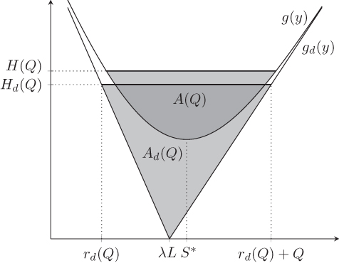
Figure 5.7
 and
and  .
.
Let ![]() be the optimal cost in the stochastic model,
be the optimal cost in the stochastic model, ![]() be the optimal controllable cost in the stochastic model, and
be the optimal controllable cost in the stochastic model, and ![]() be the optimal cost in the deterministic model. The following theorem sheds light on the relationships among these costs. The last inequality of the theorem is especially impressive, since it succinctly relates the optimal costs and solutions of the three most fundamental inventory models: the EOQ(B), the newsvendor problem, and
an
be the optimal cost in the deterministic model. The following theorem sheds light on the relationships among these costs. The last inequality of the theorem is especially impressive, since it succinctly relates the optimal costs and solutions of the three most fundamental inventory models: the EOQ(B), the newsvendor problem, and
an ![]() policy!
policy!
The sensitivity analysis result for the EOQ model (Theorem 3.2) also applies to the EOQB (see Problem 3.14); converted to the notation in this ssection, we get
The cost function turns out to be even flatter (with respect to Q) for ![]() policies:
policies:
The
question now is, how accurate is the EOQB approximation? Zheng (1992) proves a fixed worst‐case bound of ![]() on the error that results from using the EOQB
solution:
on the error that results from using the EOQB
solution:
Like many worst‐case error bounds, the bound in Theorem 5.6 overestimates the actual error bound obtained in practice. Zheng (1992) reports that, in computational results, the actual gap was less than 1% for 80.0% of the instances tested and less than 2% for 96.3%, with a maximum gap of only 2.9%. Table 5.1 reports similar results.
This raises the question of whether ![]() is the best possible bound. The answer is no: Axsäter (1996) proves that the error is no more than
is the best possible bound. The answer is no: Axsäter (1996) proves that the error is no more than ![]() , or 11.8%. This bound is tight, in the sense that there are instances whose error comes arbitrarily close to
, or 11.8%. This bound is tight, in the sense that there are instances whose error comes arbitrarily close to ![]() , but these instances use pathological demand distributions
that do not resemble real
inventory systems.
, but these instances use pathological demand distributions
that do not resemble real
inventory systems.
5.5 Exact  Problem with Discrete
Distribution
Problem with Discrete
Distribution
Suppose now that the demand is discrete:
Individual customers arrive randomly, each demanding one unit of the product. The number of demands in 1 year has a Poisson distribution
with rate ![]() . Consequently, the lead‐time demand D has a Poisson distribution with rate
. Consequently, the lead‐time demand D has a Poisson distribution with rate ![]() ; the random variable D has pmf f and cdf F.
; the random variable D has pmf f and cdf F.
Since an order is placed immediately when ![]() reaches r,
reaches r, ![]() at any time. As in the model with continuous demands in Section 5.2, the inventory position spends equal time in each of these states:
at any time. As in the model with continuous demands in Section 5.2, the inventory position spends equal time in each of these states: ![]() has a discrete uniform distribution
on the integers
has a discrete uniform distribution
on the integers ![]() , so
, so ![]() for all
for all ![]() . (See, e.g., Zipkin (2000) for a proof.) A discrete version of the conservation‐of‐flow equations
(4.41) and (4.43) hold, so when
. (See, e.g., Zipkin (2000) for a proof.) A discrete version of the conservation‐of‐flow equations
(4.41) and (4.43) hold, so when ![]() , inventory (holding and stockout) costs accumulate at a rate of
, inventory (holding and stockout) costs accumulate at a rate of ![]() , given by 5.5 using the discrete distribution for D. Therefore, the expected total cost per year is given by
, given by 5.5 using the discrete distribution for D. Therefore, the expected total cost per year is given by
which is the discrete analogue of 5.7. As before, the function ![]() is jointly convex
in Q and r.
is jointly convex
in Q and r.
Suppose
we fix Q and we want to find ![]() , the best r for that Q. To do this, we need to choose r so that
, the best r for that Q. To do this, we need to choose r so that ![]() are as small as possible. In other words, we want to find the Q best inventory positions
are as small as possible. In other words, we want to find the Q best inventory positions ![]() to minimize the sum in 5.48. Since
to minimize the sum in 5.48. Since ![]() is convex, these Q best inventory positions are nested, in the sense that, if
is convex, these Q best inventory positions are nested, in the sense that, if ![]() is optimal for Q, then either
is optimal for Q, then either ![]() or
or ![]() is optimal for
is optimal for ![]() .
.
Figure 5.8 depicts these nested inventory positions. The solid vertical lines represent the inventory positions ![]() that are optimal for Q, while the dashed lines represent possible inventory positions to add for
that are optimal for Q, while the dashed lines represent possible inventory positions to add for ![]() . The question is, which is the better inventory position to add,
. The question is, which is the better inventory position to add, ![]() (as in Figure 5.8(a)) or
(as in Figure 5.8(a)) or ![]() (Figure 5.8(b))? If
(Figure 5.8(b))? If ![]() , then we set
, then we set ![]() ;
otherwise,
;
otherwise, ![]() .
.

Figure 5.8
Determining which  y‐values are optimal given
  .
.
Note that if ![]() , then 5.48 simplifies to
, then 5.48 simplifies to
The first term is a constant, so ![]() is optimized by optimizing
is optimized by optimizing ![]() . From Theorem 4.3,
. From Theorem 4.3,
![]() , the minimizer of
, the minimizer of ![]() , is the smallest S such that
, is the smallest S such that
and the optimal r is given by
In other words, whenever the inventory position falls to ![]() or smaller, we order up to
or smaller, we order up to ![]() . This is exactly a base‐stock policy
under discrete demand. Thus, under discrete demand and continuous review, a base‐stock policy is a special case of an
. This is exactly a base‐stock policy
under discrete demand. Thus, under discrete demand and continuous review, a base‐stock policy is a special case of an ![]() policy.
policy.
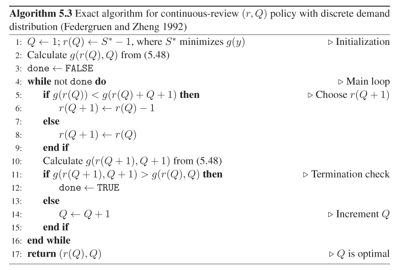
We can find the optimal Q and r recursively, as follows. We start with ![]() and set
and set ![]() , where
, where ![]() optimizes
optimizes ![]() from 5.49, i.e., where
from 5.49, i.e., where ![]() is the smallest S satisfying 5.50. We then iterate through consecutive integer values of Q, determining
is the smallest S satisfying 5.50. We then iterate through consecutive integer values of Q, determining ![]() using
using ![]() as described above. Since
as described above. Since ![]() is convex in Q, we can stop as soon as we find that
is convex in Q, we can stop as soon as we find that ![]() . This algorithm was introduced by Federgruen and Zheng (1992). Pseudocode is given in Algorithm 5.3.
. This algorithm was introduced by Federgruen and Zheng (1992). Pseudocode is given in Algorithm 5.3.
PROBLEMS
- 5.1 (Exact and Approximate r and Q: Continuous Demand) Consider an
 policy for continuous demands. Suppose the annual demand is distributed
  , the fixed cost is
  , and the holding and stockout costs are
  and
and  , respectively, per item per year. The lead time is 4 days. Find r and Q using each of the methods below.
- The EIL approximation.
- The EOQB approximation.
- The EOQ+SS approximation.
- The loss‐function approximation.
- Algorithm 5.2 for exact optimal values of r and Q.
For each method, report the values of r and Q you found, as well as the corresponding expected annual cost from 5.7.
- 5.2 (Exact and Approximate r and Q: Discrete Demand) Consider an
 policy for discrete demands. Suppose the demand has a Poisson distribution with a mean of
  units/month, the fixed cost is
  , and the holding and stockout costs are
  and
and  , respectively, per item per month. The lead‐time is 0.5 months.
- Find approximate values for r and Q by using the EOQB approximation described in Section 5.3.2, replacing
 with (4.32) when solving 5.9.
 - Find exact optimal values for r and Q using Algorithm 5.3.
For each method, report the values of r and Q you found, as well as the corresponding expected cost per week from 5.48.
- Find approximate values for r and Q by using the EOQB approximation described in Section 5.3.2, replacing
- 5.3 (
 for Automobile Components) Return to the automobile manufacturing plant from Problem 3.5. Suppose now that the rate at which the plant uses power‐lock mechanisms is stochastic and normally distributed, with a mean of 192 per day (8 per hour) and a standard deviation of 17.4 per day. Replenishment orders for power‐lock mechanisms incur a lead time of 3 days. If the plant runs out of power locks, it must expedite them from the supplier at a cost of $40 each. Using the EIL approximation for
  policies in Section 5.3.1, find approximate values for r and Q. Also report the expected total cost per week, using 5.7equation .
- The EIL approximation.
- The EOQB approximation.
- The EOQ+SS approximation.
- The loss‐function approximation.
- Algorithm 5.2 for exact optimal values of r and Q.
- 5.4 (Lackluster Video)
Lackluster Video needs to decide how may DVD copies of the new hit movie The Supply Chain's Weakest Link to stock in its stores. The company expects demand for DVD rentals for the movie over the next 90 days to be Poisson with a mean of
 per day. The length of time each renter keeps a DVD before returning it is exponential with a mean of
  days (i.e., exponential with a rate of
  ).
).Each copy purchased by the store costs c. Demands are backordered, in the sense that a customer wanting to rent the movie but finding that it is out of stock will return on another day to try again. Since this movie has been designated as a “guaranteed in stock” title, each backordered demand incurs a stockout cost of g, the cost of providing a free rental to the customer.
Assuming that backordered customers check back frequently to see whether the movie is in stock and rent it quickly when it is available, this system can be modeled as an
 queue,
where S is the number of copies of the DVD owned by the store. It can be shown that the probability of a stockout in an
queue,
where S is the number of copies of the DVD owned by the store. It can be shown that the probability of a stockout in an  queue is approximately
where
 is the standard normal cdf and
  (in queuing terminology, the “offered load”).
- Determine the optimal number of copies to purchase (S) to minimize the purchase cost and the expected stockout cost over the next 90 days using the approximation given above. (Assume that the demand after 90 days will be negligible.) Your answer should be in closed form; that is,
 .
. - Compute the optimal S assuming that
 ,
,  ,
,  , and
, and  .
. - Suppose the video store is worried about loss‐of‐goodwill costs as well as free rental costs when a demand is backordered, but it is uncomfortable estimating these costs. Instead, it would prefer to choose S so that demands are met with probability
 . Prove that the smallest such S is given by
- In two or three sentences, interpret the result from part (c) in terms of cycle and safety stock.
- Determine the optimal number of copies to purchase (S) to minimize the purchase cost and the expected stockout cost over the next 90 days using the approximation given above. (Assume that the demand after 90 days will be negligible.) Your answer should be in closed form; that is,
- 5.5 (Heating Oil Replenishments) Henry's Heating Oil company delivers oil to its customers' homes. If a customer signs up for Henry's “auto‐fill” plan, the company delivers oil to the customer's home on a regular schedule based on historical oil‐usage data for that customer. Suppose a given customer has an oil tank that holds C liters of oil. For each delivery to this customer, Henry's incurs a fixed cost of K, representing the cost of the truck, driver, and fuel required to make the delivery. Henry's will make a delivery to this customer every T days, where T is a decision variable, and at each delivery, it will deliver enough oil to fill the tank. The number of days required for the customer to use C liters of oil is a random variable, denoted X, whose pdf and cdf are f and F, respectively. If the customer uses all C liters of oil before the next delivery, Henry's must make an emergency delivery to refill the tank. For these emergency deliveries, the regular fixed cost of K does not apply, but instead Henry's incurs a penalty cost of
 . (The penalty cost is proportional to T because the more infrequent the deliveries, the more disruptive it is to Henry's delivery schedule to add an emergency delivery.) After the emergency delivery, the regular schedule resumes; that is, the next delivery will be T days after the last regular delivery. Assume the customer never needs more than one emergency shipment between two regular shipments.
- Write the expected cost per day as a function of T.
- Find an optimality condition for the delivery interval, T. You may assume that X is normally distributed and that
 .
. - Suppose
 , K = $175, p = $25, and
  . What is
  , and what is the corresponding expected cost per day?
- 5.6 (Stockout‐Constrained Service Level) Consider the EIL approximation in Section 5.3.1.
Define a new type of service level as follows:
 is the percentage of order cycles during which there are at most a stockouts, for constant
  . Suppose that we wish to enforce a service level constraint that says
  , for fixed
  . What are the optimal values of r and Q for the problem with this service level constraint?
 - 5.7 (Properties of
 ) For the exact continuous
  model in Section 5.2, prove that, for any
  :
:-

-
 ;
;  is decreasing; and
  is increasing
 -
 and
and 
-
- 5.8 (Proof of 5.32) Prove 5.32equation .
- 5.9 (Deterministic vs. Stochastic Inventory Cost Rate) Prove that
 for all
  , where
  is defined in 5.38 and
  is defined in 5.5.
 - 5.10 (Deterministic vs. Stochastic
 ) Prove that, for any
  ,
,  , where
  is defined in 5.34 and
  is its deterministic‐model analogue.
 - 5.11 (Proof of Upper Bound on
 ) Complete the proof of Theorem 5.3 by proving that
  .
. - 5.12 (Range of
 Bounds as K Changes) By Theorem 5.3,
  is contained in the interval
  , where
  satisfies
  . In this problem, you will prove that the width of this interval is bounded by a constant for all
  . (On the other hand, the constant will change as the other cost parameters change.)
- Let
 be the Q that satisfies
  . Prove that
  .
. - Prove that
 for all
  and that
  .
. - Prove that
 is an increasing function of K and converges to a constant as
  .
.Hint: Argue that it is sufficient to prove the result with respect to increases in
 rather than K.
 - Prove that
 is bounded by a constant for all
  .
.You may use the properties in Problem 5.7 without proof.
- Let
- 5.13 (EOQB Error Vanishes as
 ) Using the analysis in Section 5.4.3, prove that
  as
as  .
.
- 5.14 (EOQB as Special Case of
 ) Prove Theorem 3.5 by treating the EOQB as a special case of an
  policy, using the analysis in Section 5.4.3.
- 5.15 (
 vs.
vs.
 ) Using the analysis in Section 5.4.3, prove that
  for all
  .
. - 5.16 (Lead‐Time Demand under Stochastic Lead Times) Prove 5.24equations and 5.25.
- 5.17 (No Fixed Bound for
 ) In the exact
  model, suppose we set
  as in Section 5.2, but we set
  instead of
  . Prove that there is no fixed worst‐case bound for this approach.
- 5.18 (No Fixed Bound for EOQ+SS Approximation)
Prove that there is no fixed worst‐case error bound
for the EOQ+SS approximation for the optimal
 policy.
 - 5.19 (Joe's Corner Store with Poisson Demand) Suppose that Joe's Corner Store from Example 5.2 faces Poisson annual demand with a mean of 1300. Using Algorithm 5.3, find
 ,
,  , and
, and  .
. - 5.20 (
 with Minimum Order Quantity) Suppose that
  but there is a minimum order quantity
constraint that requires that
but there is a minimum order quantity
constraint that requires that  for some constant
  . Assume the demand has a discrete distribution. Explain how to modify Algorithm 5.3 to handle this case.
 - 5.21 (Solution in Terms of Standard Normal)
In this problem, you will investigate what happens to
 and
and  in the exact model (Section 5.2) as the lead‐time demand parameters
  and
and  change. In particular, you will investigate the relationship between the solution under
  demand and that under
  demand.
Assume that
 for some constant
  but that
  can vary independently of
  and
and  .
.Let
 be the expected cost function of the exact model under
  lead‐time demand. Let
  be the optimal parameters for this system and
  be the optimal cost; that is,
Similarly, let
 be the optimal parameters for the system with
  lead‐time demand, and let
  .
.Prove that
(5.52) (5.53)
 (5.54)
- 5.22 (Bound on
 ) Let
) Let  be the optimal order quantity for the exact model with continuous demands in Sections 5.2 and 5.4, and let
  be the optimal order quantity for the EOQB. Let
(
 does not have a precise interpretation. But it is, in a sense, a quantity for the newsvendor model that is analogous to
  for the EOQB, since in the EOQB, the optimal order quantity equals the optimal cost times
  .)
.)Prove that

Hint: First prove that

for all
 . (You may use the result of Problem 5.15 without proof.) Then use this to prove the result.
 - 5.23 (Stockout Cost without SA2)
Suppose we do not assume SA2. Show that the expected stockout cost per year under the EIL approximation has
 in the integrand instead of
  .
. - 5.24 (EIL Approximation with One‐Time Stockout Cost) Consider an inventory system that functions almost exactly like the system described in Section 5.3.1 on the EIL approximation
for the
 problem. The only difference is that, when we run out of inventory, the stockout cost p is incurred immediately, and only once, regardless of how many demands occur before the replenishment order arrives from the supplier.
- Formulate the objective function
 , analogous to 5.16.
 - Identify optimality conditions for Q and r, similar to 5.17equations and 5.18. Your optimality conditions do not need to be in closed form, i.e., they do not need to look like
 or
or  .
.
- Formulate the objective function