Chapter 4
Stochastic Inventory Models: Periodic
Review
4.1 Inventory Policies
In this chapter and the next, we will consider inventory models in which the demand is stochastic. A key concept in these chapters will be that of a policy. A policy is a simple rule that provides a solution to the inventory problem. For example, consider a periodic‐review model with fixed costs (such as the Wagner–Whitin model) but with stochastic demands. (We will examine such a model more closely in Section 4.4.) One could imagine several possible policies for this system. Here are a few:
- Every R periods, place an order for Q units.
- Whenever the inventory position falls to s, order Q units.
- Whenever the inventory position falls to s, place an order of sufficient size to bring the inventory position to S.
- Place an order whose size is equal to the first two digits of last night's lottery number. Then, wait a number of periods equal to the last two digits of the lottery number before placing another order.
Now, you probably suspect that some of these policies will perform better (in the sense of keeping costs small) than others. For example, policy 4 is probably a bad one. You probably also suspect that the performance of a policy depends on its parameters. 1 For example, policy 1 sounds reasonable, but only if we choose good values for R and Q.
It is often possible (and always desirable) to prove that a certain policy is optimal for a given problem—that no other policy (even policies that no one has thought of yet) can outperform the optimal policy, provided that we set the parameters of that policy optimally. For example, policy 3 turns out to be optimal for the model in Section 4.4: If we choose the right s and S, then we are guaranteed to incur the smallest possible expected cost.
When using policies, then, inventory optimization really has two parts: Choosing the form of the optimal policy and choosing the optimal parameters for that policy. Sometimes we can't solve one of these parts optimally, so we use approximate methods. For example, although it's possible to find the optimal s and S for the model in Section 4.4, heuristics are commonly used to find approximately optimal values. Similarly, for some problems, no one even knows the form of the optimal policy, so we simply choose a policy that seems plausible.
We'll consider periodic‐review models in this chapter. We'll first consider problems with no fixed costs (in Section 4.3) and then problems with nonzero fixed costs (in Section 4.4). In both of these sections, we'll simply choose a policy to use and focus on optimizing the policy parameters (or, in the case of finite‐horizon models, not restrict ourselves to a policy at all). This is the approach taken in the seminal paper by Arrow et al. (1951). Then, in Section 4.5, we'll prove that the policies we chose for the periodic‐review models in Sections 4.3 and 4.4 are, in fact, optimal. (We won't prove policy optimality for the continuous‐review models in Chapter 5, but those policies, too, are optimal.)
We will continue to use the same notation introduced in Chapter 3. All of the costs we discussed in Section 3.1.3 are in play, including fixed cost K,
purchase cost c,
holding cost h,
and stockout cost p.
We'll assume that K and c are nonnegative, that h and p are strictly positive, and that ![]() (otherwise it costs more to buy the product from the supplier than it does to stock out, so we should never place an order). Now, however, we'll represent the demand as a random variable D with mean
(otherwise it costs more to buy the product from the supplier than it does to stock out, so we should never place an order). Now, however, we'll represent the demand as a random variable D with mean ![]() , variance
, variance ![]() , pdf
, pdf ![]() , and cdf
, and cdf ![]() .
(D will represent demands over different time intervals in different models, but we'll make this clear in each section.) We'll usually assume that D is a continuous random variable, with a few exceptions.
.
(D will represent demands over different time intervals in different models, but we'll make this clear in each section.) We'll usually assume that D is a continuous random variable, with a few exceptions.
Throughout most of this chapter, we will assume that unmet demands are backordered. In Section 4.6, we briefly discuss the lost‐sales assumption.
Before continuing, we introduce two important concepts in stochastic inventory theory: cycle stock and safety stock. Cycle stock (or working inventory) is the inventory that is intended to meet the expected demand. Safety stock is extra inventory that's kept on hand to buffer against uncertainty. The target inventory level or order quantity set by most stochastic inventory problems can be decomposed into cycle and safety stock components. We'll see later that the cycle stock depends on the mean of the demand distribution, while the safety stock depends on the standard deviation.
4.2 Demand Processes
In real life, customers tend to arrive at a retailer at random, discrete points in time. Similarly, (some) retailers place orders to wholesalers at random, discrete times, and so on up the supply chain. One way to model these demands is using a Poisson process , which describes random arrivals to a system over time. If each customer may demand more than one unit, we might use a compound Poisson process , in which arrivals are Poisson and the number of units demanded by each customer is governed by some other probability distribution.
It
will often be convenient for us to work with continuous demand distributions
(rather than discrete distributions such as Poisson), most commonly the normal distribution with mean ![]() and variance
and variance ![]() . Sometimes, the normal distribution is used as an approximation
for the Poisson distribution, in which case
. Sometimes, the normal distribution is used as an approximation
for the Poisson distribution, in which case ![]() since the Poisson variance equals its mean. (This approximation is especially accurate when the mean is large.)
since the Poisson variance equals its mean. (This approximation is especially accurate when the mean is large.)
In the continuous‐review case, normally distributed demands mean that the demand over any t time units is normally distributed, with a mean and standard deviation that depend on t. Although it's unusual to think of demands occurring “continuously” in this way, it's a useful way to model demands over time. In the periodic‐review case, we simply assume that the demand in each time period is normally distributed.
One drawback to using the normal distribution
is that any normal random variable will sometimes have negative realizations, even though the demands that we aim to model are nonnegative. If the demand mean is much greater than its standard deviation, then the probability of negative demands is so small that we can simply ignore it. This suggests that the normal distribution is appropriate as a model for the demand only if ![]() —say, if
—say, if ![]() . If this condition fails to hold, then it is more appropriate to use a distribution whose support does not contain negative values, such as the lognormal distribution.
(If the true demands are Poisson
and we are using the normal distribution to approximate it, then another justification for the condition
. If this condition fails to hold, then it is more appropriate to use a distribution whose support does not contain negative values, such as the lognormal distribution.
(If the true demands are Poisson
and we are using the normal distribution to approximate it, then another justification for the condition ![]() is that the normal approximation for the Poisson distribution is most effective when the Poisson mean,
is that the normal approximation for the Poisson distribution is most effective when the Poisson mean, ![]() , is large, in which case
, is large, in which case ![]() , which is the standard
deviation.)
, which is the standard
deviation.)
4.3 Periodic Review with Zero Fixed Costs: Base‐Stock Policies
For the remainder of this chapter, we focus on periodic‐review models. The time horizon consists of T time periods; T can be finite or infinite. We will usually assume the lead time is zero, but in Sections 4.3.4.1 and 4.6.2, we'll discuss the implications of assuming a nonzero lead time in the case of backorders (which is easy) and lost sales (which is hard).
We'll first consider the important special case in which ![]() (in this section), and then the more general case of
(in this section), and then the more general case of ![]() (in Section 4.4). We'll also assume that the costs h, p, c, and K are constant throughout the time horizon.
(in Section 4.4). We'll also assume that the costs h, p, c, and K are constant throughout the time horizon.
We will model the time value of money by discounting future periods using a discount factor ![]() . That is, $1 spent (or received) in period
. That is, $1 spent (or received) in period ![]() is equivalent to $
is equivalent to $![]() in period t. If
in period t. If ![]() , then there is no discounting. For the single‐period and finite‐horizon
problems, our objective will be to minimize the total expected discounted cost over the horizon. However, the total cost over an infinite horizon
will be infinite if
, then there is no discounting. For the single‐period and finite‐horizon
problems, our objective will be to minimize the total expected discounted cost over the horizon. However, the total cost over an infinite horizon
will be infinite if ![]() and may still be infinite if
and may still be infinite if ![]() . Therefore, in the infinite‐horizon case, we will minimize the expected cost per period if
. Therefore, in the infinite‐horizon case, we will minimize the expected cost per period if ![]() and the total expected discounted cost over the horizon if
and the total expected discounted cost over the horizon if ![]() . (The solutions to the two problems turn out to be closely related.)
. (The solutions to the two problems turn out to be closely related.)
The sequence of events in each period t is as follows:
- The inventory level is observed.
- A replenishment order of size
 is placed and is received instantly.
 - Demand
 occurs; as much as possible is satisfied from inventory, and the rest is backordered.
 - Holding and stockout costs are assessed based on the ending inventory level.
The ending inventory level in period t (step 4) is denoted ![]() . It is equal to the starting inventory level in period
. It is equal to the starting inventory level in period ![]() (step 1) and is given by
(step 1) and is given by ![]() .
.
4.3.1 Base‐Stock Policies
Throughout Section 4.3, we'll assume that the firm follows a base‐stock policy.
2
A base‐stock policy works as follows: In each time period, we observe the current inventory position
and then place an order whose size is sufficient to bring the inventory position up to S. (We sometimes say we “order up to S.”) S is a constant—it does not depend on the current state of the system—and is known as the base‐stock level.
Base‐stock policies are optimal when ![]() ; we will prove this in Section 4.5.1. One of the earliest analyses of this type of policy is by Arrow et al. (1951).
; we will prove this in Section 4.5.1. One of the earliest analyses of this type of policy is by Arrow et al. (1951).
In multiple‐period models, the base‐stock level may be different in different periods. If the base‐stock level is the same throughout the horizon, then in every period, we simply order ![]() items. (Why?)
items. (Why?)
We will divide this problem into three cases—with ![]() ,
, ![]() , and
, and ![]() —and find the optimal base‐stock levels in each case.
—and find the optimal base‐stock levels in each case.
4.3.2 Single Period: The Newsvendor Problem
4.3.2.1 Problem Statement
Consider a firm selling a single product during a single time period. Single‐period models are most often applied to perishable products, which include (as you might expect) products such as eggs and flowers that may spoil, but also products that lose their value after a certain date, such as newspapers, high‐tech devices, and fashion goods. The key element of the model is that the firm only has one opportunity to place an order—before the random demand is observed.
Even if the firm actually sells its products over multiple periods (as is typical), the operations in subsequent periods are not linked: Excess inventory cannot be held over until the next period, nor can excess demands (that is, unmet demands are lost, not backordered). Therefore, the firm's multiperiod model can be reduced to multiple independent copies of the single‐period model presented here.
This model is one of the most fundamental stochastic inventory models, and many of the models discussed subsequently in this book use it as a starting point. It is often referred to as the newsvendor (or newsboy)
model. The story goes like this: Imagine a newsvendor who buys newspapers each day from the publisher for $0.30 each and sells them for $1.00. The daily demand for newspapers at his newsstand is normally distributed with a mean of 50 and a standard deviation of 8. If the newsvendor has unsold newspapers left at the end of the day, he cannot sell them the next day, but he can sell them back to the publisher for $0.12 (called the salvage value).
The question is: How many newspapers should he buy from the publisher each day? If he buys exactly 50, he has an equal probability of being understocked and overstocked. But it costs more to stock out than to have excess (since stocking out costs him 70 cents in lost profit while excess newspapers cost him ![]() cents each). So he should order more than 50 newspapers each day—but how many more?
cents each). So he should order more than 50 newspapers each day—but how many more?
The inventory carried by the newsvendor can be decomposed into two components: cycle stock and safety stock. As noted in Section 4.1, cycle stock is the inventory that is intended to meet the expected demand—in our example, 50—whereas safety stock is extra inventory that's kept on hand to buffer against demand uncertainty—the amount over 50 ordered by the newsvendor. We will see later that the newsvendor's cycle stock depends on the mean of the demand distribution, while the safety stock depends on the standard deviation.
It is possible for the safety stock to be negative: If stocking out is less expensive than holding extra inventory, the newsvendor would want to order fewer than 50 papers. This can actually occur in practice—for example, for expensive and highly perishable products—but it is the exception rather than the rule.
The mathematical analysis of the newsvendor problem originated with Arrow et al. (1951), though some of the ideas are much older: Edgeworth (1888) uses newsvendor‐type logic to determine the amount of cash to keep on hand at a bank to satisfy random withdrawals by patrons. Morse and Kimball (1951) introduced the name “newsboy problem,” and Porteus (2008) cites Matt Sobel as proposing the gender‐neutral term “newsvendor problem.”
As previously noted, the newsvendor model applies to perishable goods. In particular, it applies to goods that perish before the next ordering opportunity. Many perishable goods have a shelf life that exceeds the order interval: For example, a supermarket might place replenishment orders every few days for milk, which has a shelf life of a few weeks. Cases like this are much more difficult to optimize; for a more detailed discussion, see Section 16.3.2.
4.3.2.2 Formulation
As
usual, we will use h to represent the holding cost: the cost per unit of having too much inventory on hand. In the newsvendor problem, this typically consists of the purchase cost
of the unit, minus any salvage value,
but may include other costs, such as processing costs. (Since inventory cannot be carried to the next period, this cost is not technically a holding cost, though we will refer to it that way anyway.) Similarly, p represents the stockout cost: the cost per unit of having too little inventory, consisting of lost profit and loss‐of‐goodwill
costs. The holding cost is the cost per unit of positive ending inventory, while the stockout cost is the cost per unit of negative ending inventory.
The costs h and p are sometimes referred to as overage and underage costs, respectively (and some authors denote them ![]() and
and ![]() ). We can assume that the purchase cost is included in h and that its negative is included in p, and therefore, we assume that
). We can assume that the purchase cost is included in h and that its negative is included in p, and therefore, we assume that ![]() . We'll also assume the firm starts the period with
. We'll also assume the firm starts the period with ![]() , but this, too, is easy to relax (see Section 4.3.2.6). Since there is only a single period, the discount factor
, but this, too, is easy to relax (see Section 4.3.2.6). Since there is only a single period, the discount factor ![]() won't play a role in the analysis.
won't play a role in the analysis.
We will refer to the model discussed here as the implicit formulation of the newsvendor problem since the costs and revenues are not modeled explicitly but instead are accounted for in the holding and stockout costs h and p. (In contrast, see the explicit formulation in Section 4.3.2.4.)
Recall that D is a random variable that represents the demand per period. We'll assume, for now, that D has a continuous distribution. In Section 4.3.2.8, we'll modify the analysis to handle discrete demand distributions.
Our goal is to determine the base‐stock level S to minimize the expected cost in the single period. The strategy for solving this problem is first to develop an expression for the cost as a function of d (the observed demand) and S (call it ![]() ); then to determine the expected cost
); then to determine the expected cost ![]() (call it
(call it ![]() ); and then (in Section 4.3.2.3) to determine S to
minimize
); and then (in Section 4.3.2.3) to determine S to
minimize ![]() .
.
Let ![]() and
and ![]() be the on‐hand inventory and backorders, respectively, at the end of the period if the firm orders up to S and sees a demand of d units. The cost for an observed demand of d is
be the on‐hand inventory and backorders, respectively, at the end of the period if the firm orders up to S and sees a demand of d units. The cost for an observed demand of d is
Since the demand is stochastic, however, we must take an expectation over D. Let ![]() and
and ![]() be the expected on‐hand inventory and backorders if the firm orders up to S. Then,
be the expected on‐hand inventory and backorders if the firm orders up to S. Then,

Let
These functions are known as the loss function and the complementary loss function, 3 respectively. They can be defined for any probability distribution; here, we define them in terms of the demand distribution. (See Section C.3.1 for more information about these functions.) Then we can rewrite 4.3 as
This gives us three ways to write the expected cost function: using ![]() and
and ![]() 4.2, using integrals 4.3, and using loss functions 4.6. It is also common to use the following identities:
4.2, using integrals 4.3, and using loss functions 4.6. It is also common to use the following identities:
all of which follow from the fact that ![]() for all x. These let us rewrite 4.2, 4.3,
and 4.6 as
for all x. These let us rewrite 4.2, 4.3,
and 4.6 as
4.3.2.3 Optimal Solution
The derivatives of the loss function and its complement are given by
(See Problem 4.23.) Moreover, ![]() , so
, so ![]() and
and ![]() are both convex, and therefore so is
are both convex, and therefore so is ![]() .
To minimize
.
To minimize ![]() , therefore, we set its first derivative to 0. Using 4.6,
, therefore, we set its first derivative to 0. Using 4.6,
Setting this equal to 0 gives

Alternately, we can differentiate 4.12 to get
which is identical to 4.15 and so gives the same optimal solution as 4.17.
The expression for ![]() in 4.17 is an important one, so we'll state it as a theorem (which we've now proven).
in 4.17 is an important one, so we'll state it as a theorem (which we've now proven).
![]() is known as the critical ratio
(or critical fractile).
It is implicit in a result by Arrow et al. (1951) but was first formulated explicitly by Whitin (1953). Since p and h are both positive,
is known as the critical ratio
(or critical fractile).
It is implicit in a result by Arrow et al. (1951) but was first formulated explicitly by Whitin (1953). Since p and h are both positive,
so ![]() always exists.
always exists. ![]() , or the probability of no stockouts. This is known as the type‐1 service level
(see Section 4.3.4.2). Equation 4.17 then says that under the optimal solution, the type‐1 service level should be equal to the critical ratio. It is optimal to stock out in
, or the probability of no stockouts. This is known as the type‐1 service level
(see Section 4.3.4.2). Equation 4.17 then says that under the optimal solution, the type‐1 service level should be equal to the critical ratio. It is optimal to stock out in ![]() fraction of periods. To put it another way, the probability of not having a stockout is equal to the shaded area in Figure 4.1, and Theorem 4.1 says that this area should equal
fraction of periods. To put it another way, the probability of not having a stockout is equal to the shaded area in Figure 4.1, and Theorem 4.1 says that this area should equal ![]() and that the non‐shaded area should equal
and that the non‐shaded area should equal ![]() . As p increases, the critical ratio increases, so
. As p increases, the critical ratio increases, so ![]() and the type‐1 service level both increase—it is more costly to stock out, so we should do it less frequently. As h increases, the critical ratio decreases, as does
and the type‐1 service level both increase—it is more costly to stock out, so we should do it less frequently. As h increases, the critical ratio decreases, as does ![]() —it is more costly to have excess inventory, so we will order less. The type‐1 service level necessarily decreases as well.
—it is more costly to have excess inventory, so we will order less. The type‐1 service level necessarily decreases as well.

Figure 4.1 Optimal solution to newsvendor problem plotted on demand distribution.
Theorem 4.1—or one very much like it—holds for a wide range of models, not just the single‐period newsvendor model formulated here. Perhaps most importantly, a variant of the theorem still holds for the mutliperiod, infinite‐horizon version of the model; see Section 4.3.4.
4.3.2.4 Explicit Formulation
The formulation given in Sections 4.3.2.2–4.3.2.3 interprets h and p as the overage and underage costs, respectively—the cost per unit of having too much or too little inventory. The actual cost and revenue parameters are included implicitly through the overage and underage costs. For instance, in the example described in Section 4.3.2.1, there is a revenue of $1.00, a purchase cost of $0.30, and a salvage value of $0.12, but these don't appear explicitly in the expected cost function 4.2; rather, they are factored into h and p.
Instead, one can write the expected cost function explicitly using these cost parameters, and the resulting formulation is sometimes more intuitive. In particular, let r be the revenue earned per unit sold, let c be the cost per unit purchased,
and let v be the salvage value
earned for each unit of excess inventory. We assume ![]() , otherwise we earn more by salvaging a unit than by selling it, so we would never sell any items.
, otherwise we earn more by salvaging a unit than by selling it, so we would never sell any items.
Let h and p be the holding and stockout costs, but reinterpret them to exclude the costs and revenues related to selling, buying, and salvaging the inventory. For example, h might represent a storage cost or a cost to dispose of the inventory; p might represent loss of goodwill or bookkeeping costs related to unmet demands.
As before, the objective is to minimize ![]() , which should now include revenues as negative costs. We have:
, which should now include revenues as negative costs. We have:


Sometimes, this is instead formulated as a profit maximization
problem in which we maximize ![]() .
.
Since ![]() and
and ![]() are both convex, and since
are both convex, and since ![]() ,
, ![]() is convex
(and
is convex
(and ![]() is concave), so it suffices to set the first derivative of 4.19 to 0:
is concave), so it suffices to set the first derivative of 4.19 to 0:

We can translate this to the implicit version of the problem by determining the overage and underage costs (which we'll denote by ![]() and
and ![]() , respectively, since they have a slightly different meaning than h and p in the explicit formulation). For each unit of excess inventory, we incur a holding cost of h, and we paid c for the extra unit but earn v as a salvage value; therefore,
, respectively, since they have a slightly different meaning than h and p in the explicit formulation). For each unit of excess inventory, we incur a holding cost of h, and we paid c for the extra unit but earn v as a salvage value; therefore, ![]() . Similarly, for each stockout, we incur a penalty of p in addition to the lost profit
. Similarly, for each stockout, we incur a penalty of p in addition to the lost profit ![]() , so
, so ![]() . Therefore, applying 4.17, we get
. Therefore, applying 4.17, we get
which matches 4.20. The expected cost functions 4.12 and 4.19 are not equal, but they differ only by an additive constant (see Problem 4.15).
It is perfectly acceptable to set any of the cost or revenue parameters to 0 if they are negligible or should not be included in the model.
One word of caution: Avoid mixing the implicit and explicit approaches, since doing so can lead to incorrect accounting of the various costs and revenues. For example, it is a common mistake to use something like the objective function from the implicit formulation 4.3, but to add ![]() or subtract
or subtract

to reflect a purchase cost or sales revenue. If the holding and stockout costs in 4.3 are interpreted as overage and underage costs, then the purchase cost and sales revenue are already implicitly included in h and p (as they are in Example 4.1). To include them explicitly in the objective function would be to double‐count them.
For the remainder of this chapter and for most of the rest of this book, we will use the implicit formulation. An exception is Chapter 14, which uses something more like the explicit approach.
4.3.2.5 Normally Distributed Demands
In this section, we discuss results for the special case in which demands are normally distributed: ![]() , with pdf f and cdf F. We use
, with pdf f and cdf F. We use ![]() and
and ![]() to denote the pdf and cdf, respectively, of the standard normal
distribution:
to denote the pdf and cdf, respectively, of the standard normal
distribution:
We also use ![]() to denote the
to denote the ![]() th fractile of the standard normal distribution;
that is,
th fractile of the standard normal distribution;
that is, ![]() .
.
As discussed in Section 4.2, we will assume that ![]() so that the probability of negative demands is negligible.
so that the probability of negative demands is negligible.
From 4.16, we have

If we let ![]() , we have
, we have
The first term of 4.24 represents the cycle stock
—it depends only on ![]() . The second term represents the safety stock
—it depends on
. The second term represents the safety stock
—it depends on ![]() . The newsvendor problem can be thought of as a problem of setting safety stock. The firm already knows that it will need
. The newsvendor problem can be thought of as a problem of setting safety stock. The firm already knows that it will need ![]() units to satisfy the expected demand; the question is how much more to order to satisfy any demand in excess of the mean. This extra inventory is the safety stock. (See Figure 4.2.)
units to satisfy the expected demand; the question is how much more to order to satisfy any demand in excess of the mean. This extra inventory is the safety stock. (See Figure 4.2.)

Figure 4.2 Optimal solution to newsvendor problem plotted on normal demand distribution.
Note that, as discussed in Section 4.3.2.1, the safety stock is negative if ![]() since, in that case,
since, in that case, ![]() and
and ![]() .
.
We next derive an expression for the expected cost under the optimal solution, as we did with the economic order quantity (EOQ) problem in Section 3.2.3. If X is a normally distributed random variable, then its loss and complementary loss functions are given by
where ![]() and
and
(See Problem 4.22.) 4.25 and 4.26 assume ![]() ; this is true for actual demands, but it is only approximately true for the normal distribution we use to model demand.
; this is true for actual demands, but it is only approximately true for the normal distribution we use to model demand. ![]() is called the standard normal loss function;
it is equivalent to
is called the standard normal loss function;
it is equivalent to ![]() in 4.4 if X has a standard normal distribution.
in 4.4 if X has a standard normal distribution. ![]() is tabulated in many textbooks, or it can be computed explicitly as
is tabulated in many textbooks, or it can be computed explicitly as
Equation 4.28 is convenient for calculating ![]() in, say, Excel
, MATLAB
, or Python
, since these and many other environments have built‐in functions for
in, say, Excel
, MATLAB
, or Python
, since these and many other environments have built‐in functions for ![]() and
and ![]() but not
for
but not
for ![]() .
.
Then, for our problem with normally distributed demands, the cost function 4.6 becomes
for any ![]() , where
, where ![]() . From 4.24,
. From 4.24, ![]() . Then from 4.29,
. Then from 4.29,

It seems surprising at first that 4.30 depends only on ![]() , not on
, not on ![]() . But with a little reflection, this makes sense: Since the problem comes down to setting safety stock levels, only
. But with a little reflection, this makes sense: Since the problem comes down to setting safety stock levels, only ![]() should figure into the objective function. Remember that the objective function includes only holding and stockout costs—costs that result from the randomness in demand, not its magnitude.
should figure into the objective function. Remember that the objective function includes only holding and stockout costs—costs that result from the randomness in demand, not its magnitude.
Again, let's summarize the optimal order quantity and its cost in a theorem:
4.3.2.6 Nonzero Starting Inventory Level
We assumed that the firm starts the period with ![]() . In fact, this assumption is easy to relax (and it will be important to do so in the multiperiod versions of this model). If
. In fact, this assumption is easy to relax (and it will be important to do so in the multiperiod versions of this model). If ![]() , then the firm should order up to
, then the firm should order up to ![]() , as usual. But suppose
, as usual. But suppose ![]() . The firm can't order up to
. The firm can't order up to ![]() since it already has too much inventory. But should the firm order any units? By the convexity of
since it already has too much inventory. But should the firm order any units? By the convexity of ![]() , the answer is no: It would be better to leave the inventory level where it is. Therefore, the optimal order quantity at the start of the period is
, the answer is no: It would be better to leave the inventory level where it is. Therefore, the optimal order quantity at the start of the period is

4.3.2.7 Forecasting and Standard Deviations
In most real‐world settings, we do not know the demand process exactly. Instead, we generate a forecast or estimate of the demand parameters required to make inventory decisions. We'll assume the demand is normally distributed. If we knew ![]() and
and ![]() , we would simply use them in 4.24 to determine the optimal order quantity. But suppose we don't know them; instead, suppose we have observed the demand for a long time, and let
, we would simply use them in 4.24 to determine the optimal order quantity. But suppose we don't know them; instead, suppose we have observed the demand for a long time, and let ![]() be the observed demand in period t. In each period, we can generate an estimate of
be the observed demand in period t. In each period, we can generate an estimate of ![]() and
and ![]() from the historical data. There are many ways to do this (see Chapter 2); one of the simplest is to use a moving average
(Section 2.2.1) to estimate
from the historical data. There are many ways to do this (see Chapter 2); one of the simplest is to use a moving average
(Section 2.2.1) to estimate ![]() and what we might call a moving standard deviation
to estimate
and what we might call a moving standard deviation
to estimate ![]() in period t:
in period t:

To choose an order quantity in period t, we replace ![]() with
with ![]() in 4.24. However, it turns out that
in 4.24. However, it turns out that ![]() is not the right standard deviation to use in place of
is not the right standard deviation to use in place of ![]() . Instead, the correct quantity to use is
the standard deviation of the forecast error.
. Instead, the correct quantity to use is
the standard deviation of the forecast error.
Returning to our historical data, ![]() serves as a forecast for the demand in period t. The forecast error
(the forecast minus the observed demand in a given period) is a random variable, and it has a mean, denoted
serves as a forecast for the demand in period t. The forecast error
(the forecast minus the observed demand in a given period) is a random variable, and it has a mean, denoted ![]() , and a standard deviation, denoted
, and a standard deviation, denoted ![]() . The correct quantity to replace
. The correct quantity to replace ![]() with in 4.24 is
with in 4.24 is ![]() . We'll omit a rigorous explanation of why this is the case (see, e.g., Nahmias (2005, Section 2.12)), but here is the intuition. The forecasting process introduces sampling error in addition to the randomness in demand, and it is this error that the firm really needs to protect itself against using safety stock.
Suppose that the demand is very variable (
. We'll omit a rigorous explanation of why this is the case (see, e.g., Nahmias (2005, Section 2.12)), but here is the intuition. The forecasting process introduces sampling error in addition to the randomness in demand, and it is this error that the firm really needs to protect itself against using safety stock.
Suppose that the demand is very variable (![]() is large), but we are extremely good at predicting it (
is large), but we are extremely good at predicting it (![]() and
and ![]() are both small). We would need very little safety stock, because we can accurately predict how much inventory we will need. Now suppose that the demand is extremely steady (
are both small). We would need very little safety stock, because we can accurately predict how much inventory we will need. Now suppose that the demand is extremely steady (![]() is small) but that, for some reason, our forecast is always 100 units too large (
is small) but that, for some reason, our forecast is always 100 units too large (![]() is large,
is large, ![]() is small). Here, too, we need very little safety stock, because (knowing our forecast is always too large), we can simply revise our forecast downward. Finally, suppose that the demand is steady (
is small). Here, too, we need very little safety stock, because (knowing our forecast is always too large), we can simply revise our forecast downward. Finally, suppose that the demand is steady (![]() is small) but our forecasts are all over the place—sometimes high, sometimes low (
is small) but our forecasts are all over the place—sometimes high, sometimes low (![]() is small,
is small, ![]() is large). In this case, we need a lot of safety stock to protect against the uncertainty arising from our inability to predict the demand. In all of these cases, it is the standard deviation of the forecast error that drives the inventory requirement.
is large). In this case, we need a lot of safety stock to protect against the uncertainty arising from our inability to predict the demand. In all of these cases, it is the standard deviation of the forecast error that drives the inventory requirement.
Unfortunately, we don't know ![]() any more than we know
any more than we know ![]() . Instead, we can observe the forecast error
in period t,
. Instead, we can observe the forecast error
in period t,
and estimate the standard deviation of the forecast error as

where

is the estimate of the mean of the forecast error
made in period t. (If we know for sure that our forecasts are unbiased, we can replace ![]() with 0.) We then replace
with 0.) We then replace ![]() with
with ![]() in 4.24 and in the analysis that follows. Of course, if the firm uses a forecasting technique other than moving average, we can simply replace the formulas above with the appropriate ones.
in 4.24 and in the analysis that follows. Of course, if the firm uses a forecasting technique other than moving average, we can simply replace the formulas above with the appropriate ones.
Now, in nearly all of the models in this book (one exception is Section 13.2.2), we assume that the demand parameters are known and stationary. In that case, the forecast ![]() is always equal to the true demand mean
is always equal to the true demand mean ![]() , and the forecast error is
, and the forecast error is ![]() with mean 0 and standard deviation
with mean 0 and standard deviation

which converges to ![]() in the long run. Therefore,
in the long run. Therefore, ![]() and
and ![]() are the appropriate parameters to use.
are the appropriate parameters to use.
In general, one can show that ![]() for some constant c (at least for moving average
and exponential smoothing
forecasts; see, e.g., Hax and Candea (1984, p. 174), or Nahmias (2005, Appendix 2‐A)), so in some sense the distinction between the standard deviation of the demand and that of the forecast error is academic, but it's still worth drawing.
for some constant c (at least for moving average
and exponential smoothing
forecasts; see, e.g., Hax and Candea (1984, p. 174), or Nahmias (2005, Appendix 2‐A)), so in some sense the distinction between the standard deviation of the demand and that of the forecast error is academic, but it's still worth drawing.
This analysis assumes that ![]() , i.e., the forecast is unbiased. If it is not, we should also use
, i.e., the forecast is unbiased. If it is not, we should also use ![]() in place of
in place of ![]() in 4.24: If our forecasts tend to be too high (
in 4.24: If our forecasts tend to be too high (![]() ), then we should reduce the estimate of the mean demand to account for this; and if our forecasts are low (
), then we should reduce the estimate of the mean demand to account for this; and if our forecasts are low (![]() ), we should
increase it.
), we should
increase it.
4.3.2.8 Discrete Demand Distributions
Suppose now that D is discrete. In this case, 4.3 becomes

The expected cost can still be expressed in terms of loss functions, keeping 4.6 as is but replacing the definitions of ![]() and
and ![]() in 4.4 and 4.5
with
in 4.4 and 4.5
with


(See Section C.3.4 for more on loss functions for discrete distributions.)

Figure 4.3
 and
and  .
.
The expected cost function ![]() is still convex
but no longer differentiable; it is piecewise‐linear,
with breakpoints at each positive integer. (Why?) Therefore, we cannot use derivatives to minimize it. Instead, we can use finite differences
. A finite difference is very similar to a derivative except that, instead of measuring the change in the function as the variable changes infinitesimally, it measures the change as the variable changes by one unit. Let
is still convex
but no longer differentiable; it is piecewise‐linear,
with breakpoints at each positive integer. (Why?) Therefore, we cannot use derivatives to minimize it. Instead, we can use finite differences
. A finite difference is very similar to a derivative except that, instead of measuring the change in the function as the variable changes infinitesimally, it measures the change as the variable changes by one unit. Let
Imagine starting at ![]() and increasing S one unit at a time. If
and increasing S one unit at a time. If ![]() , i.e.,
, i.e., ![]() , then we would want to increase S to
, then we would want to increase S to ![]() to bring the cost down. Since
to bring the cost down. Since ![]() is convex,
is convex, ![]() is the smallest S such that
is the smallest S such that ![]() . (See Figure 4.3.) Well,
. (See Figure 4.3.) Well,

Therefore, ![]() is the smallest S such that
is the smallest S such that ![]() ; that is:
; that is:
Unless we get lucky, there is no S such that ![]() equals the critical ratio,
as it does for continuous demands, so instead we “round up” to the next greater integer. That is, if
equals the critical ratio,
as it does for continuous demands, so instead we “round up” to the next greater integer. That is, if ![]() , there is no need to evaluate both
, there is no need to evaluate both ![]() and
and ![]() ;
; ![]() will always be smaller. Note, however, that this does not hold when the demands are continuous but the order quantities must be discrete;
see Problem 4.16.
will always be smaller. Note, however, that this does not hold when the demands are continuous but the order quantities must be discrete;
see Problem 4.16.
4.3.3 Finite Horizon
Now
consider a multiple‐period problem consisting of a finite number of periods, T. Suppose we are at the beginning of period t. Do we need to know the history of the system (e.g., order quantities and demands through period ![]() ) in order to make an optimal inventory decision in period t? The answer is no: All of the information we need to make the inventory decision is contained in a single quantity—the starting inventory level, which equals the ending inventory level in the previous period,
) in order to make an optimal inventory decision in period t? The answer is no: All of the information we need to make the inventory decision is contained in a single quantity—the starting inventory level, which equals the ending inventory level in the previous period, ![]() . Moreover, once we decide how much to order, we can easily calculate the probability distribution of the ending inventory level in period t (as we'll see below). This suggests that the periods can be optimized recursively—in particular, using dynamic programming (DP). Just as in the DP algorithm we used for the Wagner–Whitin problem (Section 3.7.3), this DP will make inventory decisions for period t, assuming that optimal decisions have already been made for periods
. Moreover, once we decide how much to order, we can easily calculate the probability distribution of the ending inventory level in period t (as we'll see below). This suggests that the periods can be optimized recursively—in particular, using dynamic programming (DP). Just as in the DP algorithm we used for the Wagner–Whitin problem (Section 3.7.3), this DP will make inventory decisions for period t, assuming that optimal decisions have already been made for periods ![]() and using the cost of those optimal decisions to calculate the cost of the decisions in period t. However, in this DP, the optimal decisions in period t will depend on a random state variable (in particular,
and using the cost of those optimal decisions to calculate the cost of the decisions in period t. However, in this DP, the optimal decisions in period t will depend on a random state variable (in particular, ![]() ), whereas the decisions in the Wagner–Whitin DP depended only on the period, t.
), whereas the decisions in the Wagner–Whitin DP depended only on the period, t.
First consider what happens at the end of the time horizon. Presumably, on‐hand units
and backorders
must be treated differently now that the horizon has ended than they would be during the horizon. The terminal cost function,
denoted ![]() , represents the additional cost incurred at the end of the horizon if we end the horizon with inventory level x. For example, we may incur a terminal holding cost
, represents the additional cost incurred at the end of the horizon if we end the horizon with inventory level x. For example, we may incur a terminal holding cost
![]() for on‐hand units that must be disposed of, and a terminal stockout cost
for on‐hand units that must be disposed of, and a terminal stockout cost
![]() for backorders that must be satisfied through overtime or other expensive measures. Then
for backorders that must be satisfied through overtime or other expensive measures. Then ![]() . Or, maybe we can salvage excess units at the end of the horizon for a revenue of
. Or, maybe we can salvage excess units at the end of the horizon for a revenue of ![]() per unit, in which
case
per unit, in which
case ![]() .
.
Let ![]() be the optimal expected cost in periods
be the optimal expected cost in periods ![]() if we begin period t with an inventory level of x (and act optimally thereafter). We can define
if we begin period t with an inventory level of x (and act optimally thereafter). We can define ![]() recursively in terms of
recursively in terms of ![]() for later periods s. In each period t, we need to decide how much to order, but we will express this optimization problem not in terms of the order quantity Q, but the order‐up‐to level
y, defined as
for later periods s. In each period t, we need to decide how much to order, but we will express this optimization problem not in terms of the order quantity Q, but the order‐up‐to level
y, defined as ![]() .
4
In particular:
.
4
In particular:
where
is the single‐period expected cost function (see 4.3 and 4.6). The minimization considers all possible order‐up‐to levels ![]() (since Q must be nonnegative) and, for each, calculates the sum of the cost to order
(since Q must be nonnegative) and, for each, calculates the sum of the cost to order ![]() units, the expected cost in period t, and the expected discounted future cost. Note that if we order up to y in period t, then the starting inventory level in period
units, the expected cost in period t, and the expected discounted future cost. Note that if we order up to y in period t, then the starting inventory level in period ![]() will be
will be ![]() , where D is the (random) demand in period t; therefore, the (random) cost in periods
, where D is the (random) demand in period t; therefore, the (random) cost in periods ![]() equals
equals ![]() .
.
The DP algorithm for the finite‐horizon problem is given in Algorithm 4.1. The optimal expected cost for the entire horizon is given by ![]() , where
, where ![]() is the inventory level that the system starts with at the beginning of period 1.
is the inventory level that the system starts with at the beginning of period 1.

One way to think about this DP is as follows. Imagine a spreadsheet whose columns correspond to the periods ![]() and whose rows correspond to the possible values of x. The value in cell
and whose rows correspond to the possible values of x. The value in cell ![]() equals
equals ![]() . We start by filling in the
. We start by filling in the ![]() values in the last column, one for each value of x. Then, we calculate the cells in column T: For each x, we calculate
values in the last column, one for each value of x. Then, we calculate the cells in column T: For each x, we calculate ![]() using 4.36—which requires us to look in column
using 4.36—which requires us to look in column ![]() for the
for the ![]() values—and write the result in cell
values—and write the result in cell ![]() . Then we calculate the cells in column
. Then we calculate the cells in column ![]() , using the values in column T, and so on, until we solve period 1. Also imagine a second spreadsheet with identical structure but whose cells contain
, using the values in column T, and so on, until we solve period 1. Also imagine a second spreadsheet with identical structure but whose cells contain ![]() rather than
rather than ![]() .
.

The completed spreadsheets tell the firm everything it needs to know about optimally managing the inventory system. If it finds itself with an inventory level of x at the start of period t, it simply looks in the second spreadsheet and orders up to the ![]() value that is found in cell
value that is found in cell ![]() . (The corresponding cell in the first spreadsheet tells the expected current and future cost of this action.)
. (The corresponding cell in the first spreadsheet tells the expected current and future cost of this action.)
Two problems with this approach bear mentioning. First, the DP calculates ![]() “for all x.” But x can potentially become arbitrarily large or small, depending on the values we choose for y and on the random demands. For example, if
“for all x.” But x can potentially become arbitrarily large or small, depending on the values we choose for y and on the random demands. For example, if ![]() and
and ![]() , it is possible (although extremely unlikely) that
, it is possible (although extremely unlikely) that ![]() will equal
will equal ![]() , so our spreadsheet should extend at least this far. Of course, this is neither practical nor essential (since the probability is so low), so we typically truncate
the state space to consider only “reasonable” x values. (The definition of “reasonable” depends on the specific problem at hand.)
, so our spreadsheet should extend at least this far. Of course, this is neither practical nor essential (since the probability is so low), so we typically truncate
the state space to consider only “reasonable” x values. (The definition of “reasonable” depends on the specific problem at hand.)
Second, even if we consider only a reasonably narrow range of x values, if D has a continuous distribution, there are still an infinite number of possible inventory levels to consider. This problem is typically addressed by discretizing
the demand distribution so we consider only a finite number of possible demand values. The granularity of the discretization (e.g., do we round demands to the nearest integer? to the nearest 0.001? the nearest ![]() ?) again depends on the specific problem. In general, larger ranges of x values and smaller granularity result in more accurate solutions but longer run times.
?) again depends on the specific problem. In general, larger ranges of x values and smaller granularity result in more accurate solutions but longer run times.
Even after we resolve these two problems, this approach is still somewhat unsatisfying, at least from a managerial point of view. The spreadsheets described above will work, but they are fairly cumbersome. It would be nice if we could boil the information contained in the spreadsheets down into a simple policy. To that end, let's look more closely at the results of the DP.
Figure 4.4 plots ![]() for three different periods t and for a range of x values for a particular instance of the problem.
5
Essentially, each curve contains the data from a column in the second spreadsheet. Notice that all three curves are flat for a while and then climb linearly along the line
for three different periods t and for a range of x values for a particular instance of the problem.
5
Essentially, each curve contains the data from a column in the second spreadsheet. Notice that all three curves are flat for a while and then climb linearly along the line ![]() . That is, for each t, there exists some value
. That is, for each t, there exists some value ![]() such that, for
such that, for ![]() , we have
, we have ![]() , and for
, and for ![]() , we have
, we have ![]() . (In particular,
. (In particular, ![]() ,
, ![]() ,
, ![]() .) In other words, these curves each depict a base‐stock policy!
In fact, we will prove in Section 4.5.1.2 that a base‐stock policy is optimal in every period of the finite‐horizon model presented here—the pattern suggested by Figure 4.4 always holds.
.) In other words, these curves each depict a base‐stock policy!
In fact, we will prove in Section 4.5.1.2 that a base‐stock policy is optimal in every period of the finite‐horizon model presented here—the pattern suggested by Figure 4.4 always holds.

Figure 4.4
DP results,  :
:  .
.
Recognizing the optimality of a base‐stock policy has simplified the results: We don't need the entire ![]() spreadsheet to tell us how to act in each period, we just need a list of
spreadsheet to tell us how to act in each period, we just need a list of ![]() values—the optimal base‐stock level
for each period t. In general, these can be different for different periods, as suggested by Figure 4.4, although in some special cases, the same base‐stock level is optimal in every period (see Section 4.5.1.2). However, base‐stock optimality has not simplified the computation required to determine the optimal policy—we still need to solve the DP to find the optimal base‐stock levels in each period. In particular,
values—the optimal base‐stock level
for each period t. In general, these can be different for different periods, as suggested by Figure 4.4, although in some special cases, the same base‐stock level is optimal in every period (see Section 4.5.1.2). However, base‐stock optimality has not simplified the computation required to determine the optimal policy—we still need to solve the DP to find the optimal base‐stock levels in each period. In particular, ![]() is equal to
is equal to ![]() , or, assuming we have truncated the range of possible x values,
, or, assuming we have truncated the range of possible x values, ![]() equals
equals ![]() for the smallest x value
considered.
for the smallest x value
considered.
4.3.4 Infinite Horizon
Our third and final variety of periodic‐review models with no fixed costs is the case in which ![]() . This problem is sometimes referred to as the infinite‐horizon newsvendor model.
If the number of periods is infinite, then the total expected cost across the horizon may be infinite, too. (It certainly will be if
. This problem is sometimes referred to as the infinite‐horizon newsvendor model.
If the number of periods is infinite, then the total expected cost across the horizon may be infinite, too. (It certainly will be if ![]() .) An alternate objective is to minimize the expected cost per period. The former case is known as the discounted‐cost criterion,
while the latter is known as the average‐cost criterion.
We'll consider the average‐cost criterion first, then the discounted‐cost criterion.
.) An alternate objective is to minimize the expected cost per period. The former case is known as the discounted‐cost criterion,
while the latter is known as the average‐cost criterion.
We'll consider the average‐cost criterion first, then the discounted‐cost criterion.
Under
the average‐cost criterion, we assume ![]() . The expected cost in a given period if we use base‐stock level S is given by
. The expected cost in a given period if we use base‐stock level S is given by
This is exactly the same expected cost function as in the single‐period model of Section 4.3.2. Therefore, the same base‐stock level—given in Theorem 4.1—is optimal, in every period!
In formulating 4.38, we glossed over two potentially problematic issues. First, why didn't we account for the purchase cost
c, and second, why didn't we account for the cost in future periods? Well, in the long run, the expected number of units ordered is the same—![]() —no matter what S we choose. And since
—no matter what S we choose. And since ![]() , the timing of our orders does not affect the purchase cost. Therefore, the expected purchase cost per period is independent of S.
, the timing of our orders does not affect the purchase cost. Therefore, the expected purchase cost per period is independent of S.
What about future periods? In 4.38, we didn't account for the impact of our choice of S on future periods. Is this approach sound, or do we need to account for the future cost, as in the finite‐horizon DP model of Section 4.3.3? For example, if we start period t with ![]() , then the expected cost in period t is
, then the expected cost in period t is ![]() rather than
rather than ![]() . In this case, 4.38 would give an incomplete picture of the expected cost in period t since it assumes we can always order up to S. This suggests that we cannot optimize the periods independently. However, as long as
. In this case, 4.38 would give an incomplete picture of the expected cost in period t since it assumes we can always order up to S. This suggests that we cannot optimize the periods independently. However, as long as ![]() , we can be sure that the system starts period
, we can be sure that the system starts period ![]() with
with ![]() . (Why?) Therefore, no matter what value we choose for
. (Why?) Therefore, no matter what value we choose for ![]() , we know that we can always order up to
, we know that we can always order up to ![]() in period
in period ![]() . And, as we will see in Section 4.5.1.3, the same base‐stock level is optimal in every period. Therefore,
. And, as we will see in Section 4.5.1.3, the same base‐stock level is optimal in every period. Therefore, ![]() , so
, so ![]() and we can optimize 4.38 to find the optimal base‐stock
level.
and we can optimize 4.38 to find the optimal base‐stock
level.
Now
suppose ![]() , i.e., consider the discounted‐cost criterion. Since the timing of orders now affects the cost, 4.38 is no longer valid. However, the solution turns out to be nearly as simple: The optimal base‐stock level is the same in every period, and it is given by
, i.e., consider the discounted‐cost criterion. Since the timing of orders now affects the cost, 4.38 is no longer valid. However, the solution turns out to be nearly as simple: The optimal base‐stock level is the same in every period, and it is given by
(We omit the proof.)
We summarize these conclusions in the following theorem:
Note that this theorem holds for both ![]() and
and ![]() , i.e., for both the average‐ and discounted‐cost criteria.
, i.e., for both the average‐ and discounted‐cost criteria.
If demand is normally distributed,
then the results from Section 4.3.2.5 still hold, after modifying to account for ![]() . In particular,
. In particular,
where ![]() . The comments on forecasting in Section 4.3.2.7 also apply here.
. The comments on forecasting in Section 4.3.2.7 also apply here.
4.3.4.1 Lead Times and Reorder Intervals
So far, we have assumed that the lead time is 0 and that the reorder interval
—the number of periods that elapse between orders—is 1. (The reorder interval is sometimes called the review period.)
In this section, we relax those assumptions to allow the lead time to be nonzero and the reorder interval to be greater than 1. In general, we define the lead‐time demand
as the cumulative demand in ![]() consecutive periods. In the newsvendor problem
in Section 4.3.2,
consecutive periods. In the newsvendor problem
in Section 4.3.2, ![]() and
and ![]() , so the lead‐time demand is just the demand in a single period.
, so the lead‐time demand is just the demand in a single period.
The sequence of events is the same as that on page 5. In the discussion that follows, we will use the following notation:
|
|
= ending inventory level (after step 4 of sequence of events) in period t |
|
|
= inventory position after order is placed but before demand is observed |
| (after step 2 of sequence of events) in period t | |
|
|
= demand in period t |
|
|
= cumulative demand in periods |
|
|
|
|
|
= cumulative demand in |
|
|
= pdf/pmf and cdf of |
|
|
= loss function and complementary loss function of |
For
the moment, assume that the reorder interval R equals 1, but allow an L‐period lead time, ![]() . That is, an order placed in period t (in step 2 of the sequence of events) is received in step 2 of period
. That is, an order placed in period t (in step 2 of the sequence of events) is received in step 2 of period ![]() . From step 4 of the sequence of events, the holding and stockout costs are incurred based on the ending inventory level,
. From step 4 of the sequence of events, the holding and stockout costs are incurred based on the ending inventory level, ![]() , a random variable; therefore, to calculate the expected holding and stockout costs, we need to know the distribution of
, a random variable; therefore, to calculate the expected holding and stockout costs, we need to know the distribution of ![]() , which in turn depends on the inventory policy parameters (e.g., S). The distribution of
, which in turn depends on the inventory policy parameters (e.g., S). The distribution of ![]() is not obvious, because
is not obvious, because ![]() depends on both the random demand
and the inventory actions governed by S. Worse still, there is a delayed reaction: Inventory decisions made in period t do not have an effect on
depends on both the random demand
and the inventory actions governed by S. Worse still, there is a delayed reaction: Inventory decisions made in period t do not have an effect on ![]() until period
until period ![]() . In the intervening periods, other orders may have arrived (increasing the inventory level) and demands will have occurred (decreasing the inventory level).
. In the intervening periods, other orders may have arrived (increasing the inventory level) and demands will have occurred (decreasing the inventory level).
The solution to this problem is to relate the inventory level at time ![]() to the inventory position at time t (which we know, in the case of a base‐stock policy) and to the demand during periods
to the inventory position at time t (which we know, in the case of a base‐stock policy) and to the demand during periods ![]() (whose probability distribution we know). In particular, the ending inventory level in period
(whose probability distribution we know). In particular, the ending inventory level in period ![]() is given by
is given by
Why is 4.41 true? Well, all of the items included in ![]() —including items on hand and on order—will have arrived by period
—including items on hand and on order—will have arrived by period ![]() . Moreover, no items ordered after period t will have arrived by period
. Moreover, no items ordered after period t will have arrived by period ![]() . Therefore, all items that are on hand or on order in period t will be included in the ending inventory level in period
. Therefore, all items that are on hand or on order in period t will be included in the ending inventory level in period ![]() , except for the
, except for the ![]() items that have since been demanded. (See Figure 4.5.) Another way to think of this is that if the inventory position in period t is
items that have since been demanded. (See Figure 4.5.) Another way to think of this is that if the inventory position in period t is ![]() and there is no demand during
and there is no demand during ![]() , then the inventory level in period
, then the inventory level in period ![]() will be
will be ![]() ; and if some demand does occur, then
; and if some demand does occur, then ![]() will be
will be ![]() minus that demand.
minus that demand.

Figure 4.5
Inventory dynamics. All items on order or on hand in period t have arrived by period  . Items ordered before
  arrive before t, and items ordered after t arrive after
  . In the figure,
  .
.
Equation 4.41 is a very important equation. It applies to the periodic‐review models in this chapter and—in modified form—to the continuous‐review models in Chapter 5. The idea dates back to Scarf (1960); Zipkin (2000) refers to it as a conservation of flow equation.
Note that 4.41 only holds for the lead time L; that is, in general,
This is because some of the units included in ![]() may not be delivered by period
may not be delivered by period ![]() (if
(if ![]() ), or some units ordered after period t may have been delivered by period
), or some units ordered after period t may have been delivered by period ![]() (if
(if ![]() ).
).
In steady state, we can drop the time indices from 4.41 and write
where ![]() is a random variable representing the lead‐time demand.
(We're omitting some of the probabilistic arguments necessary to justify the move from 4.41 to 4.43. See, for example, Galliher et al. (1959) and Zipkin (1986b).) If
is a random variable representing the lead‐time demand.
(We're omitting some of the probabilistic arguments necessary to justify the move from 4.41 to 4.43. See, for example, Galliher et al. (1959) and Zipkin (1986b).) If ![]() , then 4.41 simply says that the ending inventory in period t equals the inventory position after the order minus the demand in the
period.
, then 4.41 simply says that the ending inventory in period t equals the inventory position after the order minus the demand in the
period.
Let us apply this insight to the infinite‐horizon base‐stock problem under the average‐cost criterion
in Section 4.3.4. (Continue to assume that ![]() .) Since this is a base‐stock policy,
.) Since this is a base‐stock policy, ![]() in every period t. Therefore,
in every period t. Therefore,
or in steady state,
In other words, the pdf of ![]() is
is
The expected cost is still given by 4.38, and Theorem 4.4 still gives the optimal base‐stock level, with ![]() ,
, ![]() ,
, ![]() , and
, and ![]() replaced by
replaced by ![]() ,
, ![]() ,
, ![]() , and
, and ![]() . In essence, we have shifted the accounting so that actions taken in period t do not incur costs until period
. In essence, we have shifted the accounting so that actions taken in period t do not incur costs until period ![]() , though all of that logic is buried in the expectations in 4.38.
, though all of that logic is buried in the expectations in 4.38.
For normally distributed demands, Theorem 4.4 says that
where ![]() and
and ![]() refer to the demand per period (and so
refer to the demand per period (and so ![]() is the mean and
is the mean and ![]() is the standard deviation of lead‐time demand).
In 4.46,
is the standard deviation of lead‐time demand).
In 4.46, ![]() is the cycle stock
and
is the cycle stock
and ![]() is the safety stock.
The safety stock is held to protect against fluctuations in lead time demand,
which is why the safety stock component uses the standard deviation of lead time demand. The reason the cycle stock level depends on the lead time, too,
is that the base‐stock level refers to the inventory position
—so if the lead time is 4 weeks, we always want 4 weeks' worth of cycle stock in the pipeline plus 1 week's worth on
hand.
is the safety stock.
The safety stock is held to protect against fluctuations in lead time demand,
which is why the safety stock component uses the standard deviation of lead time demand. The reason the cycle stock level depends on the lead time, too,
is that the base‐stock level refers to the inventory position
—so if the lead time is 4 weeks, we always want 4 weeks' worth of cycle stock in the pipeline plus 1 week's worth on
hand.
Now let's generalize this logic to allow a reorder interval of ![]() , so that orders are placed every R periods. Continue to assume that the lead time is
, so that orders are placed every R periods. Continue to assume that the lead time is ![]() . The conservation‐of‐flow argument now goes as follows: Assume that period t is an order period and that
. The conservation‐of‐flow argument now goes as follows: Assume that period t is an order period and that ![]() . All items included in
. All items included in ![]() will have arrived by period
will have arrived by period ![]() , and therefore by period
, and therefore by period ![]() . No items ordered after period t will have arrived by period
. No items ordered after period t will have arrived by period ![]() (because any such items would have been ordered in period
(because any such items would have been ordered in period ![]() at the earliest), or therefore by period
at the earliest), or therefore by period ![]() . Therefore, the ending inventory level in period
. Therefore, the ending inventory level in period ![]() equals
equals ![]() minus the demand in periods
minus the demand in periods ![]() :
:
For a base‐stock policy, ![]() , so we have
, so we have
if t is an order period. Therefore, the expected cost is

where ![]() is the newsvendor cost function 4.3 with
is the newsvendor cost function 4.3 with ![]() replaced by
replaced by ![]() . In general, this cost function must be optimized numerically to find the optimal base‐stock level,
. In general, this cost function must be optimized numerically to find the optimal base‐stock level, ![]() .
.
Note that if ![]() , then 4.47 and 4.48 reduce to 4.41 and 4.44, respectively, and 4.49 reduces
to 4.3.
, then 4.47 and 4.48 reduce to 4.41 and 4.44, respectively, and 4.49 reduces
to 4.3.
4.3.4.2 Service Levels
The service level measures how successful an inventory policy is at satisfying the demand. There are many definitions of service level. The two most common are as follows:
- Type‐1 service level : the percentage of order cycles during which no stockout occurs, sometimes called the cycle service level , denoted A.
- Type‐2 service level : the percentage of demand that is met from stock, sometimes called the fill rate , denoted B.
(An order cycle
is the interval between two consecutive orders, or order arrivals. For base‐stock policies, the duration of each order cycle is equal to the reorder interval,
R. For ![]() policies, and for the continuous‐review models
in Chapter 5, the length of an order cycle is
stochastic.)
policies, and for the continuous‐review models
in Chapter 5, the length of an order cycle is
stochastic.)
For example, suppose there are 3 periods with the demands and stockouts given in Table 4.1. Then the type‐1 service level A is 67% (because we stocked out in 1 of 3 periods), while the type‐2 service level B is 90% (because we filled 450 out of 500 demands). In theory, the type‐1 service level can be greater than the type‐2 service level, but this rarely happens since the type‐1 service level is a more stringent measure—any cycle during which a stockout occurs is counted as a “failure,” rather than just counting the individual stockouts as failures. (The type‐1 service level would be greater than the type‐2 service level if, for example, stockouts occur very rarely, but when they do, the number of stockouts is very large.)
Table 4.1 Sample demands and stockouts.
| Period | Demand | Stockouts |
| 1 | 150 | 0 |
| 2 | 100 | 0 |
| 3 | 250 | 50 |
Focusing
now on base‐stock policies, assume that the lead time is ![]() periods. If the review period is
periods. If the review period is ![]() (see Section 4.3.4.1), the type‐1 service level is easy to calculate: By 4.45, no stockout will occur in a given period if and only if the lead‐time demand
for the interval ending at that period is less than or equal to S, i.e.,
(see Section 4.3.4.1), the type‐1 service level is easy to calculate: By 4.45, no stockout will occur in a given period if and only if the lead‐time demand
for the interval ending at that period is less than or equal to S, i.e., ![]() . If
. If ![]() , the type‐1 service level is the probability that there are no stockouts in an order cycle, i.e., over the R periods between two order arrivals. No stockout occurs in a cycle if and only if the inventory level at the end of the cycle (just before the next order arrival) is positive. By 4.48, this inventory level is positive if and only if
, the type‐1 service level is the probability that there are no stockouts in an order cycle, i.e., over the R periods between two order arrivals. No stockout occurs in a cycle if and only if the inventory level at the end of the cycle (just before the next order arrival) is positive. By 4.48, this inventory level is positive if and only if ![]() , which occurs with probability
, which occurs with probability ![]() . To summarize:
. To summarize:
The type‐2 service level is a bit trickier. The type‐2 service level is
We will start by making two simplifying assumptions to derive an approximate expression for the type‐2 service level, then relax one and then finally both assumptions to obtain another approximation and an exact expression.
- Simplifying Assumption 1 (SA1): Backorders never last for more than one order cycle. That is, each arriving order is large enough to clear all existing backorders.
-
Simplifying Assumption 2 (SA2):

SA1 is reasonable when S is sufficiently high, as it usually is in practice. SA2 is not true, of course, since ![]() in general for random variables X and Y; we will explore the loss of accuracy caused by this assumption later in this section. We will use
in general for random variables X and Y; we will explore the loss of accuracy caused by this assumption later in this section. We will use ![]() to denote the type‐2 service level under SA1 and SA2,
to denote the type‐2 service level under SA1 and SA2, ![]() to denote that under SA2 only, and B to denote the exact type‐2 service level that assumes neither.
to denote that under SA2 only, and B to denote the exact type‐2 service level that assumes neither.
Under SA1 and SA2, we have

where the second equality follows from the fact that each cycle lasts exactly R periods. Assume that an order is placed in period t and consider the cycle that begins in period ![]() and ends in period
and ends in period ![]() . After the order arrives in period
. After the order arrives in period ![]() , the inventory level is positive (by SA1), so the number of stockouts in the cycle equals
, the inventory level is positive (by SA1), so the number of stockouts in the cycle equals ![]() , using the notation in Section 4.3.4.1. Therefore,
, using the notation in Section 4.3.4.1. Therefore,

where the second equality follows from 4.48. Therefore,
Johnson et al. (1995) and subsequent authors refer to this as the “traditional approach.”
Now relax SA1. We can no longer calculate the expected number of stockouts in a cycle using the inventory level at the end of the cycle because not all of the “negative” items in ![]() are stockouts from the current cycle; some may be left over from the previous cycle. Therefore, we must account for these items more carefully.
are stockouts from the current cycle; some may be left over from the previous cycle. Therefore, we must account for these items more carefully.
Suppose period t is an order period. Let's focus on the cycle that begins in period ![]() and ends in period
and ends in period ![]() . After the order arrives in
. After the order arrives in ![]() , no additional orders arrive in this cycle. Therefore, the number of demands met from stock during this cycle equals the difference between the on‐hand inventory immediately after the order arrival in period
, no additional orders arrive in this cycle. Therefore, the number of demands met from stock during this cycle equals the difference between the on‐hand inventory immediately after the order arrival in period ![]() (call this
(call this ![]() ) and the on‐hand inventory at the end of period
) and the on‐hand inventory at the end of period ![]() (call this
(call this ![]() ). Moreover, the expected demand during the cycle is
). Moreover, the expected demand during the cycle is ![]() . Therefore,
. Therefore,

It remains to evaluate ![]() and
and ![]() . First,
. First, ![]() , where X is the inventory level immediately after the order arrival in period
, where X is the inventory level immediately after the order arrival in period ![]() . Then
. Then
since ![]() by 4.48. Therefore,
by 4.48. Therefore,
If ![]() , then the right‐hand side of 4.53 is S (since
, then the right‐hand side of 4.53 is S (since ![]() ), and in 4.54,
), and in 4.54, ![]() since (
since (![]() ).
).
Similarly,
Therefore,
where ![]() if
if ![]() .
.
This approach is due to Hadley and Whitin (1963); see also Johnson et al. (1995), Zhang and Zhang (2007), and Teunter (2009). For another, equivalent, formula for the type‐2 service level under SA2, see Problem 4.17.
Since S is chosen to cover ![]() periods of demand, we would expect the number of stockouts over L periods to be negligible; put another way,
periods of demand, we would expect the number of stockouts over L periods to be negligible; put another way,
Therefore, from 4.55,

which provides another justification of 4.52.
Finally, let us relax both SA1 and SA2 to derive the exact fill rate. As above, assume that t is an order period, and let X be the inventory level after the order arrives at the start of period ![]() . First assume that
. First assume that ![]() . Then from 4.53,
. Then from 4.53, ![]() , i.e., the pdf of X is
, i.e., the pdf of X is ![]() . We will evaluate 4.50 by conditioning on X: By the law of total expectation
,
. We will evaluate 4.50 by conditioning on X: By the law of total expectation
,

In the last equality, the change in the lower limit of the first integral comes from the fact that ![]() for
for ![]() . If
. If ![]() , then
, then ![]() , and 4.56 becomes
, and 4.56 becomes
If the demands are discrete, the integrals in 4.56 and 4.57 are replaced by sums; see Babiloni et al. (2012).
We summarize the expressions for the type‐2 service level in the following theorem.
Theorem 4.6 holds for both continuous and discrete demands, with the integrals in 4.61 replaced by sums.
Service levels are an important performance measure once the system has been optimized, but they also often play a key role in the optimization itself. The main reason for this is that the stockout penalty p is difficult to estimate, and so it is often preferable to ignore stockouts in the objective function and instead limit them in a constraint, via the service level. That is, we solve a problem of the form
The objective function comes from 4.2, ignoring the stockout cost. Since ![]() and the service levels are all increasing functions of S, this optimization problem amounts to finding S such that the constraint holds as an equality.
and the service levels are all increasing functions of S, this optimization problem amounts to finding S such that the constraint holds as an equality.
To optimize the base‐stock level subject to the type‐1 service‐level constraint 4.63, we simply have
Since the expressions for the type‐2 service level above are more complex than those for type‐1, optimizing subject to 4.64 usually requires an iterative search to find the S that satisfies ![]() in one of the (approximate or exact) expressions for B
Theorem 4.6.
in one of the (approximate or exact) expressions for B
Theorem 4.6.
4.4 Periodic Review with Nonzero Fixed Costs:  Policies
4.4.1  Policies
We now consider the more general case in which the fixed cost
K may be nonzero. If ![]() , it may no longer make sense to order in every period, since each order incurs a cost. Instead, the firm should order only when the inventory position becomes sufficiently low. In particular, we will assume in this section that the firm follows an
, it may no longer make sense to order in every period, since each order incurs a cost. Instead, the firm should order only when the inventory position becomes sufficiently low. In particular, we will assume in this section that the firm follows an ![]() ‐policy—and in Section 4.5.2, we will prove that such policies are optimal for this system. An
‐policy—and in Section 4.5.2, we will prove that such policies are optimal for this system. An ![]() policy works as follows: In each time period, we observe the current inventory position;
if the inventory position is less than or equal to s, then we place an order whose size is sufficient to bring the inventory position up to S. Both s and S are constants, and
policy works as follows: In each time period, we observe the current inventory position;
if the inventory position is less than or equal to s, then we place an order whose size is sufficient to bring the inventory position up to S. Both s and S are constants, and ![]() . The quantity s is known as the reorder point
and S as the order‐up‐to level.
The reorder point and order‐up‐to level may change from period to period.
. The quantity s is known as the reorder point
and S as the order‐up‐to level.
The reorder point and order‐up‐to level may change from period to period.
In the special case in which ![]() , we place an order in every period, and the
, we place an order in every period, and the ![]() policy is equivalent to a base‐stock policy.
(In the discrete‐demand case, we would use
policy is equivalent to a base‐stock policy.
(In the discrete‐demand case, we would use ![]() ; this is why base‐stock policies are sometimes known as
; this is why base‐stock policies are sometimes known as ![]() policies.)
policies.)
Arrow et al. (1951) were the first to formulate the expected cost function for a given choice of the parameters s and S, and to begin the discussion of how to find the optimal s and S. Their analysis simply assumed that the firm followed an ![]() policy, as we do in this section; the optimality of
policy, as we do in this section; the optimality of ![]() policies for multiperiod problems was not proven until Scarf's (1960) paper.
policies for multiperiod problems was not proven until Scarf's (1960) paper.
![]() polices are closely related to
polices are closely related to ![]() policies,
which we will cover in greater depth in Chapter 5.
In an
policies,
which we will cover in greater depth in Chapter 5.
In an ![]() policy, when the inventory position
reaches the reorder point,
denoted r, we place an order of size Q. The difference is that in an
policy, when the inventory position
reaches the reorder point,
denoted r, we place an order of size Q. The difference is that in an ![]() policy, we always order the same quantity (Q), while in an
policy, we always order the same quantity (Q), while in an ![]() policy, we instead order up to a fixed level (S). The two types of policies are equivalent if, in every order cycle, there exists a time at which the inventory position exactly equals the reorder point (s or r), and if we always observe the inventory at that moment. Examples include continuous‐review systems with continuously distributed demand (as in Section 5.1) and periodic‐review systems in which the demand in each period can only be 0 or 1.
policy, we instead order up to a fixed level (S). The two types of policies are equivalent if, in every order cycle, there exists a time at which the inventory position exactly equals the reorder point (s or r), and if we always observe the inventory at that moment. Examples include continuous‐review systems with continuously distributed demand (as in Section 5.1) and periodic‐review systems in which the demand in each period can only be 0 or 1.
We will discuss how to determine the optimal s and S for the single‐period, finite‐horizon, and infinite‐horizon cases separately, just as we did in Section 4.3 for the zero‐fixed‐cost case. Actually, the single‐period case is not nearly as useful for the ![]() case as it is for the
case as it is for the ![]() case. This is because single‐period models are most commonly used for perishable
products that must be ordered every period; a multiple‐period model thus reduces to multiple copies of a single‐period one. Even if
case. This is because single‐period models are most commonly used for perishable
products that must be ordered every period; a multiple‐period model thus reduces to multiple copies of a single‐period one. Even if ![]() , we still need to order the perishable product in every period, so the fixed cost becomes a constant and can be ignored. Fixed‐cost models are therefore most useful in their multiple‐period incarnations. Nevertheless, we will discuss the single‐period model to introduce the basic concepts.
, we still need to order the perishable product in every period, so the fixed cost becomes a constant and can be ignored. Fixed‐cost models are therefore most useful in their multiple‐period incarnations. Nevertheless, we will discuss the single‐period model to introduce the basic concepts.
4.4.2 Single Period
Suppose the inventory position at the start of the (single) period is x. For given s and S, the ordering rule is: If ![]() , order
, order ![]() ; otherwise, order 0. Once we order (or don't), we incur holding and stockout costs just as in the zero‐fixed‐cost model, except the base‐stock level is replaced by S (if we order) and x (if we don't). Therefore, the total expected cost in the period—as a function of s and S—is given by
; otherwise, order 0. Once we order (or don't), we incur holding and stockout costs just as in the zero‐fixed‐cost model, except the base‐stock level is replaced by S (if we order) and x (if we don't). Therefore, the total expected cost in the period—as a function of s and S—is given by

where ![]() is the expected cost function for the single‐period problem with no fixed costs as expressed in 4.3 or 4.6. (As in the single‐period model without fixed costs, we are assuming
is the expected cost function for the single‐period problem with no fixed costs as expressed in 4.3 or 4.6. (As in the single‐period model without fixed costs, we are assuming ![]() .)
.)
Optimizing ![]() over s and S is actually quite easy (Karlin, 1958b): We already know from Theorem 4.1 that
over s and S is actually quite easy (Karlin, 1958b): We already know from Theorem 4.1 that ![]() minimizes
minimizes ![]() , so our aim should be to order up to this level unless the fixed cost makes doing so prohibitively expensive. In other words, we should set
, so our aim should be to order up to this level unless the fixed cost makes doing so prohibitively expensive. In other words, we should set ![]() and set
and set ![]() such that
such that ![]() and
and ![]() . (Such an
. (Such an ![]() is guaranteed to exist for continuous demand distributions.) Because of the convexity of
is guaranteed to exist for continuous demand distributions.) Because of the convexity of ![]() , if
, if ![]() , it is cheaper to order up to S than to leave the inventory position at x, and the reverse is true
if
, it is cheaper to order up to S than to leave the inventory position at x, and the reverse is true
if ![]() .
.
4.4.3 Finite Horizon
The finite‐horizon model with nonzero fixed costs can be solved using a straightforward modification of the DP
model for the zero‐fixed‐cost case from Section 4.3.3. Just as before, ![]() represents the optimal expected cost in periods
represents the optimal expected cost in periods ![]() if we begin period t with an inventory level of x (and act optimally thereafter). Now
if we begin period t with an inventory level of x (and act optimally thereafter). Now ![]() must account for the fixed cost
in period t (if any), as well as the purchase cost and expected holding and stockout costs in period t, and the expected future costs, as in the
must account for the fixed cost
in period t (if any), as well as the purchase cost and expected holding and stockout costs in period t, and the expected future costs, as in the ![]() model. In particular,
model. In particular,
where

and ![]() is as expressed in 4.3 or 4.6.
is as expressed in 4.3 or 4.6.
The DP can be solved exactly as described in Section 4.3.3. Just as in that section, the results of the DP tell us exactly what to order up to in each period t for each starting inventory level x. However, just as before, we would rather have a simple policy to follow, rather than having to specify ![]() for every t and x. And, just as before, this is always possible, because a simple policy is always optimal—in this case, an
for every t and x. And, just as before, this is always possible, because a simple policy is always optimal—in this case, an ![]() policy.
policy.
To illustrate this, Figure 4.6 plots ![]() for a particular instance of the problem.
6
Just as in Figure 4.4, each curve is flat for a while and then climbs along the line
for a particular instance of the problem.
6
Just as in Figure 4.4, each curve is flat for a while and then climbs along the line ![]() . However, whereas in Figure 4.4 the two portions are continuous, here there is a discontinuity representing the point at which we stop ordering. In particular, for period t, there are values
. However, whereas in Figure 4.4 the two portions are continuous, here there is a discontinuity representing the point at which we stop ordering. In particular, for period t, there are values ![]() and
and ![]() such that for
such that for ![]() , we have
, we have ![]() , and for
, and for ![]() , we have
, we have ![]() . In other words, these curves each depict an
. In other words, these curves each depict an
![]() policy. We will prove in Section 4.5.2.2 that an
policy. We will prove in Section 4.5.2.2 that an ![]() policy is optimal in every period of a finite‐horizon model with fixed costs—the pattern suggested by Figure 4.6 always holds.
policy is optimal in every period of a finite‐horizon model with fixed costs—the pattern suggested by Figure 4.6 always holds.

Figure 4.6
DP results,  :
:  .
.
Once we solve the DP for a given instance, we still need to determine ![]() and
and ![]() from the results. This is not difficult:
from the results. This is not difficult: ![]() is equal to the largest x such that
is equal to the largest x such that ![]() , and, just as in Section 4.3.3,
, and, just as in Section 4.3.3, ![]() (or
(or ![]() for the smallest x value
considered).
for the smallest x value
considered).
4.4.4 Infinite Horizon
Recall that the infinite‐horizon model with no fixed costs (Section 4.3.4) is as simple as the single‐period model (Section 4.3.2). Unfortunately, this is not true in the fixed‐cost case. The infinite‐horizon model is more difficult than its single‐period or finite‐horizon counterparts. To analyze it, we will need a bit of renewal theory.
A renewal process
is a random variable ![]() that counts the number of “renewals” that have occurred by time t, where the amount of time between the
that counts the number of “renewals” that have occurred by time t, where the amount of time between the ![]() st renewal and the nth renewals is a random variable
st renewal and the nth renewals is a random variable ![]() . The
. The ![]() are independent and identically distributed. (For example, if
are independent and identically distributed. (For example, if ![]() has an exponential distribution
, then the renewals may represent arrivals and
has an exponential distribution
, then the renewals may represent arrivals and ![]() is a Poisson arrival process.
) Let
is a Poisson arrival process.
) Let ![]() be a sequence of random variables representing the reward that we “earn” at the time of the nth renewal. (
be a sequence of random variables representing the reward that we “earn” at the time of the nth renewal. (![]() may be negative, in which case it is a cost that we pay.) Then
may be negative, in which case it is a cost that we pay.) Then

is the cumulative reward earned by time t, for ![]() . We call
. We call ![]() a renewal‐reward process.
a renewal‐reward process.
The renewal‐reward theorem gives us an easy way to calculate the long‐run expected reward per unit time. Let ![]() and
and ![]() ; we will assume that both are finite.
; we will assume that both are finite.
Returning now to our infinite‐horizon inventory model, we may consider a renewal to occur each time an order is placed. Then the time between renewals, ![]() , is the length of an order cycle. It has a discrete probability distribution since this is a discrete‐time model. The reward at a given renewal is the negative of the cost incurred during the preceding cycle. We are interested in calculating
, is the length of an order cycle. It has a discrete probability distribution since this is a discrete‐time model. The reward at a given renewal is the negative of the cost incurred during the preceding cycle. We are interested in calculating ![]() , the expected cost per period for given s and S. By the renewal‐reward theorem
,
, the expected cost per period for given s and S. By the renewal‐reward theorem
,
where both the numerator and denominator of the right‐hand side are functions of ![]() .
.
Unfortunately, this still leaves us with two problems: (1) The expected cost per cycle and the expected cycle length
are not trivial to calculate, and (2) the resulting expected cost function, ![]() , is not convex.
Problem (1) was resolved early on (see, e.g., Veinott and Wagner (1965)), but for decades (2) could not be overcome, and all of the exact algorithms for this problem relied on nearly complete enumeration,
with some minor improvements over the years (Veinott and Wagner, 1965; Bell, 1970; Archibald and Silver, 1978). This all changed when Zheng and Federgruen (1991,1992) introduced a simple, efficient algorithm that finds the exact optimal s and S. It can be viewed as a generalization of the algorithm for
, is not convex.
Problem (1) was resolved early on (see, e.g., Veinott and Wagner (1965)), but for decades (2) could not be overcome, and all of the exact algorithms for this problem relied on nearly complete enumeration,
with some minor improvements over the years (Veinott and Wagner, 1965; Bell, 1970; Archibald and Silver, 1978). This all changed when Zheng and Federgruen (1991,1992) introduced a simple, efficient algorithm that finds the exact optimal s and S. It can be viewed as a generalization of the algorithm for ![]() policies discussed in Section 5.5.
policies discussed in Section 5.5.
We'll
assume that the per‐period demands are drawn iid from a discrete (integer) distribution and that the lead time is zero. (Nonzero lead times
can be handled using a similar accounting trick as described in Section 4.3.4.1.
) We'll further assume that ![]() and consider the average‐cost criterion
(though Zheng and Federgruen (1991) show how to modify the algorithm for the discounted‐cost criterion).
We will first derive the cost function
and consider the average‐cost criterion
(though Zheng and Federgruen (1991) show how to modify the algorithm for the discounted‐cost criterion).
We will first derive the cost function ![]() , then state a few properties of it, and finally describe the algorithm.
, then state a few properties of it, and finally describe the algorithm.
Let ![]() be the expected number of periods until the next order is placed, assuming the inventory level
7
equals
be the expected number of periods until the next order is placed, assuming the inventory level
7
equals ![]() (
(![]() ) after placing the order in step 2 of the sequence of events on page 5. If the inventory level after ordering is
) after placing the order in step 2 of the sequence of events on page 5. If the inventory level after ordering is ![]() , then we place an order in the next period if the demand d in the current period is at least j, and otherwise we wait one period and then have a remaining expected wait of
, then we place an order in the next period if the demand d in the current period is at least j, and otherwise we wait one period and then have a remaining expected wait of ![]() periods. Therefore, we can express
periods. Therefore, we can express ![]() recursively as
recursively as

Similarly, let ![]() be the total expected cost in the current period through the next order, assuming the inventory level equals
be the total expected cost in the current period through the next order, assuming the inventory level equals ![]() .
. ![]() includes the fixed cost but not the inventory costs in the next order period, and includes the inventory costs but not the fixed cost (if any) in the current period. Using similar logic, we can write
includes the fixed cost but not the inventory costs in the next order period, and includes the inventory costs but not the fixed cost (if any) in the current period. Using similar logic, we can write ![]() recursively as
recursively as

where ![]() is as given in 4.32, since we incur inventory costs of
is as given in 4.32, since we incur inventory costs of ![]() in the current period and then either place an order in the next period (if
in the current period and then either place an order in the next period (if ![]() ) or incur an additional
) or incur an additional ![]() in costs (otherwise).
in costs (otherwise).
One can show that the recursive equations 4.69 and 4.70 have the unique solution given by

where

The expected cost per cycle is ![]() , and the expected cycle length
is
, and the expected cycle length
is ![]() , so from 4.68,
, so from 4.68,
Let ![]() be the minimizer of
be the minimizer of ![]() . We will assume there is only one such minimizer, and only one optimal reorder point and order‐up‐to level, but the analysis below is easily extended if there are multiple minimizers; see Zheng and Federgruen (1991). The optimal reorder point
. We will assume there is only one such minimizer, and only one optimal reorder point and order‐up‐to level, but the analysis below is easily extended if there are multiple minimizers; see Zheng and Federgruen (1991). The optimal reorder point ![]() and order‐up‐to level
and order‐up‐to level ![]() lie on either side of
lie on either side of ![]() :
:
The
following lemma provides three additional properties of the optimal solution that will be important in the algorithm. First, it gives a condition that lets us identify the optimal reorder point for a given order‐up‐to level S, denoted ![]() . Second, it establishes an efficient way to determine whether one order‐up‐to level is better than another. Third, it gives an upper bound on
. Second, it establishes an efficient way to determine whether one order‐up‐to level is better than another. Third, it gives an upper bound on ![]() .
.
Part (a) says that, for fixed S, we can find the optimal reorder point by increasing y until ![]() . Part (b) says that if we have an incumbent order‐up‐to level
. Part (b) says that if we have an incumbent order‐up‐to level ![]() and we are considering switching to a new one S, we can tell whether S is better by evaluating S in conjunction with the original reorder point
and we are considering switching to a new one S, we can tell whether S is better by evaluating S in conjunction with the original reorder point ![]() —we do not have to search for the best reorder point for S. Part (c) says that
—we do not have to search for the best reorder point for S. Part (c) says that ![]() is no larger than the largest y for
which
is no larger than the largest y for
which ![]() .
.
We are now ready to describe Zheng and Federgruen's algorithm. Pseudocode for the algorithm is given in Algorithm 4.2. In the algorithm, ![]() and
and ![]() are the initial order‐up‐to level and reorder point,
are the initial order‐up‐to level and reorder point, ![]() and
and ![]() represent the incumbent solution, and S and s represent a solution under consideration.
represent the incumbent solution, and S and s represent a solution under consideration.
Lines 1–6 identify the initial solution: ![]() is set to
is set to ![]() , and
, and ![]() is set to the largest
is set to the largest ![]() such that
such that ![]() , which, by Lemma 4.4.2(a), is optimal for
, which, by Lemma 4.4.2(a), is optimal for ![]() . We set the incumbent solution
. We set the incumbent solution ![]() equal to the initial solution in line 7, and then, in line 8, we choose
equal to the initial solution in line 7, and then, in line 8, we choose ![]() as the next order‐up‐to level to consider.
as the next order‐up‐to level to consider.
Next, in lines 9–18, we progressively increment S in search of better order‐up‐to levels. Line 10 checks whether a given candidate S is better than the incumbent ![]() ; by Lemma 4.4.2(b), it suffices to compare
; by Lemma 4.4.2(b), it suffices to compare ![]() to
to ![]() . If S improves the cost, we replace the incumbent with it and search for the corresponding optimal s by incrementing s until we have
. If S improves the cost, we replace the incumbent with it and search for the corresponding optimal s by incrementing s until we have ![]() (lines 12–14), at which point we have found the optimal s for
(lines 12–14), at which point we have found the optimal s for ![]() by Lemma 4.4.2(a). Regardless of whether the new S passed the test in line 10, we move on to the next S (line 17). The while loop terminates when
by Lemma 4.4.2(a). Regardless of whether the new S passed the test in line 10, we move on to the next S (line 17). The while loop terminates when ![]() is greater than the incumbent cost, which follows from Lemma 4.4.2(c): If
is greater than the incumbent cost, which follows from Lemma 4.4.2(c): If ![]() , then
, then ![]() , which means S is greater than the maximizer in Lemma 4.4.2(c) and cannot be optimal. Moreover, all larger S values will also be greater than this maximizer and can be ruled out.
, which means S is greater than the maximizer in Lemma 4.4.2(c) and cannot be optimal. Moreover, all larger S values will also be greater than this maximizer and can be ruled out.
There are several heuristics to find near‐optimal s and S values. One common approach makes use of the relationship between ![]() and
and ![]() policies
that we discussed in Section 4.4.1: We find the optimal r and Q, either exactly or heuristically—for example, using one of the methods in Section 5.1—and then set
policies
that we discussed in Section 4.4.1: We find the optimal r and Q, either exactly or heuristically—for example, using one of the methods in Section 5.1—and then set
When optimizing the ![]() policy, the lead time
should be set to
policy, the lead time
should be set to ![]() (where L is the lead‐time for the
(where L is the lead‐time for the ![]() policy) to account for the difference between continuous and periodic
review.
policy) to account for the difference between continuous and periodic
review.
Another
approximation involves expressing s and S as explicit functions of the parameters, as follows. Assume that the demand is normally distributed. Let ![]() and
and ![]() be the mean and variance of the single‐period demand, and let
be the mean and variance of the single‐period demand, and let ![]() and
and ![]() be those of the lead‐time demand. Let
be those of the lead‐time demand. Let

Then set
This approximation is known as the power approximation and is due to Ehrhardt and Mosier (1984). It was developed by solving a lot of ![]() models and fitting regression models for a particular functional form to determine the coefficients. It seems complicated, but it makes some intuitive sense. First, roughly speaking, the parameter Q represents an order quantity. For a moment, suppose
models and fitting regression models for a particular functional form to determine the coefficients. It seems complicated, but it makes some intuitive sense. First, roughly speaking, the parameter Q represents an order quantity. For a moment, suppose ![]() (the demand is deterministic). Then we have
(the demand is deterministic). Then we have
in other words, the EOQ quantity!
Even if ![]() , Q is close to the EOQ quantity since the coefficient of the last term in 4.77 has a small exponent. Note also that, since the coefficient in 4.79 is close to 1 and z does not depend on
, Q is close to the EOQ quantity since the coefficient of the last term in 4.77 has a small exponent. Note also that, since the coefficient in 4.79 is close to 1 and z does not depend on ![]() , s moves in roughly one‐to‐one correspondence with
, s moves in roughly one‐to‐one correspondence with ![]() .
.
The power approximation performs quite well in practice and has the additional benefit of providing insights into the structure of the optimal solution (such as those in the previous paragraph) that are not obvious when the solution is found using an algorithm. The performance is not as good when ![]() , but a simple modification is available for this case (Ehrhardt, 1979).
, but a simple modification is available for this case (Ehrhardt, 1979).
4.5 Policy Optimality
Now that we know how to find the optimal S for a base‐stock policy (Section 4.3) and the optimal s and S for an ![]() policy (Section 4.4), we prove that those policy types are in fact optimal for their respective problems. In a way this is a lot to ask—we are trying to show that no other policy, of any type, using any parameters, can outperform our chosen policy type (provided we choose the optimal parameters) in the long run. Fortunately, we do not need to prove this explicitly for every possible competing policy type. Rather, we will use the structure of the cost functions to prove that the optimal policy has the desired form.
policy (Section 4.4), we prove that those policy types are in fact optimal for their respective problems. In a way this is a lot to ask—we are trying to show that no other policy, of any type, using any parameters, can outperform our chosen policy type (provided we choose the optimal parameters) in the long run. Fortunately, we do not need to prove this explicitly for every possible competing policy type. Rather, we will use the structure of the cost functions to prove that the optimal policy has the desired form.
We will first consider the zero‐fixed‐cost case, then the fixed‐cost case, in both cases considering single‐period, finite‐horizon, and infinite‐horizon cases separately. We will use the same assumptions and notation as in Section 4.4, as well. We continue to assume that the cost and demand parameters are stationary, but the results below still hold if these vary from period to period (deterministically).
Let's focus for a minute on finite‐horizon problems with fixed costs.
Recall from Section 4.4.3 that ![]() , the optimal cost in periods
, the optimal cost in periods ![]() if we begin period t with an inventory level of x, can be calculated recursively as
if we begin period t with an inventory level of x, can be calculated recursively as
where ![]() is given by 4.3 or 4.6. The zero‐fixed‐cost problem is a special case, obtained by setting
is given by 4.3 or 4.6. The zero‐fixed‐cost problem is a special case, obtained by setting ![]() , and the single‐period problem is also a special case, obtained by setting
, and the single‐period problem is also a special case, obtained by setting ![]() . Note that 4.81 does not assume that any particular policy is being followed. It simply determines the optimal action (order‐up‐to level) for each starting inventory level x in each period t. Our goal throughout this section will be to use the structure of 4.81 to show that the optimal actions follow the policies we have conjectured are optimal.
. Note that 4.81 does not assume that any particular policy is being followed. It simply determines the optimal action (order‐up‐to level) for each starting inventory level x in each period t. Our goal throughout this section will be to use the structure of 4.81 to show that the optimal actions follow the policies we have conjectured are optimal.
4.5.1 Zero Fixed Costs: Base‐Stock Policies
We first consider the case in which ![]() and prove that—regardless of the horizon length—a base‐stock policy is always optimal. These results date back to Karlin (1958a,1960) and Veinott (1965), among others.
and prove that—regardless of the horizon length—a base‐stock policy is always optimal. These results date back to Karlin (1958a,1960) and Veinott (1965), among others.
4.5.1.1 Single Period
In this section, we'll consider the special case in which ![]() and
and ![]() . We'll also assume that the terminal cost function
(see Section 4.3.3) is equal to 0. This assumption is not necessary—we could instead assume only that the terminal cost function is convex—but it simplifies the analysis.
. We'll also assume that the terminal cost function
(see Section 4.3.3) is equal to 0. This assumption is not necessary—we could instead assume only that the terminal cost function is convex—but it simplifies the analysis.
Under these assumptions, 4.81 reduces to
Of course, we already know how to solve this problem: Theorem 4.1 gives the optimal solution. But our goal here is not to find the optimal solution for a given instance, but rather to prove that the optimal solution always has a certain structure—a base‐stock policy.
It will be useful to keep the parts of 4.82 that depend on x separate from those that don't. To that end, we can rewrite ![]() as
as
where
Since we are calculating ![]() for fixed x, from 4.83, we see that the optimal decision can be found by minimizing
for fixed x, from 4.83, we see that the optimal decision can be found by minimizing ![]() over
over ![]() —that is, starting at
—that is, starting at ![]() , we want to minimize
, we want to minimize ![]() looking only “to the right” of x. The question is, does this strategy give rise to a base‐stock policy?
looking only “to the right” of x. The question is, does this strategy give rise to a base‐stock policy?
Suppose
![]() has a shape similar to that pictured in Figure 4.7(a). In this example,
has a shape similar to that pictured in Figure 4.7(a). In this example, ![]() is minimized at
is minimized at ![]() . If
. If ![]() , then the optimal strategy is to set
, then the optimal strategy is to set ![]() , while if
, while if ![]() , the optimal strategy is to do nothing—to set
, the optimal strategy is to do nothing—to set ![]() . In other words, the optimal policy is a base‐stock policy. This argument works for any convex function
. In other words, the optimal policy is a base‐stock policy. This argument works for any convex function ![]() —if
—if ![]() is convex, then a base‐stock policy is optimal. And
is convex, then a base‐stock policy is optimal. And ![]() is convex because
is convex because ![]() is convex, so we have now sketched the proof of the following theorem.
is convex, so we have now sketched the proof of the following theorem.

Figure 4.7 Hypothetical shapes of the function  .
.
What if ![]() is nonconvex? (This would happen if we chose some other single‐period expected cost function
is nonconvex? (This would happen if we chose some other single‐period expected cost function ![]() .) For example, suppose
.) For example, suppose ![]() has a shape similar to that in Figure 4.7(b). Then a base‐stock policy is not optimal since for
has a shape similar to that in Figure 4.7(b). Then a base‐stock policy is not optimal since for ![]() , we would set
, we would set ![]() , while for
, while for ![]() , we would set
, we would set ![]() . On the other hand, there are nonconvex functions for which a base‐stock policy is still optimal—the function in Figure 4.7(c) is an example. Even though the function has several local minima, it is still optimal to order up to S if
. On the other hand, there are nonconvex functions for which a base‐stock policy is still optimal—the function in Figure 4.7(c) is an example. Even though the function has several local minima, it is still optimal to order up to S if ![]() and to do nothing
otherwise.
and to do nothing
otherwise.
4.5.1.2 Finite Horizon
It was simple to prove that ![]() is convex, and therefore that a base‐stock policy is optimal, for the single‐period problem. Our main goal in this section will be to prove that the analogous functions (one per period) are also convex. This is a bit trickier than in the single‐period case.
is convex, and therefore that a base‐stock policy is optimal, for the single‐period problem. Our main goal in this section will be to prove that the analogous functions (one per period) are also convex. This is a bit trickier than in the single‐period case.
The finite‐horizon, zero‐fixed‐cost version of 4.81 is
Here, we allow the terminal cost function
![]() to be nonzero, and we'll add the requirement that it is convex.
to be nonzero, and we'll add the requirement that it is convex.
Again we rewrite ![]() to separate the parts that depend on x from those that don't:
to separate the parts that depend on x from those that don't:
where
It
is simple to argue that, if ![]() is convex, then a base‐stock policy is optimal in period t. The tricky part is showing that
is convex, then a base‐stock policy is optimal in period t. The tricky part is showing that ![]() is convex for every t. We'll prove this recursively in the next lemma, showing that if
is convex for every t. We'll prove this recursively in the next lemma, showing that if ![]() is convex, then so are
is convex, then so are ![]() and
and ![]() . Then, in Theorem 4.9, we'll get the recursion started, implying that all the
. Then, in Theorem 4.9, we'll get the recursion started, implying that all the ![]() functions are convex and that a base‐stock policy is optimal in every period.
functions are convex and that a base‐stock policy is optimal in every period.
We have done most of the heavy lifting, but we're not done yet. All we have shown is that a base‐stock policy is optimal in period t if
![]() is convex. The next theorem establishes our main result—that a base‐stock policy is optimal in every period—and the convexity of
is convex. The next theorem establishes our main result—that a base‐stock policy is optimal in every period—and the convexity of ![]() gets the recursion started.
gets the recursion started.
This proof assumed that the single‐period cost function, ![]() , is convex.
In fact, it is sufficient to assume the slightly weaker condition that
, is convex.
In fact, it is sufficient to assume the slightly weaker condition that ![]() is quasiconvex, i.e., that
is quasiconvex, i.e., that ![]() is unimodal
—in other words, that
is unimodal
—in other words, that ![]() has a unique local (and therefore global) minimum. For a proof, see Veinott (1966).
has a unique local (and therefore global) minimum. For a proof, see Veinott (1966).
Of course, this analysis says nothing about how to find the optimal base‐stock levels. In general, we need to use the DP from Section 4.3.3 to find those. In most cases, the base‐stock levels will change over time, and the pattern depends on what happens at the end of the horizon, i.e., the terminal cost function. For example, suppose backorders that are outstanding at the end of the horizon must be cleared by, say, air‐freighting inventory from overseas at a very high cost. Then the base‐stock levels will increase at the end of the horizon to prevent these costly backorders. Conversely, suppose the product in question is a hazardous material that must be disposed of at a very high cost if any remains at the end of the horizon. Then the base‐stock levels will decrease at the end of the horizon to ensure that the inventory is sold. But if the terminal cost function is just right, the same base‐stock level will be optimal in every period. Moreover, in this special case, the optimal base‐stock levels can be found explicitly, without requiring an algorithm. This policy is called a myopic policy because it optimizes only a single period at a time, ignoring the rest of the horizon. In this special case, then, the myopic policy is optimal in every period.
The special case is defined by setting the terminal cost function to
This terminal cost function would be applicable if, for instance, at the end of the horizon, any excess inventory can be returned to the supplier for a full reimbursement of the order cost c and any backorders must be cleared by purchasing a new item, again at a cost of c.
First consider period T, for which it is straightforward to find the optimal base‐stock level:

where ![]() . The optimal base‐stock level is a minimizer of
. The optimal base‐stock level is a minimizer of ![]() , so we set
, so we set ![]() :
:
(from 4.15), or
The optimal base‐stock level in period T is therefore
This is the same solution as the infinite‐horizon newsvendor model in Theorem 4.4.
Now we know that 4.88 gives the optimal base‐stock level in period T; it remains to show that the same base‐stock level is optimal in the other periods. In period T, the solution to the minimization in 4.86 is to set ![]() if
if ![]() and
and ![]() otherwise. Therefore,
otherwise. Therefore,

Now let's compute ![]() in order to derive the optimal base‐stock level for period
in order to derive the optimal base‐stock level for period ![]() . From 4.87,
. From 4.87,

The first case holds because if ![]() , then surely
, then surely ![]() , and therefore, the first case in 4.89 holds. But the second case is harder because if
, and therefore, the first case in 4.89 holds. But the second case is harder because if ![]() , then the first case in 4.89 will hold for some D, and the second case will hold for others. Fortunately, it will turn out that we won't need to write out an expression for the second case of 4.90: If we can show that the derivative of
, then the first case in 4.89 will hold for some D, and the second case will hold for others. Fortunately, it will turn out that we won't need to write out an expression for the second case of 4.90: If we can show that the derivative of ![]() is 0 for some
is 0 for some ![]() , then by the convexity of
, then by the convexity of ![]() (Lemma 4.3(a)), that y minimizes
(Lemma 4.3(a)), that y minimizes ![]() and we can ignore the case in which
and we can ignore the case in which ![]() . So assume that
. So assume that ![]() . Then
. Then
which differs from ![]() only by an additive constant. Therefore, its derivative equals 0 for the same value of y, and we have the same optimal base‐stock level. Continuing this logic backwards, we get the following theorem:
only by an additive constant. Therefore, its derivative equals 0 for the same value of y, and we have the same optimal base‐stock level. Continuing this logic backwards, we get the following theorem:
The optimal base‐stock level in Theorem 4.10 is identical to the infinite‐horizon base‐stock level from Theorem 4.4.
4.5.1.3 Infinite Horizon
Now suppose that ![]() . The main result is the following:
. The main result is the following:
And we already know the optimal base‐stock level, from Theorem 4.4. We will omit the proof of Theorem 4.11. It uses many of the ideas from the earlier proofs and is not very difficult (see, e.g., Zipkin, 2000).
4.5.2 Nonzero Fixed Costs:  Policies
We now allow ![]() and prove that an
and prove that an ![]() policy is optimal. We will present formal proofs for the single‐period and finite‐horizon cases but only state the result without proof for the infinite‐horizon case. In the single‐period case, we will argue that an
policy is optimal. We will present formal proofs for the single‐period and finite‐horizon cases but only state the result without proof for the infinite‐horizon case. In the single‐period case, we will argue that an ![]() policy is optimal using the convexity of
policy is optimal using the convexity of ![]() , just as we used the convexity of this function to prove that a base‐stock policy is optimal for the zero‐fixed‐cost case. However, in the finite‐horizon problem,
, just as we used the convexity of this function to prove that a base‐stock policy is optimal for the zero‐fixed‐cost case. However, in the finite‐horizon problem, ![]() is no longer convex (except for
is no longer convex (except for ![]() ). Fortunately, however, it is close enough to convex (in a specific way to be made more precise later) to establish the result.
). Fortunately, however, it is close enough to convex (in a specific way to be made more precise later) to establish the result.
4.5.2.1 Single Period
Assume that ![]() and (as in Section 4.5.1.1) that the terminal cost function
equals 0. Then 4.81 reduces to
and (as in Section 4.5.1.1) that the terminal cost function
equals 0. Then 4.81 reduces to
where ![]() is the same as before, as defined in 4.84.
is the same as before, as defined in 4.84.
Let
![]() be the minimizer of
be the minimizer of ![]() . Since
. Since ![]() is convex, we should definitely not order if
is convex, we should definitely not order if ![]() . What if
. What if ![]() ? We may not even wish to order in this case—it depends on how much we save by ordering versus how much it costs to order. That is, we should order up to
? We may not even wish to order in this case—it depends on how much we save by ordering versus how much it costs to order. That is, we should order up to ![]() if
if
and do nothing otherwise. Which values of x satisfy 4.93? By the convexity of ![]() , there exists an
, there exists an ![]() such that all
such that all ![]() satisfy 4.93. In particular,
satisfy 4.93. In particular, ![]() is the x such that
is the x such that ![]() . (There may be multiple such x if
. (There may be multiple such x if ![]() is not strictly convex. However, if the demand cdf
is not strictly convex. However, if the demand cdf ![]() is strictly increasing, then
is strictly increasing, then ![]() and hence
and hence ![]() are strictly
convex.)
are strictly
convex.)
We have now proved the following result, initially due to Karlin (1958b):
And, as we argued in Section 4.4.2, ![]() is the minimizer of
is the minimizer of ![]() and
and ![]() satisfies
satisfies ![]() .
.
4.5.2.2 Finite Horizon
Recall the logic for proving that a base‐stock policy is optimal for the finite‐horizon model with no fixed costs (Lemma 4.3 and Theorem 4.9): Since ![]() is convex, so is
is convex, so is ![]() ; therefore, a base‐stock policy is optimal in period T and
; therefore, a base‐stock policy is optimal in period T and ![]() is convex; therefore,
is convex; therefore, ![]() is convex; therefore, a base‐stock policy is optimal in period
is convex; therefore, a base‐stock policy is optimal in period ![]() , and
, and ![]() is convex; and so on. Unfortunately, the convexity implications break down when fixed costs are present. Let's see why.
is convex; and so on. Unfortunately, the convexity implications break down when fixed costs are present. Let's see why.
From 4.81,

where ![]() is as defined in 4.87. Let's assume that
is as defined in 4.87. Let's assume that ![]() is convex. Is
is convex. Is ![]() ? Since
? Since ![]() is convex, an
is convex, an ![]() policy is optimal in period t. This implies that
policy is optimal in period t. This implies that
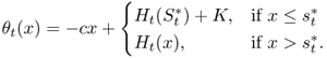
Figure 4.8 sketches ![]() and its constituent parts. The piecewise nature of
and its constituent parts. The piecewise nature of ![]() makes it nonconvex, even if
makes it nonconvex, even if ![]() is convex. Figure 4.9 plots
is convex. Figure 4.9 plots ![]() for
for ![]() for an instance with
for an instance with ![]() and
and ![]() ,
, ![]() ,
, ![]() ,
, ![]() ,
, ![]() ,
, ![]() , and
, and ![]() .
.
Fortunately, although we used convexity to prove optimality of an ![]() policy in the single‐period case, convexity is not required—an
policy in the single‐period case, convexity is not required—an ![]() policy is still optimal under a
weaker condition.
policy is still optimal under a
weaker condition.

Figure 4.8
Nonconvexity of  .
.

Figure 4.9
 for
for  ;
;  ,
,  ,
,  ,
,  ,
,  ,
,  ,
,  ,
,  .
.
Let ![]() be a real‐valued function and let
be a real‐valued function and let ![]() . Then, f is K‐convex
if, for all x and all a,
. Then, f is K‐convex
if, for all x and all a, ![]() ,
,
(Scarf, 1960). This definition is identical to (one) definition of convexity,
except for the ![]() on the right‐hand side. The term
on the right‐hand side. The term ![]() is similar to a derivative at x (think about b approaching 0). Then the left‐hand side of 4.95 approximates
is similar to a derivative at x (think about b approaching 0). Then the left‐hand side of 4.95 approximates ![]() by linearizing it using the “slope” of f between
by linearizing it using the “slope” of f between ![]() and x. (See Figure 4.10.) Therefore, K‐convexity implies that this approximation doesn't overestimate
and x. (See Figure 4.10.) Therefore, K‐convexity implies that this approximation doesn't overestimate ![]() by more than K. (It may also underestimate it.)
by more than K. (It may also underestimate it.)

Figure 4.10 K‐convexity.
If f is convex, then the approximation on the left‐hand side of 4.95
always underestimates ![]() . That is, 4.95 holds with
. That is, 4.95 holds with ![]() .
Therefore, 0‐convexity is equivalent to convexity.
.
Therefore, 0‐convexity is equivalent to convexity.
It is worth noting that, whereas some other convexity‐like properties that you may be familiar with—quasiconvexity,
pseudoconvexity, and so on—are used outside of inventory theory, K‐convexity was developed specifically for proving the optimality of ![]() policies and (as far as we know) is not used outside of inventory theory.
policies and (as far as we know) is not used outside of inventory theory.
Here is another important property of K‐convexity:
Lemma 4.16 says that a K‐convex function first decreases for a while, up to a point ![]() ; then, after a different point
; then, after a different point ![]() , if it ever decreases, it never decreases by more than K; and, in between these two points, the function never rises above its value at
, if it ever decreases, it never decreases by more than K; and, in between these two points, the function never rises above its value at ![]() . (See Figure 4.11.) This property will lead to the optimality of an
. (See Figure 4.11.) This property will lead to the optimality of an ![]() policy (as you may have suspected from our choice of notation in the lemma).
policy (as you may have suspected from our choice of notation in the lemma).

Figure 4.11 Properties of K‐convex functions from Lemma 4.16.
The following properties of K‐convex functions will be important in the results that follow. Parts (a)–(c) are generalizations of well‐known results for convexity.
Now we're finally ready to prove the optimality of ![]() policies for the finite‐horizon problem. The logic will be similar to the base‐stock case: The K‐convexity of
policies for the finite‐horizon problem. The logic will be similar to the base‐stock case: The K‐convexity of ![]() implies the K‐convexity of
implies the K‐convexity of ![]() , which implies the optimality of an
, which implies the optimality of an ![]() policy in period t and the K‐convexity of
policy in period t and the K‐convexity of ![]() ; and so on. The result was first proven by Scarf (1960); we follow the basic outline of his proof but use different arguments for some of the details.
; and so on. The result was first proven by Scarf (1960); we follow the basic outline of his proof but use different arguments for some of the details.
4.5.2.3 Infinite Horizon
If ![]() , it is still true that an
, it is still true that an ![]() policy is optimal in every period. And, echoing the infinite‐horizon model with no fixed costs, the optimal s and S are the same in every period. However, the proof of these facts is quite a bit more difficult than the analogous proof in Section 4.5.1.3, and we omit it here.
(See Zheng (1991).)
policy is optimal in every period. And, echoing the infinite‐horizon model with no fixed costs, the optimal s and S are the same in every period. However, the proof of these facts is quite a bit more difficult than the analogous proof in Section 4.5.1.3, and we omit it here.
(See Zheng (1991).)
4.6 Lost Sales
Throughout
this chapter, we have assumed that unmet demands are backordered. In this section, we assume instead that they are lost. The distinction is only important when ![]() . (When
. (When ![]() , unmet demands can only be lost.)
, unmet demands can only be lost.)
4.6.1 Zero Lead Time
In this section, we assume that the lead time
![]() . First consider the case in which
. First consider the case in which ![]() . In the finite‐horizon model, the DP recursion
4.36 changes only slightly:
. In the finite‐horizon model, the DP recursion
4.36 changes only slightly:
The only change is in the last term, where we take the positive part of ![]() to reflect the fact that the inventory level cannot become negative. A base‐stock policy is still optimal (Problem 4.44),
provided that the terminal cost
function
to reflect the fact that the inventory level cannot become negative. A base‐stock policy is still optimal (Problem 4.44),
provided that the terminal cost
function ![]() is convex
and nondecreasing. (Under backorders,
we required convexity but not monotonicity, but monotonicity is usually not a restrictive assumption under lost sales. For example, one common terminal cost function under backorders,
is convex
and nondecreasing. (Under backorders,
we required convexity but not monotonicity, but monotonicity is usually not a restrictive assumption under lost sales. For example, one common terminal cost function under backorders, ![]() , is not nondecreasing, but under lost sales,
, is not nondecreasing, but under lost sales, ![]() , and the resulting function,
, and the resulting function, ![]() is nondecreasing.) The DP algorithm
, Algorithm 4.1, applies without modification.
is nondecreasing.) The DP algorithm
, Algorithm 4.1, applies without modification.
A base‐stock policy is still optimal
for the infinite‐horizon model. Under the average‐cost criterion
(![]() ) with lost sales, it is no longer true that we order
) with lost sales, it is no longer true that we order ![]() items per period, on average, independent of the base‐stock level; therefore, we must modify the expected cost function 4.38 to account for the purchase cost. In particular, with probability
items per period, on average, independent of the base‐stock level; therefore, we must modify the expected cost function 4.38 to account for the purchase cost. In particular, with probability ![]() , we end the previous period with
, we end the previous period with ![]() and must order S units at the start of the current period; and otherwise, we must order the demand from the previous period. Therefore,
and must order S units at the start of the current period; and otherwise, we must order the demand from the previous period. Therefore,

The first‐order condition yields
The solution changes only slightly under the discounted‐cost criterion :
(In fact, 4.99 holds for the average‐cost criterion, too, setting ![]() .)
.)
When ![]() , an
, an ![]() policy is still optimal (Veinott, 1966).
In the single‐period problem, we set
policy is still optimal (Veinott, 1966).
In the single‐period problem, we set ![]() and
and ![]() as described in Section 4.4.2, unless
as described in Section 4.4.2, unless
![]() would be negative, in which case we set
would be negative, in which case we set ![]() . The finite‐horizon model (Section 4.4.3) can be modified in a manner similar to 4.96.
. The finite‐horizon model (Section 4.4.3) can be modified in a manner similar to 4.96.
4.6.2 Nonzero Lead Time
Now we allow ![]() . Recall from Section 4.3.4.1 that under backorders,
the infinite‐horizon model with
. Recall from Section 4.3.4.1 that under backorders,
the infinite‐horizon model with ![]() extends easily to nonzero lead times. Unfortunately, the same is not true under lost sales. The reason is that the logic behind the conservation‐of‐flow equation
4.41 breaks down: We can no longer subtract the entire demand in periods
extends easily to nonzero lead times. Unfortunately, the same is not true under lost sales. The reason is that the logic behind the conservation‐of‐flow equation
4.41 breaks down: We can no longer subtract the entire demand in periods ![]() because a given demand only reduces the inventory level in period
because a given demand only reduces the inventory level in period ![]() if the inventory level was sufficient when the demand occurred. The problem can be formulated as a DP
, but with an L‐dimensional state space. For reasonable values of L, the DP is typically impossible to solve exactly due to the curse of dimensionality.
Many heuristics and approximations have been proposed; see, for example, Zipkin (2008a), Bijvank and Vis (2011), or Goldberg et al. (2016) for reviews.
if the inventory level was sufficient when the demand occurred. The problem can be formulated as a DP
, but with an L‐dimensional state space. For reasonable values of L, the DP is typically impossible to solve exactly due to the curse of dimensionality.
Many heuristics and approximations have been proposed; see, for example, Zipkin (2008a), Bijvank and Vis (2011), or Goldberg et al. (2016) for reviews.
A base‐stock policy is no longer optimal (Karlin and Scarf, 1958)
for the nonzero‐lead‐time problem, and in fact the optimal policy form is unknown, aside from a few partial results about its structure—for example, that the optimal order quantity is decreasing in the on‐hand inventory (Karlin and Scarf, 1958) and that it is zero for certain vectors of on‐order inventory (Morton, 1969); Zipkin (2008b) proves these and other properties using the concept of ![]() ‐convexity
from discrete convex analysis.
‐convexity
from discrete convex analysis.
On the other hand, Huh et al. (2009) prove that a base‐stock policy is asymptotically optimal
as ![]() , and Goldberg et al. (2016) prove the asymptotic optimality as
, and Goldberg et al. (2016) prove the asymptotic optimality as ![]() of an even simpler policy in which we order the same quantity in every period.
Moreover, Levi et al. (2008) introduce a 2‐approximation algorithm
(i.e., a heuristic with a fixed worst‐case error bound of 2). Their heuristic uses a dual‐balancing policy, which means that it balances the expected marginal holding cost and the expected marginal stockout cost in each period. Order quantities in the dual‐balancing policy can be computed much more efficiently than using DP. Chen et al. (2014) present a different approximation scheme, with an (additive) error bound that can be as small as the modeler likes (but with a corresponding increase in computational complexity).
of an even simpler policy in which we order the same quantity in every period.
Moreover, Levi et al. (2008) introduce a 2‐approximation algorithm
(i.e., a heuristic with a fixed worst‐case error bound of 2). Their heuristic uses a dual‐balancing policy, which means that it balances the expected marginal holding cost and the expected marginal stockout cost in each period. Order quantities in the dual‐balancing policy can be computed much more efficiently than using DP. Chen et al. (2014) present a different approximation scheme, with an (additive) error bound that can be as small as the modeler likes (but with a corresponding increase in computational complexity).
Not surprisingly, when ![]() , the situation is even more complicated, and optimal policies are unknown for this case, too;
see, e.g., Nahmias (1979).
, the situation is even more complicated, and optimal policies are unknown for this case, too;
see, e.g., Nahmias (1979).
Lost‐sales problems with nonzero lead times are still, in many respects, an open problem and are an active area of research.
PROBLEMS
- 4.1 (Inventory of Ski Jackets) A clothing company sells ski jackets every winter but must decide in the summer how many jackets to produce. Each jacket costs $65 to produce and ship and sells for $129 at retail stores. (For the sake of simplicity, assume the jacket is sold in a single store.) Customers who wish to buy this jacket but find it out of stock will buy a competitor's jacket; in addition to the lost revenue, the company also incurs a loss‐of‐goodwill cost of $15 for each lost sale. At the end of the winter, unsold jackets are sold to a discount clothing store for $22 each.
- First suppose that the demand for the ski jackets this winter will be distributed as a normal random variable with mean 900 and standard deviation 60. What is the optimal number of jackets to produce?
- Now suppose that the demand is distributed as a Poisson random variable with mean 900. What is the optimal number of jackets to produce?
- 4.2 (Dixie's Stew) One of the specialties at Dixie's Cafe is vegetable stew, which simmers over a low flame all day. Since the cooking time is so long, Dixie must decide in the morning how many servings of the stew to cook for that night's dinner service. Moreover, the stew cooked on a given day cannot be served the next day; it must be thrown away. Vegetable stew is the highest‐profit item on the menu at Dixie's Cafe. It earns Dixie a profit of $8 per serving, whereas all the other items earn a profit of $4. Customers who want stew but find it out of stock will order one of these other items. The ingredients for one serving of stew cost the Cafe $2.50.
- First suppose that the demand for stew on a given evening is normally distributed with a mean of 18 and a variance of 16. How many servings of stew should Dixie prepare in the morning? (Fractional servings are OK.) What is the expected cost (ingredients and lost profit) of the optimal solution?
- Now suppose that the demand is distributed as an exponential random variable with mean 18. How many servings should Dixie prepare?
- 4.3 (In‐Flight Meals) Oceanic Airlines sells meals aboard their flights. Obviously, the airline must decide how many meals to put on the airplane before the flight takes off, and it cannot restock additional meals if it runs out during the flight. Each meal sells for $7 and costs the airline $2.50. If there are meals left over at the end of the flight, the perishable items must be thrown away, but nonperishable items (crackers, napkins, etc.) may be reused. The value of the reusable items is estimated at $1.50. Assume there are no loss‐of‐goodwill penalties for unmet demand, only the lost profit.
- Suppose the demand for meals on today's flight #815 has the distribution given in Table 4.3. How many meals should Oceanic stock on the flight?
- Suppose instead that the demand for meals on flight #815 has a normal distribution with mean 50 and standard deviation 10. Now how many meals should Oceanic stock?
- Calculate the optimal expected profit for meals sold on flight #815, still assuming demands are
 .
.Table 4.3 Demand for in‐flight meals for Problem 4.3. Cumulative d Probability 
Probability 
40 0.01 0.01 41 0.03 0.04 42 0.04 0.08 43 0.05 0.13 44 0.08 0.21 45 0.09 0.3 46 0.12 0.42 47 0.13 0.55 48 0.17 0.72 49 0.12 0.84 50 0.08 0.92 51 0.03 0.95 52 0.02 0.97 53 0.02 0.99 54 0.01 1
- 4.4 (Chemical Manufacturing) A chemical manufacturer produces a certain chemical compound every Sunday, which it then sells to its customers on Monday through Saturday. The company earns a revenue of $80 per kg of the compound sold. Each kg manufactured costs the company $40. If any of the compound goes unsold by Saturday night, it must be destroyed safely, at a cost of $15 per kg. The total demand for the chemical compound throughout the week has a normal distribution with a mean of 260 kg and a standard deviation of 80 kg.
- How much of the chemical compound should the company produce every Sunday?
- What is the expected cost (including manufacturing cost, lost profit, and disposal cost) per week?
- 4.5 (Cheesy Blasters) A restaurant sells a snack food called Cheesy Blasters. Cheesy Blasters are essentially nonperishable, and since they are a specialty item, customers who experience stockouts are willing to wait until a future day, i.e., their demands are backordered. Daily demand for Cheesy Blasters is distributed as
 . The restaurant orders the product from its supplier each morning. Unsold Blasters held in inventory overnight incur a holding cost of $0.75 per item, and backorders incur a penalty of $3.50 per item.
- Calculate the optimal base‐stock level and expected cost per day.
- Assuming the restaurant uses the base‐stock level from part (a), calculate its type‐1 and type‐2 service levels. For type‐2, calculate its exact service level, B, and both approximate service levels,
 and
and  .
. - Repeat part (b) assuming that the restaurant uses a base‐stock level of 30.
- Now assume that the restaurant can only place a replenishment order once per week (7 days), and that the supply lead time is 2 days. Calculate the optimal base‐stock level and expected cost per period.
- Repeat part (b) for the system described in part (d), using the optimal base‐stock level.
- 4.6 (Electricity Generation) On
day t, an electricity utility company must decide how much generation capacity to prepare for the electricity it will generate on day
 . Each megawatt‐hour (MWh) of capacity prepared costs the utility r. Let
  be the generation capacity chosen on day t for generation on day
  .
.The demand for day
 , denoted
  , is stochastic, with pdf
  and cdf
  .
.  is not observed until day
  , although for simplicity we will assume that the entire day's demand is revealed at the beginning of the day.
Once
 is observed, the utility generates
  MWh of electricity. Each MWh of electricity actually generated incurs a cost of c per MWh (in addition to the cost r already incurred to prepare the capacity). If
  , the utility must purchase electricity on the spot market to make up the difference. (The spot market is a marketplace in which the utility can purchase an unlimited quantity of electricity with no advance notice required.) The price per MWh of electricity purchased on the spot market is m, with
  .
.- Write an expression for
 , the optimal number of MWh of capacity to prepare.
 - Suppose
r = $5/MWh, c = $2/MWh, m = $20/MWh, and
 MWh. What is
  ?
?
- Write an expression for
- 4.7 (Newsvendor Applications #1) Each of the situations below can be interpreted as a newsvendor problem. For each, indicate the holding and stockout costs, h and p, and use the results of Section 4.3.2 to find
 .
.- You are about to sign a 2‐year contract for a mobile phone and you need to decide how many minutes per month to commit to purchasing. You can purchase any number S of minutes. (You are not restricted to rate plans specified by your mobile phone company.) If you commit to purchasing S minutes per month, you pay $0.05 for each of these S minutes (regardless of whether or not you use them), plus $0.25 for each minute you use in excess of S.
(For example, if
 and you use 120 minutes, you pay
  .)
.)Your monthly usage of minutes has a normal distribution with mean 1000 and standard deviation 220.
- You are the producer of a new TV show and are about to negotiate a contract with the star of the show. You need to decide how many seasons (years) to commit to in the contract, but you are not sure how many seasons of the show will be produced before it is canceled. For each season you commit to in the contract, the star's salary will be $1.5 million. If you commit to S years but the show lasts for longer than that, you will have to pay the star $2.5 million per season (since she will become more popular in the future and will demand a higher salary). If you commit to S years but the show is canceled earlier than that, you do not need to pay the star's salary for seasons that were not produced; instead, you must pay her a $500,000 contract‐cancellation fee for each season committed to but not produced.
(For example, if you commit to 3 seasons and the show is produced for 4 seasons, you will pay $1.5 × 3 + $2.5 × 1 = $7 million. If the show is produced for 2 seasons, you will pay $1.5 × 2 + $0.5 × 1 = $3.5 million.)
Table 4.4 lists your estimates that the show will last for exactly x seasons, for various values of x.
Table 4.4 Probability distribution of TV show duration for Problem 4.7(b).
x 
1 0.25 2 0.05 3 0.10 4 0.20 5 0.15 6 0.10 7 0.10 8 0.05 - You are purchasing tickets for a group of students to attend a minor league baseball game. Tickets cost $8 each when purchased in advance. The number of students who will actually show up to the game is random and has a Poisson distribution with mean 26. Suppose you purchase S tickets. If fewer than S students show up for the game, you can return the extra tickets to the box office for half of their original price. If more than S students show up for the game, you will need to buy tickets from “scalpers” (people selling tickets outside the stadium) for $30 each.
- You are about to sign a 2‐year contract for a mobile phone and you need to decide how many minutes per month to commit to purchasing. You can purchase any number S of minutes. (You are not restricted to rate plans specified by your mobile phone company.) If you commit to purchasing S minutes per month, you pay $0.05 for each of these S minutes (regardless of whether or not you use them), plus $0.25 for each minute you use in excess of S.
- 4.8 (Newsvendor Applications #2) Follow the instructions for Problem 4.7 for each of the following situations.
- You are the manager of an auto‐repair shop at which every car requires the entire day to repair. The shop does not accept appointments; customers arrive randomly. All customers arrive exactly when the shop opens in the morning.
If the number of auto mechanics on duty on a given day, S, is at least as large as the number of customers that arrive in the morning, all of the customers' cars will be repaired. If the number of customers exceeds S, however, the extra customers leave and get their car repaired at a competing shop across the street.
The number of customers arriving in a given day has a Poisson distribution with a mean of 18. Each car that is repaired earns the shop a profit of $470, and each mechanic on duty costs the shop $200 per day.
- At the beginning of the academic year, you need to decide how many “dining dollars” to put on your university ID card. Dining dollars earn you a 15% discount on the food you buy on campus—so $100 in dining dollars buys you
 in food. However, any dining dollars not spent by the end of the academic year are lost. (Yes—you could just stock up on soda and potato chips at the end of the year to spend your remaining dollars. But pretend that's not possible.) The (undiscounted) value of the food you buy in 1 year is given by the random variable X, which has a lognormal distribution
with parameters
in food. However, any dining dollars not spent by the end of the academic year are lost. (Yes—you could just stock up on soda and potato chips at the end of the year to spend your remaining dollars. But pretend that's not possible.) The (undiscounted) value of the food you buy in 1 year is given by the random variable X, which has a lognormal distribution
with parameters  and scale parameter
  . (That is,
  has a normal distribution with mean 6 and standard deviation 0.3.)
 - A small cement manufacturer operates a single truck, which makes deliveries throughout the day. The company must decide how much cement to load onto the truck each morning, before knowing how much cement each customer will request. It costs the company $20 per cubic yard loaded onto the truck, in materials and labor costs. For each cubic yard of cement sold, the company earns $65 in profit. The total demand for cement in a given day (summed over all the firm's customers) is normally distributed with a mean of 7 cubic yards and a standard deviation of 3 cubic yards.
There is no opportunity to load more cement for the rest of the day. Any unused cement at the end of the day must be discarded, with no salvage value—in fact, it costs the company $35 per cubic yard in labor to clean out the dried‐up cement from the truck. Assume the truck's capacity is large enough to hold any desired amount of cement.
- You are the manager of an auto‐repair shop at which every car requires the entire day to repair. The shop does not accept appointments; customers arrive randomly. All customers arrive exactly when the shop opens in the morning.
- 4.9 (Simulation of Mobile‐Phone Contract) Simulate the system in Problem 4.7(a) for 1000 months in a spreadsheet program. For each month, generate a random variate from the appropriate distribution and calculate the resulting cost. In your writeup, include the first 10 rows of your spreadsheet and report the average total cost per month (including the cost of the contracted minutes).
- 4.10 (Simulation of Dining Dollars) Simulate the system in Problem 4.8(b) for 1000 years in a spreadsheet program. For each year, generate a random variate from the appropriate distribution and calculate the resulting cost. In your writeup, include the first 10 rows of your spreadsheet and report the average total overage and underage cost per year.
- 4.11 (Managing Blood Inventory) A hospital purchases blood from a local blood‐donation organization and uses it for patients during surgeries and emergency procedures. The hospital pays $175 for each unit of blood purchased. Orders must be placed first thing in the morning, and any blood not used by the end of the day must be discarded. There is no salvage value or cost to discard a unit of blood. If the hospital needs more blood on a given day than they purchased that morning, they must place an emergency order; blood ordered this way costs $420 instead of $175. The number of units of blood that the hospital uses on a given day is normally distributed, with a mean of 150 and a standard deviation of 40.
- Interpret this problem as a newsvendor problem. What are the holding and stockout costs, h and p?
- What is the optimal number of units of blood for the hospital to purchase in the morning? (Fractional answers are OK.)
- On what fraction of days will the hospital need to order at least one emergency unit of blood?
- Suppose unused inventory costs the hospital money to dispose. Will the optimal order quantity increase, decrease, or stay the same? Will the optimal expected cost increase, decrease, or stay the same?
- 4.12 (Inventory Simulation) Using
a spreadsheet software package of your choice, simulate an infinite‐horizon base‐stock policy (Section 4.3.4
). Your spreadsheet should include columns for the starting and ending inventory level; the order quantity; the random demand; and the total cost (as well as any other columns you wish to include). Use the optimal base‐stock level S (which should be calculated within your spreadsheet) and assume that the system begins period 1 with S units on hand.
- Assume that demands per period are
 and that
  ,
,  ,
,  , and
, and  . Simulate the system for at least 1000 periods and include the first 10 rows of your spreadsheet in your report.
 - For each performance measure listed below, calculate the exact mean value (using formulas contained in this chapter) and the mean value from the simulation, and compare the two.
- Ending inventory level
- Order quantity
- Holding cost per period
- Stockout cost per period
- Total cost per period
- Type‐1 service level
- Type‐2 service level
- Assume that demands per period are
- 4.13 (Inventory Simulation: Fixed Cost) Add
a fixed ordering cost K to your simulation from Problem 4.12 and implement an
 inventory policy. Calculate optimal, or near‐optimal, values of the policy parameters s and S in the spreadsheet and use those for the simulation. Assume
  . Report the simulated mean values for each of the performance measure listed in Problem 4.12(b). (Make sure to include the fixed cost when you report the total cost.)
 - 4.14 (Inventory Simulation: Lead Time) Modify
your simulation from Problem 4.12 to handle a nonzero lead time L. Calculate the optimal value of S in the spreadsheet and use it for the simulation. Assume
 . Report the simulated mean values for each of the performance measures listed
in Problem 4.12(b).
. Report the simulated mean values for each of the performance measures listed
in Problem 4.12(b). - 4.15 (Implicit vs. Explicit Newsvendor Cost Functions) Let
 and
and  . Prove that the (implicit) newsvendor cost function 4.12 under cost parameters
  and
and  is equal to the explicit newsvendor cost function 4.19 plus the constant
  , which represents the expected margin earned on the units
sold.
, which represents the expected margin earned on the units
sold. - 4.16 (Discrete Newsvendor with Continuous Demands) Suppose
that the newsvendor's demand has a continuous distribution but the newsvendor must choose integer values of S. Prove (by giving examples) that
 can equal either
 or S, where S is such that
  .
. - 4.17 (Alternate Fill Rate Formula) Silver and Bischak (2011) prove
the following formula for the type‐2 service level under an infinite‐horizon base‐stock policy with lead time
 and reorder interval
  :
:
where
 is the coefficient of variation for the demand in one period and
- 4.18 (Newsvendor with Forecasting) Suppose that demands are normally distributed and that the newsvendor does not know
 and
and  , but he estimates them in each period, as described in Section 4.3.2.7, using moving averages and standard deviations with
  . The observed demands in periods
  are 99, 87, 125, 106, 100, 107, 93, 114, 87, and 85. The cost parameters are
  and
and  . What is the optimal order quantity for the newsvendor in period t?
 - 4.19 (Lognormal Newsvendor) Suppose
the demand D has a lognormal distribution
with parameters
 and
and  . (That is,
  .) Prove that the optimal solution to the newsvendor problem and its expected cost are given by
where
 .
.Hint: The loss function for the lognormal distribution for
 is(4.102)
- 4.20 (The Cooperative Newsvendor) Consider
a newsvendor who purchases newspapers from his supplier at a cost of c per newspaper and sells them at a price of r per newspaper. If he has unsold newspapers at the end of the day, he can take them to the local recycling center, which pays him a salvage value of v per newspaper. The daily demand for newspapers has pdf
 and cdf
  . Assume that
  is strictly increasing.
- Write the newsvendor's expected cost as a function of S, denoted
 . (Your expression may include integrals.) Show that the order quantity that minimizes
  is
is
- Suppose the newsvendor's supplier prints newspapers on demand; that is, she observes the newsvendor's order of S and then prints exactly S newspapers. The supplier therefore faces no uncertainty. It costs the supplier b to print one newspaper. Write the supplier's expected net cost (i.e., cost minus revenue) as a function of S, denoted
 . Then write the total supply chain expected cost as a function of S, denoted
  —that is,
  .
. - Find the order quantity
 that minimizes
  . (If the supplier and the newsvendor were both owned by a single firm that sought to minimize its total costs, this is the order quantity it would pick.)
 - Prove that
 if and only if
  —that is, if and only if the supplier earns zero profit on each newspaper she sells to the newsvendor.
 - Prove that
 if and only if
  , and
, and  otherwise.
 - In a short paragraph, discuss the implications of the results you proved in this problem. What does it mean for two supply chain partners that are each attempting to minimize their own costs rather than minimizing the total supply chain cost?
- Write the newsvendor's expected cost as a function of S, denoted
- 4.21 (
 for Poisson Newsvendor) Suppose that in the newsvendor problem, the demand per period, D, has a Poisson distribution
with mean
for Poisson Newsvendor) Suppose that in the newsvendor problem, the demand per period, D, has a Poisson distribution
with mean  . Suppose further that there exists an
  such that
  . Prove that
- 4.22 (Non‐Standard‐Normal Loss Function) Prove equation 4.25 (also given in (C.31)).
- 4.23 (Loss Function Derivatives) Prove equations 4.13 and 4.14 (also given in (C.15) and (C.16)).
- 4.24 (Uniform Loss Functions)
Derive expressions for the first‐ and second‐order loss and complementary loss functions for the continuous
 distribution.
 - 4.25 (A Simple Revenue Management Problem) An
airplane has n seats in coach class. Two types of travelers will purchase tickets for a certain flight on a certain date: leisure travelers, who are willing to pay only the discounted fare
 , and business travelers, who are willing to pay the full fare
 (
( ). The airline knows that the number of leisure travelers requesting tickets for this flight will be greater than n for sure, while the number of business travelers requesting tickets is a random variable X with a given cdf
  .
.Assume that the leisure travelers always purchase their tickets before the business travelers do. (In practice, this is roughly true, which is why airfares increase as the flight date gets closer.) The airline wishes to sell as many seats as possible to business travelers since they are willing to pay more. However, since the number of such travelers is random and these customers arrive near the date of the flight, a sensible strategy is for the airline to allocate a certain number of seats Q for full fares and the remainder,
 , for discount fares.
The discount fares are sold first: The first
 customers requesting tickets will be charged
  , and the remaining
  Q customers will be offered the full price
  . Some of the customers being offered
  will be leisure travelers; these travelers will decline to buy a ticket. Similarly, it is possible that some of the seats sold to leisure travelers for
  could have been sold to business travelers who would have been willing to pay
  .
.- Show that the problem of finding the optimal number of full‐fare seats, Q, is equivalent to a newsvendor problem. What should be used in place of the holding and stockout costs h and p? What is the critical ratio? What is the optimality condition (analogous to 4.16)?
- Suppose that demand for full‐fare seats is normally distributed with a mean of 40 and a standard deviation of 18. There are
 seats on the flight, and the fares are
  $189 and
  $439. What is the optimal number of full‐fare seats? (Fractional solutions are OK.)
 - For each of the following situations, will the optimal Q increase, decrease, or stay the same? Will the optimal cost increase, decrease, or stay the same? Briefly explain your answers.
- The full‐fare tickets are fully refundable, and with some probability each business traveler will cancel his or her ticket at the last minute, too late for the airline to resell the newly vacant seat.
- A fraction of leisure travelers are willing to pay full fare if they arrive after the discount seats are sold out.
- Unsold seats may be sold at the very last minute for a steeply discounted price (for example, on a discount airfare website). These tickets are made available after most (though not necessarily all) of the business travelers have requested tickets.
- 4.26 (Allocating Parking Spots) You are the manager of a luxury apartment building whose parking garage contains 300 parking spots. Residents may choose to purchase a dedicated parking spot for $60,000 for 3 years. (Only 3‐year contracts are available.) The garage also has metered parking spots that require drivers to pay $4 per hour for parking. The number of drivers wishing to park in metered spots in a given hour has a normal distribution with a mean of 50 and a standard deviation of 10. Your goal is to choose how to allocate the 300 spots between dedicated and metered spots.
To keep things simple, assume that (1) the demand for dedicated spots is greater than 300; (2) drivers who park in metered spots all park for exactly 1 hour, arriving and departing on the hour (at 12:00, 1:00, etc.); and drivers who purchase dedicated spots never park in metered spots, and vice‐versa.
What is the optimal number of spots to designate as metered spots?
- 4.27 (Free Overage) Suppose that, in the newsvendor problem, we are allowed up to r units of overage for free before incurring holding costs, where
 is a constant. That is, the cost if we order S units and have a demand of d is
  .
.
- 4.28 (DP Walkthrough) The demand for a given product in each period equals 2 with probability 0.2, 1 with probability 0.5, and 0 with probability 0.3. Holding and stockout costs per period are given by
 and
and  . The purchase cost is
  , and there is no fixed cost. The order‐up‐to level y in each period must be in
  . The planning horizon is
  periods, and the terminal cost at the end of the horizon is given by
  . We begin period 1 with
  units on hand. Using Algorithm 4.1, determine
  for
for  and for each feasible value of x. Also determine the expected cost for the entire horizon (including the terminal cost), given that we begin the horizon with
  . Work through the algorithm by hand and show your work.
 - 4.29 (Implementing Base‐Stock DP) Consider
the finite‐horizon model with no fixed costs of Section 4.3.3.
- Implement the DP model in any programming language you wish.
- Suppose
 ,
,  ,
,  ,
,  , and
, and  . Suppose the demand per period is distributed as
  and the terminal cost function is given by
where
 and
and  . Using your DP, find
  and
and  for
for  and
and  . Report these in two separate tables. Also report the optimal base‐stock level
  for periods
  .
. - Plot
 for
for  .
.
- 4.30 (Implementing
 DP) Consider
the finite‐horizon model with fixed costs of Section 4.4.3.
DP) Consider
the finite‐horizon model with fixed costs of Section 4.4.3.- Implement the DP model in any programming language you wish.
- Suppose
 ,
,  ,
,  ,
,  ,
,  , and
, and  . Suppose the demand per period is distributed as
  and the terminal cost function is given by
where
 and
and  . Using your DP, find
  and
and  for
for  and
and  . Report these in two separate tables. Also report the optimal parameters
  and
and  for periods
  .
. - Plot
 for
for  .
.
- 4.31 (
 for Refrigerators) Weekly
demand for refrigerators at an appliance store has a Poisson distribution with a mean of 4. The holding and stockout cost for refrigerators at the store are h = $40 and p = $125 per week, respectively. Replenishment orders for refrigerators incur a fixed cost of K = $150.
for Refrigerators) Weekly
demand for refrigerators at an appliance store has a Poisson distribution with a mean of 4. The holding and stockout cost for refrigerators at the store are h = $40 and p = $125 per week, respectively. Replenishment orders for refrigerators incur a fixed cost of K = $150.- Suppose we set
 . What is the expected cost per week?
 - Using Algorithm 4.2, find the optimal parameters
 , and the corresponding optimal cost.
- Suppose we set
- 4.32 (Approximate
 Policies) Consider an infinite‐horizon instance in which the demand per period is normally distributed with a mean of 190 and a standard deviation of 48, and in which the costs are given by
  ,
,  , and
, and  . Determine approximate values for s and S:
- Using the
 approximation.
 - Using the power approximation.
- Using the
- 4.33 (Ordering Capacities)
Suppose that an ordering capacity of b units is imposed in the finite‐horizon model with no fixed costs of Section 4.3.3. Sketch a plot of
 vs. x, analogous to Figure 4.4. (The exact numbers are not important; what is important is the shape of the curve.)
 - 4.34 (DP for Ordering Capacities)
Suppose that an ordering capacity of b units is imposed in the finite‐horizon model with fixed costs of Section 4.4.3.
- Explain how to modify the DP from Section 4.4.3 to account for the ordering capacity.
- Implement your DP from part (a). Using your DP, find
 and
and  for
for  and
and  for the instance described in Problem 4.30(b) using a capacity of
  . Report
  and
and  in two separate tables.
- 4.35 (Nonoptimality of
 Policies for Ordering Capacities) Suppose that an ordering capacity of b units is imposed in the finite‐horizon model with fixed costs of Section 4.4.3. Prove, by providing a counter‐example, that an
  policy is not necessarily optimal in every period of the finite‐horizon version of this problem. (The
  policy is modified in this case: If
  , we order
  , and otherwise, we order nothing, where
  is the current inventory
position.)
is the current inventory
position.) - 4.36 (K‐Convexity Is Not a Necessary Condition)
In Section 4.5.2.2, we proved that if
 is continuous and K‐convex, then an
  policy is optimal in period t. However, K‐convexity is not a necessary condition: An
  policy can still be optimal in period t even if
  is not K‐convex. Sketch a graph of a function
  that is not K‐convex but for which an
  policy is optimal. Explain clearly (a) why the function is not K‐convex and (b) why an
  policy is optimal.
 - 4.37 (Other Policy Forms #1) Consider the single‐period model with no fixed costs from Section 4.5.1.1. We know that, for a given starting inventory level x, 4.83 determines the optimal inventory position after ordering, y. We assumed a particular form for
 and used the convexity of this function to prove the optimality of a base‐stock policy. But in principle
  can have any form, and other policies may be optimal for other functions.
- Develop a function
 such that the optimal policy has three parameters,
  ,
,  , and
, and  (
( ), and has the following form:
- If
 , then order up to
  .
. - If
 , do nothing.
 - If
 , order up to
  .
. - If
 , do nothing.
For the sake of simplicity, assume that
 . Sketch the function
  and explain how to determine the optimal values of the parameters
  ,
,  , and
, and  . (For example, “
 is the largest maximizer of
  .”)
.”) - If
- Now suppose that
 so that the term
  is now added to the objective function, as in 4.92. Develop a function
  such that the optimal policy has four parameters,
  ,
,  ,
,  , and
, and  (
( ), and has the following form:
- If
 , then order up to
  .
. - If
 , do nothing.
 - If
 , order up to
  .
. - If
 , do nothing.
Sketch the function
 and explain how to determine the optimal values of the parameters
  ,
,  ,
,  , and
, and  .
. - If
- Develop a function
- 4.38 (Other Policy Forms #2) Describe the form of the optimal single‐period inventory policy for each of the functions
 depicted in Figure 4.14 (in a manner similar to the descriptions in Problem 4.37). Explain how to determine the optimal values of the parameters for your policy. Note that in part (c), there is a fixed cost of K, and in part (c), there is an ordering capacity of b units. For all parts, assume that the per‐unit cost
  .
. 
Figure 4.14
 functions for Problem 4.38, with fixed cost
  and ordering capacity
  .
. - 4.39 (Other Policy Forms #3) Suppose that, in the single‐period model with fixed costs of Section 4.5.2.1, the function
 has a shape similar to the curve in Figure 4.15, with
  .
.- Prove that
 is not K‐convex.
 - Describe the form of the optimal inventory policy (in a manner similar to the descriptions in Problem 4.37). Explain how to determine the optimal values of the parameters for your policy.
- Write a set of conditions on
 that ensures that, if all of your conditions hold, then the policy that you described in part (b) is optimal. Your conditions must be sufficient but need not be necessary.
Figure 4.15  function for Problem 4.39, with fixed cost
  .
.
- Prove that
- 4.40 (Single‐Period Control‐Band Policies)
Consider the single‐period model without fixed costs of Section 4.5.1.1, and suppose we begin the period with an inventory level of
 . Suppose further that we can return excess inventory to the supplier in each period. That is, we can choose
  , or equivalently,
  .
.For each unit we return, we earn a revenue of
 , so the total revenue earned when
  is
is  . Normally
  , but it's also possible that
  , in which case we pay a cost to make the return.
Consider the following policy: There are two parameters, S and U, with
 . Set
. Set
The interval
 is called a control band, and the policy is called a control‐band policy. The idea is to order up to S if x is below the control band, to “return down to” U if x is above the control band, and to do nothing if x is in the control band.
- Prove that a control‐band policy is optimal for the single‐period problem.
- Show how to calculate the optimal
 and
and  for the single‐period problem, and prove that
  .
. - Prove that, in the single‐period problem, as
 (from above),
  . In a few sentences, explain why it is logical to require
  .
. - Prove that, in the single‐period problem, as
 (from below),
  . In a few sentences, explain why it is logical to require
  .
. - Suppose the demand per period is distributed as
 . Suppose
  ,
,  ,
,  , and
, and  . Find
  and
and  for the single‐period problem.
- 4.41 (Finite‐Horizon Control‐Band Policies) Return to the setup in Problem 4.40, and now consider the finite‐horizon model. Prove that a control‐band policy is optimal in every period of the finite‐horizon model. (The parameters of the control‐band policy are now indexed by
time,
 and
and  .)
.) - 4.42 (Properties of K‐Convex Functions) Prove Lemma 4.17.
- 4.43 (Alternate Terminal Cost Function)
Consider the finite‐horizon base‐stock model described in Section 4.5.1.2. Suppose that the terminal cost function is given by(4.103)

Suppose also that
 .
.- Write an expression for
 .
. - Derive the optimal base‐stock level in period T, in the form

- Write an expression for
 . (Note: Your expression may involve cases, as in 4.90.)
 - Derive the optimal base‐stock level in period
 , in the form
- Prove
that
 .
.
- Write an expression for
- 4.44 (Finite‐Horizon Base‐Stock Policies under Lost Sales)
Prove that, if the terminal cost function
 is convex and
  , then a base‐stock policy is optimal in each period of the finite‐horizon problem with no fixed costs under lost sales. (The condition
  essentially ensures that the condition
  continues to hold even in the terminal cost function.)
 - 4.45 (Minimum Order Quantity)
Consider the single‐period model without fixed costs from Sections 4.3.2 and 4.5.1. Suppose there is a constraint requiring the order quantity to be either 0 or at least M, where
 is a constant.
- One plausible policy for this problem is a modified base‐stock policy in which we order
 , where x is the starting inventory level. Prove (by giving a counterexample) that this policy is not optimal.
 - Another plausible policy is an
 policy in which
  . Prove that this policy is not optimal either.
 - Make a conjecture as to the form of the optimal policy. (That is, describe a decision rule, similar to how we described the policies in Section 4.1.)
- Bonus: Specify the optimal parameters of the policy you described in part (c).
- Double Bonus: Prove that the policy you described in parts (c) and (d) is optimal.
- One plausible policy for this problem is a modified base‐stock policy in which we order
- 4.46 (Monotonic Safety Stock) Consider the infinite‐horizon base‐stock model with service‐level constraints given by 4.62–4.64.
- Suppose we use a type‐1 service‐level constraint 4.63. Argue that the optimal base‐stock level and the optimal safety‐stock level (given by the optimal base‐stock level minus the mean lead‐time demand,
 ) both increase as the reorder interval R increases.
 - Suppose we use a type‐2 service‐level constraint 4.64 under approximation
 . Argue that the optimal base‐stock level increases as R increases, but show that the optimal safety‐stock level can decrease as R increases.
- Suppose we use a type‐1 service‐level constraint 4.63. Argue that the optimal base‐stock level and the optimal safety‐stock level (given by the optimal base‐stock level minus the mean lead‐time demand,
- 4.47 (Derivatives of
 and
and
 ) Assuming the demand is distributed
  , prove that
where
 and
and  are as defined in Section 4.3.2.2 and
  .
. - 4.48 (DP for New and Used Items) A company manufactures and sells a laptop computer that has a market both for new items and for used ones. In each period, the firm decides how much to manufacture and then observes the demand for each type (new and used). Demand is satisfied as much as possible, and then a portion of the unused new inventory “expires” and is considered used. Unmet demand for new products is backordered but unmet demand for used products is lost. Products cannot be substituted; that is, a customer demanding a used item cannot be given a new item, and vice‐versa.
Use subscript 1 to denote new items and subscript 2 to denote used items. Thus, the holding and stockout costs per item per period for new items are given by
 and
and  , respectively. For used items, the holding cost per item per period is given by
  , and the stockout cost per item is given by
  . Assume that demands of type i (
 ) are independent and normally distributed with pdf
  and that the demand for each type in a given period is independent of the demand for the other type. There is no fixed ordering cost, and the discount factor is
  .
.The sequence of events in each time period is as follows:
- The inventory levels
 and
and  of new and used items (respectively) are observed.
 - A manufacturing order for new items is placed and is ready instantaneously.
- Demands
 and
and  for new and used items (respectively) are observed. As much demand as possible is satisfied from the two inventories. Unmet demands for new items are backordered and unmet demands for used items are lost.
 -
 new items are transferred to the used inventory, where
  is a constant (
 ) and
) and  is the inventory level of new items after the manufacturing order is received and the demand is subtracted, i.e., after step 3.
 - Holding and stockout costs are assessed based on the ending on‐hand inventory levels.
Let
 be the optimal expected cost in periods
  if we begin period t with a new‐item inventory level of
  and a used‐item inventory level of
  (and act optimally thereafter). Formulate a recursive (DP) expression for
  , analogous to 4.36.
Your expression must use y, the order‐up‐to level for new items, as the decision variable for the minimization. Do not write the expectation as
 . Instead, write out the expectation using integrals. If you define any additional notation, define it clearly.
 - The inventory levels
