
Chapter 30
Case Study, Part 2: Clustering and Principal Components Analysis
Chapters 29–32 present a Case Study of Predicting Response to Direct-Mail Marketing. In Chapter 29, we opened our Case Study with a look at the primary and secondary objectives of the project, which are reprised here.
- Primary objective: Develop a classification model that will maximize profits for direct-mail marketing.
- Secondary objective: Develop better understanding of our clientele through exploratory data analysis (EDA), component profiles, and cluster profiles.
The EDA performed in Chapter 29 allowed us to learn some interesting customer behaviors. Here in this chapter, we learn more about our customers through the use of principal components analysis (PCA) and clustering analysis. In Chapter 31, we tackle our primary objective of developing a profitable classification model.
30.1 Partitioning the Data
The analyses we perform in Chapters 29–31 require cross-validation. We therefore partition the data set into a Case Study Training Data Set and a Case Study Test Data Set. The data miner decides the proportional size of the training and test sets, with typical sizes usually ranging from 50% training/50% test to 90% training/10% test. In this Case Study, we choose a partition of approximately 75% training and 25% test.
30.1.1 Validating the Partition
In Chapter 6, we discussed methods for validating that our partition of the data set is random, using some simple tests of hypothesis. However, such methods may become tedious when testing for dozens of predictors. Equivalent computational methods exist for performing these tests on a large set of predictors. Figure 30.1 shows the results of F-tests (equivalent to t-tests in this case) performed on some of the continuous variables in our Case Study. (In Modeler, use the append node to put the training and test data sets together, then use the means node to examine for difference in means, based on the source input.) The null hypothesis is that there is no difference in means; the Importance field equals 1 − p-value. None of the fields was found to be significant. Remember, that we might expect on average about 1 out of 20 tests to be significant, even if there is no difference in means.
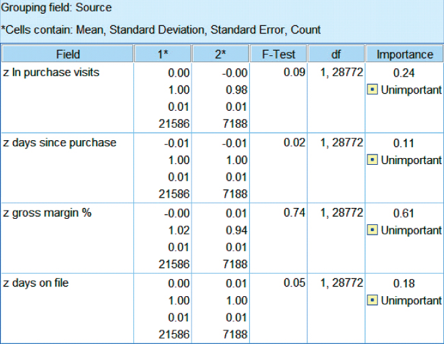
Figure 30.1 No significant difference in means for continuous variables.
Investigation of some noncontinuous variables (not shown) indicates no systematic deviations from randomness. We thus conclude that the partition is sound, and proceed with our analysis.
30.2 Developing the Principal Components
PCA is useful when using models such as multiple regression or logistic regression, which become unstable when the predictors are highly correlated. However, PCA is also useful for uncovering natural affinities among groups of predictors, which may be of interest to the client. In other words, PCA is useful both for downstream modeling, and for its component profiles.
Figure 30.2 shows the variables input to our PCA. Note that all variables are continuous, and so do not include the flag or nominal variables, because PCA requires continuous predictors. Also, of course, the response variable is not included.
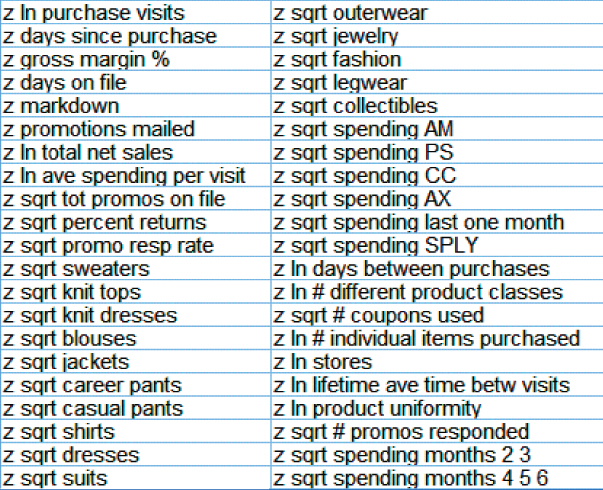
Figure 30.2 Predictors input to PCA.
PCA is applied to the training data set using these inputs, with minimum eigenvalue = 1.0, and using varimax rotation. The rotated results shown in Figure 30.3 show that 13 components were extracted, for a total variance explained of 68.591%.
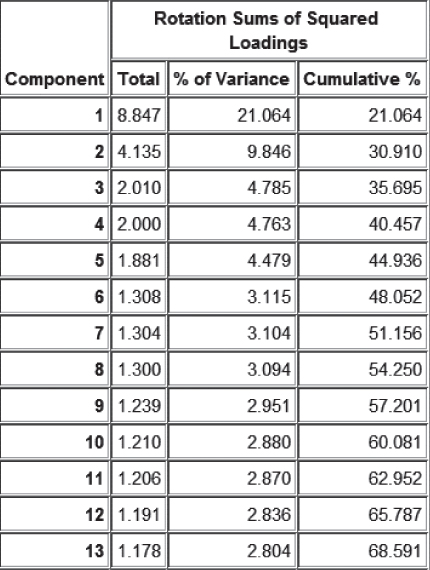
Figure 30.3 Results from PCA to all continuous predictors.
Unfortunately, it turns out that the communalities for several of the predictors are rather low (<0.5, output not shown), given in Table 30.1. Low communalities mean that these variables share little variability in common with the set of other predictors. Thus, it makes sense to remove them as inputs from the PCA, and try again. PCA is again applied to the training data set, this time without the set of eight predictors from Table 30.1, using the same settings as previously. This time, Figure 30.4 shows that only 11 components are extracted, for a total variance explained of 75.115%.
Table 30.1 Set of predictors with low communality, that is, which do not share much variability with the remaining predictors
| z sqrt knit tops | z sqrt dresses |
| z sqrt jewelry | z sqrt fashion |
| z sqrt legwear | z sqrt spending AX |
| z sqrt spending SPLY | z sqrt spending last one month |
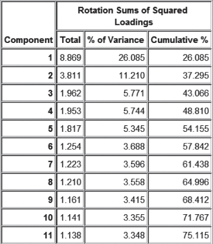
Figure 30.4 Eliminating low communality predictors reduced number of components and increased variance explained.
Unfortunately, at this point, z sqrt spending AM exhibits relatively low communality (0.470) with the remaining predictors, a behavior reflected in both the training and test sets (not shown). This variable is therefore set aside, and PCA analysis is applied to the reduced set of predictors (omitting the eight in Table 30.1 and z sqrt spending AM). The results for the training set are shown in Figure 30.5. Eliminating another predictor from the PCA has again increased the cumulative variance explained, although this may be, in part, because omitting this variable has reduced the overall amount of variability to explain.
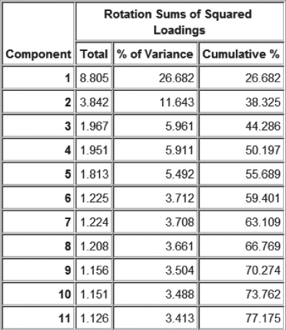
Figure 30.5 Eliminating another predictor from the PCA has again increased the variance explained.
Before we move forward with this PCA solution, what is to become of the predictors that were omitted from the PCA model? As they have little correlation with the other predictors, they are to move on to the modeling stage without being subsumed into the principal components. PCA analysis of these nine predictors shows that, even among themselves, there is little correlation (Figure 30.6, for the training set). Further, only two components were extracted from this set of eight predictors, with less than 30% of the variance explained (not shown). Thus, these nine variables are free to move on to the modeling stage without the need for PCA. However, they will not contribute to the knowledge of our customer database that we will uncover using profiles of the principal components.

Figure 30.6 Little variance in common among the predictors not partaking in the PCA.
We therefore proceed with the PCA of all continuous predictors, except those in Figure 30.6.
30.3 Validating the Principal Components
Just as with any modeling procedure, the analyst should validate the PCA, using cross-validation. Figure 30.7 contains the rotated component matrix for the training data set, showing which variables belong to which component. Values smaller than 0.5 are suppressed, to enhance interpretability. Compare with Figure 30.8, which shows the rotated component matrix for the test data set. The components are broadly similar between the training and test sets, with some minor differences. For example, the test set shows that z sqrt spending PS belongs to Component 1, while the training set disagrees. However, the test set component weight is only 0.502, barely above the 0.5 cutoff for suppression. So, we read this as good news for Component 1, because the training and test sets agree on all variables except this z sqrt spending PS, which may considered of dubious membership to Component 1.

Figure 30.7 Rotated component matrix (training data set), showing which variables belong to which component.

Figure 30.8 Rotated component matrix for the test data set.
Other minor differences between the training and test sets include the following. The component weights are not equal, but this is to be expected due to random noise. Components 3 and 4 are mischievously switched by the test data set, but retain their essence. However, broadly speaking, there is good agreement between the components extracted from the training and test data sets. We conclude therefore that our PCA is validated.
30.4 Profiling the Principal Components
Apart from their use to mitigate multicollinearity for downstream modeling, principal components are most useful for learning about how the variables interact. In fact, the analyst should always provide descriptive profiles of the principal components, both as a reality check for the analyst, as well as to enhance the client's understanding. The analyst should ask, “Do these principal components (which are mathematical entities, after all) correspond to identifiable real-world commonsense behaviors?” If there is a problem with interpretability, then this may indicate some computational or procedural error upstream. If the principal components do correspond to real-world behaviors, then this acts as further validation of their “reality,” as well as providing useful information for the client.
To profile the components, we will work with the rotated component matrix generated by training set (Figure 30.7), which leveraged more records than the test set. Note that Component 1 is a large and complex component, consisting of many predictors, with both positive and negative component weights. This is often the case in PCA, with the first component often representing a general type of phenomenon such as “size,” or “sales.” In fact, without the varimax rotation, the first component would have been even larger. Table 30.2 indicates the positive and negative weighted predictors in Component 1.
Table 30.2 Predictors with positive and negative weights in Component 1 (“z ln” and “z sqrt” suppressed for clarity)
| Positive Component Weight | Negative Component Weight |
| # Individual items purchased | Days between purchases |
| Purchase visits | Lifetime average time between visits |
| Total net sales | Days since purchase |
| # Different product classes | Product uniformity |
| Spending months 4 5 6 | |
| # Coupons used | |
| Stores | |
| Promo response rate | |
| Spending months 2 3 | |
| # Promos responded | |
| Spending at CC store |
We would describe Component 1 as measuring “Sales Volume and Frequency.” This component measures sales volume and frequency in many ways, which are as follows:
- How many items are purchased?
- How often does the customer visit?
- How long does the customer go between purchases?
- What is the total amount spent?
- How many different types of item are bought?
- How consistent is the spending over time?
- How many different stores has the customer shopped at?
- How often does the customer respond to promotions?
All of these questions converge on what we have entitled Component 1: Sales Volume and Frequency. It is not surprising that these variables rise and fall together, and that they are thereby highly correlated.
It would surprise no one if Component 1 was strongly predictive of response to the promotion. Figure 30.9a represents a histogram of the component values across all records in the training set, with an overlay of response (darker = positive). Figure 30.9b contains the normalized histogram. Thus, customers with high component values are associated with positive response. These customers have large values for the variables in the positive weight column in Table 30.2, and small values for the variables in the negative weight column. Conversely, customers with low values for Component 1 are associated with negative response.
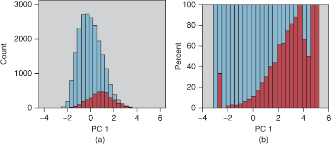
Figure 30.9 Component 1 values are highly predictive of response. (a) Histogram and (b) normalized histogram.
Here follow brief profiles of the remaining 10 components.
- Component 2: Promotion Proclivity. This component consists of five predictors, all except one related to past promotion activity: Promotion response rate, Promotions mailed, Total number of promotions on file, and Number of promotions responded to. The fifth predictor measures how long the customer has been on file. All predictors have positive weights, meaning they are all positively correlated.
- Component 3: Career Shopping. This component consists of three related types of clothing: Career pants, Jackets, and Collectibles (defined as mostly suits and career wear). These positively correlated predictors measure career clothing purchases.
- Component 4: Margin versus Markdown. This component consists of two negatively correlated predictors: Gross margin percentage and Markdown percentage. It makes sense that, as markdown increases, the margin will decrease. This component neatly captures this behavior.
- Component 5: Spending versus Returns. This component consists also consists of two negatively correlated variables: Average spending per visit and Percent returns. Evidently, those who have a high percentage of returns tend to have a low average spending amount per visit.
- Component 6: PS Store versus CC Store. Evidently these stores appeal to different groups of shoppers. If someone spends a lot at PS stores, they will tend not to spend much at CC stores, and vice versa.
- Component 7: Blouses versus Sweaters. It appears that shoppers tend not to buy blouses and sweaters together. The more spent on blouses, the less spent on sweaters, and vice versa.
- Component 8: Dresses. This is a singleton component containing only a single predictor: Dresses. In fact, each of the last four components is singleton. Note from Figure 30.3 that the eigenvalues for these components are each 1.2 or less, meaning that they explain about one predictor's worth of variability.
- Component 9: Suits. Singleton component: Suits. Perhaps surprising that it is not included in the Career Shopping component.
- Component 10: Shirts. Singleton component: Shirts.
- Component 11: Outerwear. Singleton component: Outerwear.
The question might arise: As the last four components are each singletons, why not just omit them, and extract only seven components? The answer is that the “singleton” label is a bit misleading. Each component contains loadings for each predictor; we have simply suppressed the small ones, in order to enhance interpretability. So, omitting these last four components would have effects beyond just these four predictors. Better to retain all 11 components.
30.5 Choosing the Optimal Number of Clusters Using Birch Clustering
Next, we turn to clustering. While PCA seeks to uncover groups of predictors with similar behavior, cluster analysis seeks to uncover groups of records with similar characteristics. One challenge for analysts performing cluster analysis is to select the optimal value of k, the number of clusters in the data. Here we illustrate two methods for selecting the optimal value of k, (i) using balanced iterative reducing and clustering using hierarchies (BIRCH) clustering on different sortings of the data and (ii) cycling through candidate values of k using k-means clustering.
In Chapter 21, we learned that one need not specify the optimal value of k when performing BIRCH clustering. The algorithm will itself choose the optimal value of k. Unfortunately, because it is tree-based, BIRCH clustering is sensitive to the order of the records scanned by the algorithm. In other words, it can report different clustering solutions for different sortings (orderings) of the data.
We shall then proceed as follows.
We select five as the number of different sortings of the training data set. The Modeler stream flow is shown in Figure 30.10. First, four new sort variables are derived, Sort2 – Sort5 (Sort1 is considered to be the original data ordering). Each of these derived variables assigns a random real number between 0.0 and 1.0 to each record. The records are then separately sorted by each sort variable. Then, BIRCH clustering is performed on each of the five data orderings, the original plus the four random sortings. Table 30.3 shows the value of k favored by BIRCH for each sorting. The clear winner for the optimal number of clusters using BIRCH clustering is k = 2.
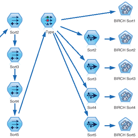
Figure 30.10 IBM/SPSS Modeler stream excerpt showing process for choosing k using BIRCH clustering.
Table 30.3 Value of k favored by BIRCH clustering for each sorting
| Sort1 | Sort2 | Sort3 | Sort4 | Sort5 |
| 2 | 2 | 2 | 2 | 2 |
30.6 Choosing the Optimal Number of Clusters Using k-Means Clustering
An alternate, and probably more widespread, method for selecting the optimal value for k is the following.
Here, we apply k-means clustering with k = 2, 3, and 4. The Modeler results are shown in Figure 30.11. The mean silhouette value for k = 2 is greater than that for the other values of k. Therefore, both methods concur that the optimal number of clusters in the data is k = 2.

Figure 30.11 Mean silhouette is greatest for k = 2.
30.7 Application of k-Means Clustering
We thus proceed to apply k-means clustering to the set of predictors in the training data set, including all the continuous variables from Figure 30.2, along with all the flag variables and nominal variables. The principal components are not included as inputs to the clustering algorithm. Of course, the response should not be included as input to any modeling algorithm. Graphical summaries of the resulting two clusters are provided in Figure 30.12. Not all predictors were helpful in discriminating between the clusters; these are omitted from Figure 30.12.

Figure 30.12 Graphical summaries of predictors, by cluster, for the training data.
30.8 Validating the Clusters
We use cross-validation to validate our clusters. We apply k-means clustering to the test data set, using the same set of predictors used for the training data set. The graphical summary results are shown in Figure 30.13. The results are broadly similar to what we uncovered using the training data set. There are two clusters, the larger of which represents a large set of casual shoppers, while the smaller cluster represents the faithful customers (see the cluster profiles below). There are some differences, such as ordering of the variables, but, on the whole, the clusters are validated.
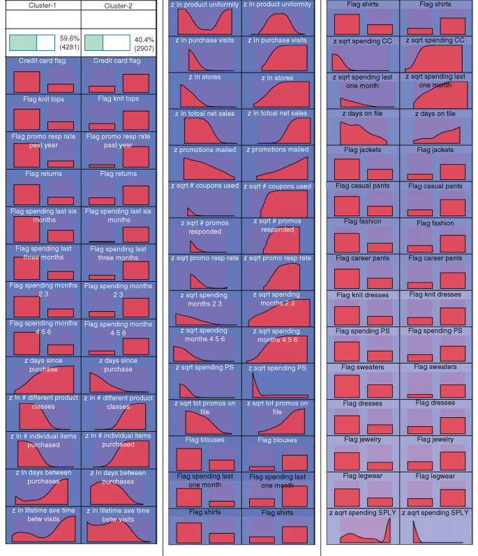
Figure 30.13 Graphical summaries of predictors, by cluster, for the test data set.
30.9 Profiling the Clusters
We can use the information in Figure 30.12 to construct descriptive profiles of the clusters, which are as follows.
- Cluster 1: Casual Shoppers Cluster 1 is the larger cluster, containing 58.6% of the customers. Cluster 1 contains lower proportions of positive values for all flag variables listed in Figure 30.12. This indicates for example that Cluster 1 contains lower incidence of credit card purchases, lower response to previous promotions, lower spending in previous time periods, and lower proportions of purchases in most clothing classes. Cluster 1 contains newer customers (days on file), who nevertheless wait longer between purchases. The casual shoppers tend to focus on a small number of product classes, and to purchase only a few different items. They have fewer than average purchase visits, visit fewer different stores, and have lower total net sales. Their promotion response rate is lower than average, as well as the number of coupons used.
- Cluster 2: Faithful Customers Cluster 2 is the smaller cluster, containing 41.4% of the customers, and represents the polar opposite of Cluster 1 in most respects. Cluster 2 contains higher proportions of positive values for all the listed flag variables. This indicates, for example, that Cluster 1 contains greater use of credit cards, higher response to previous promotions, higher spending in previous time periods, and higher proportions of purchases in most clothing classes. The faithful Cluster 2 customers have been shopping with us for a long time, while having smaller durations between purchases. Cluster 2 customers shop for a wide variety of goods, and purchase a higher than average number of different items. They have higher than average purchase visits, visit more stores, and have higher total net sales. Their promotion response rate is higher than average, as well as the number of coupons used.
Without question, these clusters reflect different real-world categories of shoppers, thereby underscoring their validity. One can imagine the store clerks learning some of the faithful customers' names by sight, while not recognizing many of the casual shoppers. We might anticipate that the faithful customers cluster will have a much stronger response to the direct-mail marketing promotion than the casual shoppers. In fact, this is the case, as is shown by the highlighted section of the contingency table of cluster membership versus response in Figure 30.14.
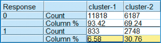
Figure 30.14 Faithful customers are more than four times as likely to respond to the direct-mail marketing promotion as casual shoppers.
To summarize, we have extracted principal components and clusters that have provided some insight into customer behaviors, as well as uncovered groups of predictors that behave similarly. These have helped us fulfill our secondary objective of developing better understanding of our clientele. In Chapter 31, we construct classification models that will help us to address our primary objective: maximizing profits.