
Chapter 14
NaïVe Bayes and Bayesian Networks
14.1 Bayesian Approach
In the field of statistics, there are two main approaches to probability. The usual way probability is taught, for example in most typical introductory statistics courses, represents the frequentist or classical approach. In the frequentist approach to probability, the population parameters are fixed constants whose values are unknown. These probabilities are defined to be the relative frequencies of the various categories, where the experiment is repeated an indefinitely large number of times. For example, if we toss a fair coin 10 times, it may not be very unusual to observe 80% heads; but if we toss the fair coin 10 trillion times, we can be fairly certain that the proportion of heads will be near 50%. It is this “long-run” behavior that defines probability for the frequentist approach.
However, there are situations for which the classical definition of probability is unclear. For example, what is the probability that terrorists will strike New York City with a dirty bomb? As such an occurrence has never occurred, it is difficult to conceive what the long-run behavior of this gruesome experiment might be. In the frequentist approach to probability, the parameters are fixed, and the randomness lies in the data, which are viewed as a random sample from a given distribution with unknown but fixed parameters.
The Bayesian approach to probability turns these assumptions around. In Bayesian statistics, the parameters are considered to be random variables, and the data are considered to be known. The parameters are regarded as coming from a distribution of possible values, and Bayesians look to the observed data to provide information on likely parameter values.
Let ![]() represent the parameters of the unknown distribution. Bayesian analysis requires elicitation of a prior distribution for
represent the parameters of the unknown distribution. Bayesian analysis requires elicitation of a prior distribution for ![]() , called the prior distribution,
, called the prior distribution, ![]() . This prior distribution can model extant expert knowledge, if any, regarding the distribution of
. This prior distribution can model extant expert knowledge, if any, regarding the distribution of ![]() . For example, churn1 modeling experts may be aware that a customer exceeding a certain threshold number of calls to customer service may indicate a likelihood to churn. This knowledge can be distilled into prior assumptions about the distribution of customer service calls, including its mean and standard deviation. If no expert knowledge regarding the prior distribution is available, Bayesian analysts may posit a so-called non-informative prior, which assigns equal probability to all values of the parameter. For example, the prior probability of both churners and non-churners could be set at 0.5, using a non-informative prior. (Note, if in this case, this assumption does not seem reasonable, then you must be applying your expert knowledge about churn modeling!) Regardless, because the field of data mining often encounters huge datasets, the prior distribution should be dominated by the overwhelming amount of information to be found in the observed data.
. For example, churn1 modeling experts may be aware that a customer exceeding a certain threshold number of calls to customer service may indicate a likelihood to churn. This knowledge can be distilled into prior assumptions about the distribution of customer service calls, including its mean and standard deviation. If no expert knowledge regarding the prior distribution is available, Bayesian analysts may posit a so-called non-informative prior, which assigns equal probability to all values of the parameter. For example, the prior probability of both churners and non-churners could be set at 0.5, using a non-informative prior. (Note, if in this case, this assumption does not seem reasonable, then you must be applying your expert knowledge about churn modeling!) Regardless, because the field of data mining often encounters huge datasets, the prior distribution should be dominated by the overwhelming amount of information to be found in the observed data.
Once the data have been observed, prior information about the distribution of ![]() can be updated, by factoring in the information about
can be updated, by factoring in the information about ![]() contained in the observed data. This modification leads to the posterior distribution,
contained in the observed data. This modification leads to the posterior distribution, ![]() , where X represents the entire array of data.
, where X represents the entire array of data.
This updating of our knowledge about ![]() from prior distribution to posterior distribution was first performed by the Reverend Thomas Bayes, in his Essay Towards Solving a Problem in the Doctrine of Chances,2 published posthumously in 1763.
from prior distribution to posterior distribution was first performed by the Reverend Thomas Bayes, in his Essay Towards Solving a Problem in the Doctrine of Chances,2 published posthumously in 1763.
The posterior distribution is found as follows: ![]() , where
, where ![]() represents the likelihood function,
represents the likelihood function, ![]() is the prior distribution, and
is the prior distribution, and ![]() is a normalizing factor called the marginal distribution of the data. As the posterior is a distribution rather than a single value, we can conceivably examine any possible statistic of this distribution that we are interested in, such as the first quartile, or the mean absolute deviation (Figure 14.1).
is a normalizing factor called the marginal distribution of the data. As the posterior is a distribution rather than a single value, we can conceivably examine any possible statistic of this distribution that we are interested in, such as the first quartile, or the mean absolute deviation (Figure 14.1).

Figure 14.1 The Reverend Thomas Bayes (1702–1761).
However, it is common to choose the posterior mode, the value of ![]() which maximizes
which maximizes ![]() , for an estimate, in which case we call this estimation method
, for an estimate, in which case we call this estimation method
the maximum a posteriori (MAP) method. For non-informative priors, the MAP estimate and the frequentist maximum-likelihood estimate often coincide, because the data dominate the prior. The likelihood function ![]() derives from the assumption that the observations are independently and identically distributed according to a particular distribution
derives from the assumption that the observations are independently and identically distributed according to a particular distribution ![]() , so that
, so that ![]() .
.
The normalizing factor ![]() is essentially a constant, for a given data set and model, so that we may express the posterior distribution such as this:
is essentially a constant, for a given data set and model, so that we may express the posterior distribution such as this: ![]() . That is, the posterior distribution of
. That is, the posterior distribution of ![]() , given the data, is proportional to the product of the likelihood and the prior. Thus, when we have a great deal of information coming from the likelihood, as we do in most data mining applications, the likelihood will overwhelm the prior.
, given the data, is proportional to the product of the likelihood and the prior. Thus, when we have a great deal of information coming from the likelihood, as we do in most data mining applications, the likelihood will overwhelm the prior.
Criticism of the Bayesian framework has mostly focused on two potential drawbacks. First, elicitation of a prior distribution may be subjective. That is, two different subject matter experts may provide two different prior distributions, which will presumably percolate through to result in two different posterior distributions. The solution to this problem is (i) to select non-informative priors if the choice of priors is controversial, and (ii) apply lots of data so that the relative importance of the prior is diminished. Failing this, model selection can be performed on the two different posterior distributions, using model adequacy and efficacy criteria, resulting in the choice of the better model. Is reporting more than one model a bad thing?
The second criticism has been that Bayesian computation has been intractable for most interesting problems, in data mining terms, where the approach suffered from scalability issues. The curse of dimensionality hits Bayesian analysis rather hard, because the normalizing factor requires integrating (or summing) over all possible values of the parameter vector, which may be computationally infeasible when applied directly. However, the introduction of Markov chain Monte Carlo (MCMC) methods such as Gibbs sampling and the Metropolis algorithm has greatly expanded the range of problems and dimensions that Bayesian analysis can handle.
14.2 Maximum A Posteriori (MAP) Classification
How do we find the MAP estimate of ![]() ? Well, we need the value of
? Well, we need the value of ![]() that will maximize
that will maximize ![]() ; this value is expressed as
; this value is expressed as ![]() , because it is the argument (value) that maximizes
, because it is the argument (value) that maximizes ![]() over all
over all ![]() . Then, using the formula for the posterior distribution, we have, because p(X) has no
. Then, using the formula for the posterior distribution, we have, because p(X) has no ![]() term:
term:
The Bayesian MAP classification is optimal; that is, it achieves the minimum error rate for all possible classifiers (Mitchell,3 page 174). Next, we apply these formulas to a subset of the churn data set,4 specifically, so that we may find the MAP estimate of churn for this subset.
First, however, let us step back for a moment and derive Bayes' theorem for simple events. Let A and B be events in a sample space. Then the conditional probability ![]() is defined as:
is defined as:
Also, ![]() . Now, re-expressing the intersection, we have
. Now, re-expressing the intersection, we have ![]() , and substituting, we obtain
, and substituting, we obtain
which is Bayes' theorem for simple events.
We shall restrict our example to only two categorical predictor variables, International Plan and Voice Mail Plan, and the categorical target variable, churn. The business problem is to classify new records as either churners or non-churners, based on the associations of churn with the two predictor variables learned in the training set. Now, how are we to think about this churn classification problem in the Bayesian terms addressed above? First, we let the parameter vector ![]() represent the dichotomous variable churn, taking on the two values true and false. For clarity, we denote
represent the dichotomous variable churn, taking on the two values true and false. For clarity, we denote ![]() as C for churn. The 3333 × 2 matrix X consists of the 3333 records in the data set, each with two fields, specifying either yes or no for the two predictor variables.
as C for churn. The 3333 × 2 matrix X consists of the 3333 records in the data set, each with two fields, specifying either yes or no for the two predictor variables.
Thus, equation (14.1) can be reexpressed as:
where I represents the International Plan and V represents the Voice Mail Plan. Denote:
- I to mean International Plan = yes
 to mean International Plan = no
- V to mean Voice Mail Plan = yes
 to mean Voice Mail Plan = no
- C to mean Churn = true
 to mean Churn = false.
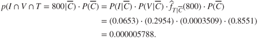
For example, for a new record containing ![]() , we seek to calculate the following probabilities, using equation (14.3):
, we seek to calculate the following probabilities, using equation (14.3):
For customers who churn (churners):
For customers who do not churn (non-churners):
We will then determine which value for churn produces the larger probability, and select it as ![]() , the MAP estimate of churn.
, the MAP estimate of churn.
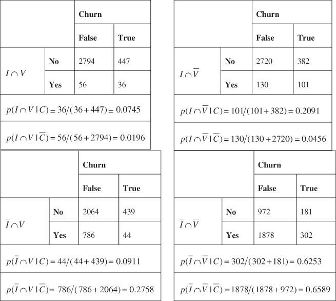
We begin by finding a series of marginal and conditional probabilities, all of which we shall use as we build toward our MAP estimates. Also, as we may examine the entire training data set of 3333 records, we may calculate the posterior probabilities directly, as given in Table 14.1.
Table 14.1 Posterior probabilities for the churn training data set
| Count | Count | Probability | |
| International Plan | No 3010 | Yes 323 | |
| Voice Mail Plan | No 2411 | Yes 922 | |
| Churn | False 2850 | True 483 | |
| International Plan, given churn = false | No 2664 | Yes 186 | |
| Voice Mail Plan, given churn = false | No 2008 | Yes 842 | |
| International Plan, given churn = true | No 346 | Yes 137 | |
| Voice Mail Plan, given churn = true | No 403 | Yes 80 |
Note that, using the probabilities given in Tables 14.2 and 14.1, we can easily find the complement of these probabilities by subtracting from 1. For completeness, we present these complement probabilities in Table 14.3.
Table 14.2 Marginal and conditional probabilities for the churn data set
| Count | Count | Probability | |
| Churn = true, given International Plan = yes | False 186 | True 137 | |
| Churn = true, given Voice Mail Plan = Yes | False 842 | True 80 |
Table 14.3 Complement probabilities for the churn training data set
| Complement Probabilities | |
Let us verify Bayes' theorem for this data set, using the probabilities in Table 14.2. ![]() , which is the value for this posterior probability given in Table 14.1.
, which is the value for this posterior probability given in Table 14.1.
We are still not in a position to calculate the MAP estimate of churn. We must first find joint conditional probabilities of the form ![]() . The contingency tables are shown in Table 14.4, allowing us to calculate joint conditional probabilities, by counting the records for which the respective joint conditions are held.
. The contingency tables are shown in Table 14.4, allowing us to calculate joint conditional probabilities, by counting the records for which the respective joint conditions are held.
Table 14.4 Joint conditional probabilities for the churn training data set
 |
Now we can find the MAP estimate of churn for the four combinations of International Plan and Voice Mail Plan membership, using equation (14.3):
Suppose we have a new record, where the customer belongs to the International Plan and Voice Mail Plan. Do we expect that this new customer will churn or not? That is, what will be the MAP estimate of churn for this new customer? We will apply equation (14.3) for each of the churn or non-churn cases, and select the classification that provides the larger value.
Here, we have:
For churners:
For non-churners:

As 0.0167 for churn = false is the maximum of the two cases, then ![]() , the MAP estimate of churn for this new customer, is churn = false. For customers belonging to both plans, this MAP estimate of “Churn = false” becomes our prediction; that is, we would predict that they would not churn.
, the MAP estimate of churn for this new customer, is churn = false. For customers belonging to both plans, this MAP estimate of “Churn = false” becomes our prediction; that is, we would predict that they would not churn.
Suppose a new customer belongs to the International Plan, but not the Voice Mail Plan. Then ![]() , and
, and
So that ![]() is churn = false.
is churn = false.
What if a new customer belongs to the Voice Mail Plan, but not the International Plan? Then ![]() , and
, and
Here again ![]() is churn = false.
is churn = false.
Finally, suppose a new customer belongs to neither the International Plan, nor the Voice Mail Plan. Then ![]() , and
, and
So that, yet again, ![]() is churn = false.
is churn = false.
14.3 Posterior Odds Ratio
Therefore, the MAP estimate for churn is false for each combination of International Plan and Voice Mail Plan membership. This result does not appear to be very helpful, because we will predict the same outcome for all customers regardless of their membership in the plans. However, not all of the classifications have the same strength of evidence. Next, we consider the level of evidence in each case, as defined by the posterior odds ratio. The posterior odds ratio represents a measure of the strength of evidence in favor of a particular classification, and is calculated as follows:
A posterior odds ratio of exactly 1.0 would mean that the evidence from the posterior distribution supports both classifications equally. That is, the combination of information from the data and the prior distributions does not favor one category over the other. A value greater than 1.0 indicates that the posterior distribution favors the positive classification, while a value less than 1.0 represents evidence against the positive classification (e.g., churn = true). The value of the posterior odds ratio may be interpreted as indicating roughly the proportion or ratio of evidence provided by the posterior distribution in favor of the positive classification against the negative classification.
In our example, the posterior odds ratio for a new customer who belongs to both plans is
This means that there is 64.67% as much evidence from the posterior distribution in support of churn = true as there is in support of churn = false for this customer.
For a new customer who belongs to the International Plan only, the posterior odds ratio is

indicating that there is 77.69% as much evidence from the posterior distribution in support of churn = true as there is in support of churn = false for such a customer.
New customers who belong to the Voice Mail Plan only have a posterior odds ratio of
indicating that there is only 5.6% as much evidence from the posterior distribution in support of churn = true as there is in support of churn = false for these customers.
Finally, for customers who belong to neither plan, the posterior odds ratio is

indicating that there is only 16.08% as much evidence from the posterior distribution in support of churn = true as there is in support of churn = false for customers who belong to neither plan.
Thus, although the MAP classification is churn = false in each case, the “confidence” in the classification varies greatly, with the evidence for churn = true ranging from 5.6% up to 77.69% of the evidence for churn = false. For the customers who belong to the International Plan, the evidence for churn is much stronger. In fact, note from the MAP calculations above that the joint conditional probabilities for customers belonging to the International Plan (with or without the Voice Mail Plan) favored churn = true, but were overwhelmed by the preponderance of non-churners in the data set, from 85.51% to 14.49%, so that the MAP classification turned out to be churn = false. Thus, the posterior odds ratio allows us to assess the strength of evidence for our MAP classifications, which is more helpful to the analyst than a simple up-or-down decision.
14.4 Balancing The Data
However, as the classification decision was influenced by the preponderance of non-churners in the data set, we may consider what might happen if we balanced the data set. Some data mining algorithms operate best when the relative frequencies of classes in the target variable are not extreme. For example, in fraud investigation, such a small percentage of transactions are fraudulent, that an algorithm could simply ignore such transactions, classify only non-fraudulent, and be correct 99.99% of the time. Therefore, balanced sampling methods are used to reduce the disparity among the proportions of target classes appearing in the training data.
In our case, we have 14.49% of the records representing churners, which may be considered somewhat uncommon, although one could argue otherwise. Nevertheless, let us balance the training data set, so that we have approximately 25% of the records representing churners. In Chapter 4, we learned two methods for balancing the data.
- Resample a number of rare records.
- Set aside a number of non-rare records.
Here we will balance the data by setting aside a number of the more common, non-churn records. This may be accomplished if we (i) accept all of the churn = true records, and (ii) take a random sample of 50% of our churn = false records. As the original data set had 483 churners and 2850 non-churners, this balancing procedure would provide us with ![]() churn = true records, as desired.
churn = true records, as desired.
Hence, using the balanced churn data set, we once again compute the MAP estimate for churn, for our four types of customers. Our updated probability of churning is
and for not churning is
For new customers who belong to the International Plan and Voice Mail Plan, we have
and
Thus, after balancing, ![]() , the MAP estimate of churn is churn = true, because 0.0189 is the greater value. Balancing has reversed the classification decision for this category of customers.
, the MAP estimate of churn is churn = true, because 0.0189 is the greater value. Balancing has reversed the classification decision for this category of customers.
For customers who belong to the International Plan only, we have
and
The MAP estimate ![]() is now churn = true, because 0.0529 is the greater value. Once again, balancing has reversed the original classification decision for this category of customers.
is now churn = true, because 0.0529 is the greater value. Once again, balancing has reversed the original classification decision for this category of customers.
For new customers belonging only to the Voice Mail Plan, we have
and
The MAP estimate has not changed from the original ![]() : churn = false for members of the Voice Mail Plan only.
: churn = false for members of the Voice Mail Plan only.
Finally, for new customers belonging to neither plan, we have
and
Again, the MAP estimate has not changed from the original ![]() : churn = false for customers belonging to neither plan.
: churn = false for customers belonging to neither plan.
In the original data, MAP estimates were churn = false for all customers, a finding of limited actionability. Balancing the data set has provided different MAP estimates for different categories of new customers, providing executives with simple and actionable results. We may of course proceed to compute the posterior odds ratio for each of these classification decisions, if we are interested in assessing the strength of evidence for the classifications. The reader is invited to do so in the exercises.
14.5 Naïve Bayes Classification
For our simplified example using two dichotomous predictors and one dichotomous target variable, finding the MAP classification posed no computational difficulties. However, Hand, Mannila, and Smyth5 (page 354) state that, in general, the number of probabilities that would need to be calculated to find the MAP classification would be on the order of ![]() , where k is the number of classes for the target variable, and m is the number of predictor variables. In our example, we had k = 2 classes in churn, and m = 2 predictors, meaning that we had to find four probabilities to render a classification decision, for example,
, where k is the number of classes for the target variable, and m is the number of predictor variables. In our example, we had k = 2 classes in churn, and m = 2 predictors, meaning that we had to find four probabilities to render a classification decision, for example, ![]() ,
, ![]() ,
, ![]() , and
, and ![]() .
.
However, suppose we are trying to predict the marital status (k = 5: single, married, divorced, widowed, separated) of individuals based on a set of m = 10 demographic predictors. Then, the number of probabilities to calculate would be on the order of ![]() probabilities. Note further that each of these 9,765,625 probabilities would need to be calculated based on relative frequencies of the appropriate cells in the 10-dimensional array. Using a minimum of 10 records per cell to estimate the relative frequencies, and on the unlikely assumption that the records are distributed uniformly across the array, the minimum requirement would be nearly 100 million records.
probabilities. Note further that each of these 9,765,625 probabilities would need to be calculated based on relative frequencies of the appropriate cells in the 10-dimensional array. Using a minimum of 10 records per cell to estimate the relative frequencies, and on the unlikely assumption that the records are distributed uniformly across the array, the minimum requirement would be nearly 100 million records.
Thus, MAP classification is impractical to apply directly to any interesting real-world data mining scenarios. What, then, can be done?
MAP classification requires that we find:
The problem is not calculating ![]() , for which there is usually a small number of classes. Rather, the problem is the curse of dimensionality; that is, finding
, for which there is usually a small number of classes. Rather, the problem is the curse of dimensionality; that is, finding ![]() for all the possible combinations of the X-variables (the predictors). Here is where the search space explodes, so, if there is a way to cut down on the search space for this problem, then it is to be found right here.
for all the possible combinations of the X-variables (the predictors). Here is where the search space explodes, so, if there is a way to cut down on the search space for this problem, then it is to be found right here.
Here is the key: Suppose we make the simplifying assumption that the predictor variables are conditionally independent, given the target value (e.g., churn = false). Two events A and B are said to be conditionally independent if, for a given event C, ![]() . For example, conditional independence would state that, for customers who churn, membership in one of the two plans (I or V) would not affect the probability of membership in the other plan. Similarly, the idea extends to customers who do not churn.
. For example, conditional independence would state that, for customers who churn, membership in one of the two plans (I or V) would not affect the probability of membership in the other plan. Similarly, the idea extends to customers who do not churn.
In general, the assumption of conditional independence may be expressed as follows:
The naïve Bayes classification is therefore ![]() .
.
When the conditional independence assumption is valid, the naïve Bayes classification is the same as the MAP classification. Therefore, we investigate whether the assumption of conditional independence holds for our churn data set example, as shown in Table 14.5. In each case, note that the approximation for the non-churners is several times closer than for the churners. This may indicate that the assumption of conditional independence assumption is best validated for non-rare categories, another argument in support of balancing when necessary.
Table 14.5 Checking the conditional independence assumption for churn data set
 |
We now proceed to calculate naïve Bayes classifications for the churn data set. For a new customer belonging to both plans, we have for churners,
and for non-churners,
The naïve Bayes classification for new customers who belong to both plans is therefore churn = false because 0.0165 is the larger of the two values. It turns out that, just as for the MAP classifier, all four cases return a naïve Bayes classification of churn = false. Also, after ![]() balancing, new customers who belong to the International Plan are classified by naïve Bayes as churners, regardless of Voice Mail Plan membership, just as for the MAP classifier. These results are left to the exercises for verification.
balancing, new customers who belong to the International Plan are classified by naïve Bayes as churners, regardless of Voice Mail Plan membership, just as for the MAP classifier. These results are left to the exercises for verification.
When using naïve Bayes classification, far fewer probabilities need to be estimated, just ![]() probabilities rather than
probabilities rather than ![]() for the MAP classifier; in other words, just the number of predictor variables times the number of distinct values of the target variable. In the marital status example, where we had k = 5 distinct marital statuses and m = 10 predictor variables, we would need to compute only
for the MAP classifier; in other words, just the number of predictor variables times the number of distinct values of the target variable. In the marital status example, where we had k = 5 distinct marital statuses and m = 10 predictor variables, we would need to compute only ![]() probabilities, rather than the 9.7 million needed for the MAP classifier. At 10 records per cell, that would mean that only 500 records would be needed, compared to the nearly 100 million calculated earlier. Clearly, the conditional independence assumption, when valid, makes our computational life much easier. Further, as the naïve Bayes classification is the same as the MAP classification when the conditional independence assumption is met, then the naïve Bayes classification is also optimal, in the sense of minimizing the error rate over all classifiers. In practice, however, departures from the conditional independence assumption tend to inhibit the optimality of the naïve Bayes classifier.
probabilities, rather than the 9.7 million needed for the MAP classifier. At 10 records per cell, that would mean that only 500 records would be needed, compared to the nearly 100 million calculated earlier. Clearly, the conditional independence assumption, when valid, makes our computational life much easier. Further, as the naïve Bayes classification is the same as the MAP classification when the conditional independence assumption is met, then the naïve Bayes classification is also optimal, in the sense of minimizing the error rate over all classifiers. In practice, however, departures from the conditional independence assumption tend to inhibit the optimality of the naïve Bayes classifier.
The conditional independence assumption should not be made blindly. Correlated predictors, for example, violate the assumption. For example, in classifying risk for credit default, total assets and annual income would probably be correlated. However, naïve Bayes would, for each classification (default, no default), consider total assets and annual income to be independent and uncorrelated. Of course, careful data mining practice includes dealing with correlated variables at the exploratory data analysis (EDA) stage anyway, because the correlation can cause problems for several different data methods. Principal components analysis can be used to handle correlated variables. Another option is to construct a user-defined composite, a linear combination of a small set of highly correlated variables. (See Chapter 1 for more information on handling correlated variables.)
14.6 Interpreting The Log Posterior Odds Ratio
Next, we examine the log of the posterior odds ratio, which can provide us with an intuitive measure of the amount that each variable contributes toward the classification decision. The posterior odds ratio takes the form:

which is the form of the posterior odds ratio for naïve Bayes.
Next, consider the log of the posterior odds ratio. As the log of a product is the sum of the logs, we have:

This form of the log posterior odds ratio is useful from an interpretive point of view, because each term,
relates to the additive contribution, either positive or negative, of each attribute.
For example, consider the log posterior odds ratio for a new customer who belongs to both the International Plan and Voice Mail Plan. Then, for the International Plan, we have

and for the Voice Mail Plan, we have
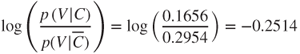
Thus, we see that membership in the International Plan contributes in a positive way to the likelihood that a particular customer will churn, while membership in the Voice Mail Plan decreases the churn probability. These findings concur with our exploratory results from Chapter 3, Exploratory Data Analysis.
14.7 Zero-Cell Problem
As we saw in Chapter 13, Logistic Regression, a cell with frequency zero can pose difficulties for the analysis. Now, for naïve Bayes estimation, what if a particular cell (combination of attribution values) has a zero frequency? For example, of the 483 customers who churned, 80 had the Voice Mail Plan, so that ![]() . However, suppose none of the churners had the Voice Mail Plan. Then
. However, suppose none of the churners had the Voice Mail Plan. Then ![]() would equal
would equal ![]() . The real problem with this is that, because the conditional independence assumption means that we take the product of the marginal probabilities, this zero value for
. The real problem with this is that, because the conditional independence assumption means that we take the product of the marginal probabilities, this zero value for ![]() will percolate through and dominate the result. As the naïve Bayes classification contains
will percolate through and dominate the result. As the naïve Bayes classification contains ![]() , a single zero probability in this product will render the entire product to be zero, which will also make
, a single zero probability in this product will render the entire product to be zero, which will also make ![]() equal to zero, thereby effectively eliminating this class (churn = true) from consideration for any future probability involving the Voice Mail Plan.
equal to zero, thereby effectively eliminating this class (churn = true) from consideration for any future probability involving the Voice Mail Plan.
To avoid this problem, we posit an additional number of “virtual” samples, which provides the following adjusted probability estimate for zero-frequency cells:
The constant ![]() represents the additional number of virtual samples used to find the adjusted probability, and controls how heavily the adjustment is weighted. The prior probability estimate p may be assigned, in the absence of other information, to be the non-informative uniform prior
represents the additional number of virtual samples used to find the adjusted probability, and controls how heavily the adjustment is weighted. The prior probability estimate p may be assigned, in the absence of other information, to be the non-informative uniform prior ![]() , where k is the number of classes for the target variable. Thus,
, where k is the number of classes for the target variable. Thus, ![]() additional samples, distributed according to p, are contributed to the calculation of the probability.
additional samples, distributed according to p, are contributed to the calculation of the probability.
In our example, we have n = 483, ![]() , and
, and ![]() . We choose
. We choose ![]() to minimize the effect of the intervention. The adjusted probability estimate for the zero probability cell for
to minimize the effect of the intervention. The adjusted probability estimate for the zero probability cell for ![]() is therefore:
is therefore: ![]() .
.
14.8 Numeric Predictors for Naïve Bayes Classification
Bayesian classification can be extended from categorical to continuous predictor variables, provided we know the relevant probability distribution. Suppose that, in addition to International Plan and Voice Mail Plan, we also had access to Total Minutes, the total number of minutes used by the cell-phone customer, along with evidence that the distribution of Total Minutes is normal, for both churners and non-churners. The mean Total Minutes for churners is ![]() minutes, with a standard deviation of
minutes, with a standard deviation of ![]() minutes. The mean Total Minutes for non-churners is
minutes. The mean Total Minutes for non-churners is ![]() with a standard deviation of
with a standard deviation of ![]() minutes. Thus, we assume that the distribution of Total Minutes for churners is
minutes. Thus, we assume that the distribution of Total Minutes for churners is ![]() and for non-churners is
and for non-churners is ![]() .
.
Let Tchurn represent the random variable Total Minutes for churners. Then,

with an analogous form for non-churners. (Here, ![]() represents
represents ![]() .)
.)
Also, ![]() is substituted for
is substituted for ![]() , because, for continuous random variables,
, because, for continuous random variables, ![]() .
.
Next, suppose we are interested in classifying new customers who have 800 Total Minutes, and belong to both plans, using naïve Bayes classification. We have:
For churners:

and for non-churners:

Hence, the naïve Bayes classification for new customers who have 800 Total Minutes and belong to both plans is churn = true, by a posterior odds ratio of
In other words, the additional information that the new customer had 800 Total Minutes was enough to reverse the classification from churn = false (previously, without Total Minutes) to churn = true. This is due to the somewhat heavier cell-phone usage of the churners group, with a higher mean Total Minutes.
Now, assumptions of normality should not be made without supporting evidence. Consider Figure 14.2, a comparison dot plot of the two distributions. Immediately we can see that indeed there are many more non-churner records than churners. We also note that the balancing point (the mean, indicated by the triangle) for churners is greater than for non-churners, supporting the above statistics. Finally, we notice that the normality assumption for non-churners looks quite solid, while the normality assumption for the churners looks a little shaky.
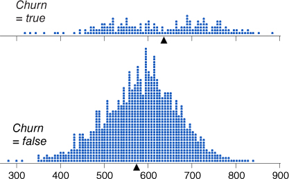
Figure 14.2 Comparison dot plot of Total Minutes for churners and non-churners.
Normal probability plots are then constructed for the two distributions just described, and shown in Figure 14.3. In a normal probability plot, there should be no systematic deviations from linearity; otherwise, the normality assumption is called into question. In Figure 14.3, the bulk of the points for the non-churners line up nearly perfectly on a straight line, indicating that the normality assumption is validated for non-churners' Total Minutes. However, there does appear to be systematic curvature in the churners' data points, in a slight backwards S-curve, indicating that the normality assumption for churners' Total Minutes is not validated. As the assumption is not validated, then all subsequent inference applying this assumption must be flagged as such for the end-user. For example, the naïve Bayes classification of churn = true may or may not be valid, and the end-user should be informed of this uncertainty.
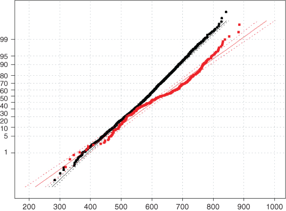
Figure 14.3 Normal probability plots of Total Minutes for churners and non-churners.
Often, non-normal distribution can be transformed to normality, using, for example, the Box–Cox transformation ![]() . However, Figure 14.2 shows that Total Minutes for churners actually looks like a mixture of two normal distributions, which will prove resistant to monotonic transformations to normality. The mixture idea is intriguing and deserves further investigation, which we do not have space for here. Data transformations were investigated more fully in Chapters 8 and 9.
. However, Figure 14.2 shows that Total Minutes for churners actually looks like a mixture of two normal distributions, which will prove resistant to monotonic transformations to normality. The mixture idea is intriguing and deserves further investigation, which we do not have space for here. Data transformations were investigated more fully in Chapters 8 and 9.
Alternatively, one may dispense with the normality assumption altogether, and choose to work directly with the observed empirical distribution of Total Minutes for churners and non-churners. We are interested in comparing the ![]() for each distribution; why not estimate this probability by directly estimating
for each distribution; why not estimate this probability by directly estimating ![]() for each distribution? It turns out that three of the churner customers had between 798 and 802 total minutes, compared to one for the non-churner customers. So, the probability estimates would be
for each distribution? It turns out that three of the churner customers had between 798 and 802 total minutes, compared to one for the non-churner customers. So, the probability estimates would be ![]() for the churners, and
for the churners, and ![]() for the non-churners.
for the non-churners.
Thus, to find the naïve Bayes classification for churners,

and for non-churners,
(Here, ![]() represents our empirical estimate of
represents our empirical estimate of ![]() .)
.)
Thus, once again, the naïve Bayes classification for new customers who have 800 Total Minutes and belong to both plans is churn = true, this time by a posterior odds ratio of ![]() . The evidence is even more solid in favor of a classification of churn = true for these customers, and we did not have to burden ourselves with an assumption about normality.
. The evidence is even more solid in favor of a classification of churn = true for these customers, and we did not have to burden ourselves with an assumption about normality.
The empirical probability estimation method shown here should be verified over a range of margins of error. Above, we found the numbers of records within a margin of error of 2 records ![]() . The reader may verify that that there are 8 churn records and 3 non-churn records within 5 minutes of the desired 800 minutes; and that there are 15 churn records and 5 non-churn records within 10 minutes of the desired 800 minutes. So the approximate 3 : 1 ratio of churn records to non-churn records in this area of the distribution seems fairly stable.
. The reader may verify that that there are 8 churn records and 3 non-churn records within 5 minutes of the desired 800 minutes; and that there are 15 churn records and 5 non-churn records within 10 minutes of the desired 800 minutes. So the approximate 3 : 1 ratio of churn records to non-churn records in this area of the distribution seems fairly stable.
14.9 WEKA: Hands-on Analysis Using Naïve Bayes
In this exercise, Waikato Environment for Knowledge Analysis's (WEKA's) naïve Bayes classifier is used to classify a small set of movie reviews as either positive (pos) or negative (neg). First, the text from 20 actual reviews is preprocessed to create a training file movies_train.arff containing three Boolean attributes and a target variable. This file is used to train our naïve Bayes model and contains a set of 20 individual review instances, where 10 reviews have the class value “pos,” and the remaining 10 reviews take on the class value “neg.” Similarly, a second file is created to test our model. In this case, movies_test.arff only contains four review instances, where two are positive and the remaining two are negative.
During the preprocessing stage, the unigrams (specifically adjectives) are extracted from the reviews and a list of adjectives is derived. The three most frequently occurring adjectives are chosen from the list and form the set of attributes used by each review instance. Specifically, each instance is represented as a Boolean document vector of length three, where each attribute's value is either 1 or 0, corresponding to whether the review contains or does not contain the particular adjective, respectively. The Attribute-Relation File Format (ARFF)-based training file movies_train.arff is shown in Table 14.6.
Table 14.6 ARFF Movies Training Filemovies_train.arff.
 |
All attributes in the ARFF file are nominal and take on one of two values; inputs are either “0” or “1,” and the target variable CLASS is either “pos” or “neg.” The data section lists each instance, which corresponds to a specific movie review record. For example, the third line in the data section corresponds to a review where more = 1, much = 1, other = 0, and CLASS = neg.
Now, we load the training file and build the naïve Bayes classification model.
- Click Explorer from the WEKA GUI Chooser dialog.
- On the Preprocess tab, press Open file and specify the path to the training file, movies_train.arff.
- Select the Classify tab.
- Under Classifier, press the Choose button
- Select Classifiers → Bayes → Naïve Bayes from the navigation hierarchy.
- In our modeling experiment, we have separate training and test sets; therefore, under Test options, choose the Use training set option.
- Click Start to build the model.
WEKA creates the naïve Bayes model and produces the results in the Classifier output window as shown in Figure 14.4. In general, the results indicate that the classification accuracy of the model, as measured against the training set, is ![]() .
.
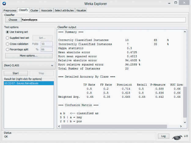
Figure 14.4 WEKA Explorer: naïve Bayes training results.
Next, our model is evaluated against the unseen data found in the test set, movies_test.arff.
- Under Test options, choose Supplied test set. Click Set.
- Click Open file, specify the path to the test file, movies_test.arff. Close the Test Instances dialog.
- Check the Output text predictions on test set option. Click OK.
Click the Start button to evaluate the model against the test set.
Surprisingly, the Explorer Panel shows that our naïve Bayes model has classified all four movie reviews in the test set correctly. Although these results are encouraging, from a real-world perspective, the training set lacks a sufficient number of both attributes and examples to be considered practical in any real sense. We continue with the objective of becoming familiar with the naïve Bayes classifier. Let us explore how naïve Bayes arrived at the decision to classify the fourth record in the test set correctly. First, however, we examine the probabilities reported by the naïve Bayes classifier.
The naïve Bayes model reports the actual probabilities it used to classify each review instance from the test set as either “pos” or “neg.” For example, Table 14.7 shows that naïve Bayes has classified the fourth instance from the test set as “pos” with a probability equal to 0.60.
Table 14.7 Naive bayes test set predictions
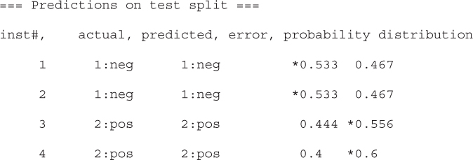 |
In Table 14.8, the conditional probabilities are calculated that correspond to the data found in movies_train.arff. For example, given that the review is negative, the conditional probability of the word “more” occurring is ![]() . In addition, we also know the prior probabilities of
. In addition, we also know the prior probabilities of ![]() . These simply correspond with the fact that our training set is balanced
. These simply correspond with the fact that our training set is balanced ![]() .
.
Table 14.8 Conditional probabilities derived from movies_training.arff
| more | much | other | |||
| neg | |||||
| 1 | 0 | 1 | 0 | 1 | 0 |
| 9/10 | 1/10 | 7/10 | 3/10 | 5/10 | 5/10 |
| pos | |||||
| 1 | 0 | 1 | 0 | 1 | 0 |
| 8/10 | 2/10 | 6/10 | 4/10 | 7/10 | 3/10 |
Recall the method of adjusting the probability estimate to avoid zero-frequency cells, as described earlier in the chapter. In this particular case, naïve Bayes produces an internal adjustment, where ![]() and
and ![]() , to produce
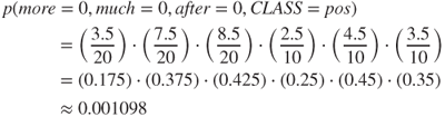
, to produce ![]() . Therefore, we now calculate the probably of the fourth review from the test as set being either “pos” or “neg”:
. Therefore, we now calculate the probably of the fourth review from the test as set being either “pos” or “neg”:
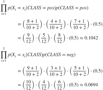
Finally, we normalize the probabilities and determine:
Here, the review is classified as positive with a 0.60 probability. These results agree with those reported by WEKA in Table 14.7, which also classified the review as positive. In fact, our hand-calculated probabilities match those reported by WEKA. Although the data set used for this example is rather small, it demonstrates the use of the naïve Bayes classifier in WEKA when using separate training and test files. More importantly, our general understanding of the algorithm has increased, as a result of computing the probabilities that led to an actual classification by the model.
14.10 Bayesian Belief Networks
Naïve Bayes classification assumes that the attributes are conditionally independent, given the value of the target variable. This assumption may in fact be too strong for environments where dependence exists among the predictor variables. Bayesian belief networks (BBNs) are designed to allow joint conditional independencies to be defined among subsets of variables. BBNs, also called Bayesian networks or Bayes nets, take the form of a directed acyclic graph (DAG), where directed means that the arcs are traversed in one direction only, and acyclic means that no child node cycles backup to any progenitor.
An example of a Bayesian network in the form of a DAG is shown in Figure 14.5. The nodes represent variables, and the arcs represent the (directed) dependence among the variables. In general, Node A is a parent or immediate predecessor of Node X, and Node X is a descendant of Node A, if there exists a directed arc from A to X. The intrinsic relationship among the variables in a Bayesian network is as follows:
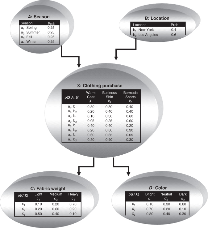
Figure 14.5 A Bayesian network for the clothing purchase example.
Each variable in a Bayesian network is conditionally independent of its non-descendants in the network, given its parents.
Thus, we have:
Note that the child node probability depends only on its parents.
14.11 Clothing Purchase Example
To introduce Bayesian networks, we shall use the clothing purchase example, illustrated by the Bayes net in Figure 14.5. Suppose a clothes retailer operates two outlets, one in New York and one in Los Angeles, each producing sales throughout the four seasons. The retailer is interested in probabilities concerning three articles of clothing, in particular, warm coats, business shirts, and Bermuda shorts. Questions of interest include the fabric weight of the article of clothing (light, medium, or heavy), and the color of the article (bright, neutral, or dark).
To build a Bayesian network, there are two main considerations:
- What is the dependence relationship among the variables of interest?
- What are the associated “local” probabilities?
The retailer has five variables: season, location, clothing purchase, fabric weight, and color. What is the dependence relationship among these variables? For example, does the season of the year depend on the color of the clothes purchased? Certainly not, because a customer's purchase of some bright clothing does not mean that spring is here, for example, although the customer may wish it so. In fact, the season of the year does not depend on any of the other variables, and so we place the node for the variable season at the top of the Bayes network, which indicates that it does not depend on the other variables. Similarly, location does not depend on the other variables, and is therefore placed at the top of the network.
As the fabric weight and the color of the clothing is not known until the article is purchased, the node for the variable clothing purchase is inserted next into the network, with arcs to each of the fabric weight and color nodes.
The second consideration for constructing a Bayesian network is to specify all of the entries in the probability tables for each node. The probabilities in the season node table indicate that clothing sales for this retail establishment are uniform throughout the four seasons. The probabilities in the location node probability table show that 60% of sales are generated from their Los Angeles store, and 40% from their New York store. Note that these two tables need not supply conditional probabilities, because the nodes are at the top of the network.
Assigning probabilities for clothing purchase requires that the dependence on the parent nodes be taken into account. Expert knowledge or relative frequencies (not shown) should be consulted. Note that the probabilities in each row of the table sum to one. For example, the fourth row of the clothing purchase table shows the conditional probabilities of purchasing the articles of clothing from the Los Angeles store in the summer. The probabilities of purchasing a warm coat, a business shirt, and Bermuda shorts are 0.05, 0.35, and 0.60, respectively. The seventh row represents probabilities of purchasing articles of clothing from the New York store in winter. The probabilities of purchasing a warm coat, a business shirt, and Bermuda shorts are 0.60, 0.35, 0.05, respectively.
Given a particular item of clothing, the probabilities then need to be specified for fabric weight and color. A warm coat will have probabilities for being of light, medium, or heavy fabric or 0.10, 0.20, and 0.70, respectively. A business shirt will have probabilities of having bright, neutral, or dark color of 0.70, 0.20, and 0.10, respectively. Note that the fabric weight or color depends only on the item of clothing purchased, and not the location or season. In other words, color is conditionally independent of location, given the article of clothing purchased. This is one of the relationships of conditional independence to be found in this Bayesian network. Given below is some of the other relationships:
- Color is conditionally independent of season, given clothing purchased.
- Color is conditionally independent of fabric weight, given clothing purchased.
- Fabric weight is conditionally independent of color, given clothing purchased.
- Fabric weight is conditionally independent of location, given clothing purchased.
- Fabric weight is conditionally independent of season, given clothing purchased.
Note that we could say that season is conditionally independent of location, given its parents. But as season has no parents in the Bayes net, this means that season and location are (unconditionally) independent.
Be careful when inserting arcs into the Bayesian network, because these represent strong assertions of conditional independence.
14.12 Using The Bayesian Network to Find Probabilities
Next, suppose we would like to find the probability that a given purchase involved light-fabric, neutral-colored Bermuda shorts were purchased in New York in the winter. Using equation (14.4), we may express what we seek as:

Evidently, there is not much demand for light-fabric, neutral-colored Bermuda shorts in New York in the winter.
Similarly, probabilities may be found in this way for any combinations of season, location, article of clothing, fabric weight, and color. Using the Bayesian network structure, we can also calculate prior probabilities for each node. For example, the prior probability of a warm coat is found as follows:

So the prior probability of purchasing a warm coat is 0.2525. Note that we used the information that season and location are independent, so that ![]() . For example, the probability that a sale is made in the spring in New York is
. For example, the probability that a sale is made in the spring in New York is ![]() .
.
Posterior probabilities may also be found. For example,
To find ![]() , we must first find
, we must first find ![]() and
and ![]() . Using the conditional probability structure of the Bayesian network in Figure 14.5, we have
. Using the conditional probability structure of the Bayesian network in Figure 14.5, we have

So, ![]() .
.
Thus, we have ![]() . Then the Bayes net could provide a classification decision using the highest posterior probability, among
. Then the Bayes net could provide a classification decision using the highest posterior probability, among ![]() ,
, ![]() ,
, ![]() , and
, and ![]() (see Exercises).
(see Exercises).
A Bayesian network represents the joint probability distribution for a given set of variables. What is a joint probability distribution? Let ![]() represent a set of m random variables, with each random variable
represent a set of m random variables, with each random variable ![]() defined on space
defined on space ![]() . For example, a normal random variable X is defined on space
. For example, a normal random variable X is defined on space ![]() , where
, where ![]() is the real number line. Then the joint space of
is the real number line. Then the joint space of ![]() is defined as the Cartesian product
is defined as the Cartesian product ![]() . That is, each joint observation consists of the vector of length m of observed field values
. That is, each joint observation consists of the vector of length m of observed field values ![]() . The distribution of these observations over the joint space is called the joint probability distribution.
. The distribution of these observations over the joint space is called the joint probability distribution.
The Bayesian network represents the joint probability distribution by providing (i) a specified set of assumptions regarding the conditional independence of the variables, and (ii) the probability tables for each variable, given its direct predecessors. For each variable, information regarding both (i) and (ii) are provided.
For a subset of variables, ![]() , the joint probability may be found thus:
, the joint probability may be found thus:
where we define ![]() to be the set of immediate predecessors of
to be the set of immediate predecessors of ![]() in the network. The probabilities
in the network. The probabilities ![]() are the probabilities that have been specified in the probability table associated with the node for
are the probabilities that have been specified in the probability table associated with the node for ![]() .
.
How does learning take place in a Bayesian network? When the structure of the network is known, and the field values have all been observed, then learning in Bayesian nets is straightforward. The local (node-specific) probability tables are fully specified, and any desired joint, conditional, prior, or posterior probability may be calculated.
However, when some of the field values are hidden or unknown, then we need to turn to other methods, with the goal of filling in all the entries in the local probability distribution table. Russell et al.6 suggest a gradient descent method for learning in Bayesian networks. In this paradigm, the unknown entries in the probability distribution tables are considered to be unknown weights, and gradient descent methods, analogous to the neural network learning case (Chapter 12 of this book, or Chapter 4 of Mitchell7), can be applied to find the optimal set of weights (probability values), given the data.
Bayes nets were originally designed to aid subject matter experts to graphically specify the conditional independence structure among variables. However, analysts may also attempt to discern the unknown structure of Bayes nets by studying the dependence and independence relationships among the observed variable values. Sprites, Glymour, and Scheines8 and Ramoni and Sebastian9 provide further information about learning both the content and structure of Bayesian networks.
14.12.1 WEKA: Hands-On Analysis Using Bayes Net
Let us revisit the movies data set; however, this time, classification of the data is explored using WEKA's Bayes net classifier. Similarly to our last experiment, the 20 instances in movies_train.arff are used to train our model, whereas it is tested using the four reviews in movies_test.arff. Let us begin by loading the training file.
- Click Explorer from the WEKA GUI Chooser dialog.
- On the Preprocess tab, press Open file and specify the path to the training file, movies_train.arff.
- If successful, the Explorer Panel looks similar to Figure 14.6, and indicates the relation movies_train.arff consists of 20 instances with four attributes. It also shows, by default, that CLASS is specified as the class variable for the data set. Next, select the Classify tab.
- Under Classifier, press the Choose button.
- Select Classifiers → Bayes → BayesNet from the navigation hierarchy.
- Under Test options, specify Supplied training set.
- Click Start.
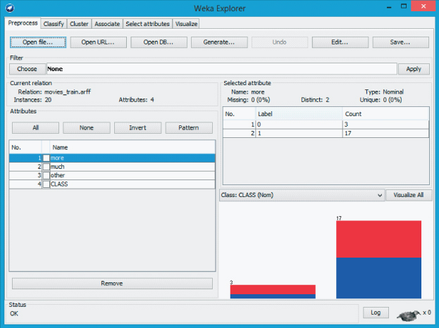
Figure 14.6 WEKA explorer panel: preprocess tab.
The results are reported in the Classifier output window. The classification accuracy for Bayes net is 65% (13/20), which is identical to the results reported by naïve Bayes. Again, let us evaluate our classification model using the data from movies_test.arff, with the goal of determining the probabilities by which Bayes net classifies these instances.
- Under Test options, choose Supplied test set. Click Set.
- Click Open file, specify the path to the test file, movies_test.arff. Close the Test Instances dialog.
- Next, click the More options button.
- Check the Output text predictions on test set option. Click OK.
- Click the Start button to evaluate the model against the test set.
Now, the predictions for each instance, including their associated probability, are reported in the Classifier output window. For example, Bayes net correctly classified instance three as “pos,” with probability 0.577, as shown in Table 14.9. Next, let us evaluate how Bayes net made its classification decision for the third instance.
Table 14.9 Bayes net test set predictions
 |
First, recall the data set used to build our model, as shown in Table 14.6. From here the prior probabilities for the attributes more, much, and other can be derived; for example, ![]() and
and ![]() . In addition, to avoid zero-probability cells, Bayes net uses a simple estimation method that adds 0.5 to each cell count. Using this information, the prior probability tables for the three parent nodes used in the network are shown in Table 14.10.
. In addition, to avoid zero-probability cells, Bayes net uses a simple estimation method that adds 0.5 to each cell count. Using this information, the prior probability tables for the three parent nodes used in the network are shown in Table 14.10.
Table 14.10 Prior probabilities derived from movies_training.arff.
| more | much | other | |||
| 1 | 0 | 1 | 0 | 1 | 0 |
| 17.5/20 | 3.5/20 | 13.5/20 | 7.5/20 | 12.5/20 | 8.5/20 |
Now, according to the model built from the training set data, we calculate the probability of classifying the third record from the test set as “pos” using the formula:

As described above, Bayes net also adds 0.5 to the conditional probability table cell counts to prevent zero-based probabilities from occurring. For example, the conditional probability ![]() becomes
becomes ![]() using this internal adjustment. Therefore, the probability of a positive classification, given the values for more, much, and other found in the third instance, is computed as follows:
using this internal adjustment. Therefore, the probability of a positive classification, given the values for more, much, and other found in the third instance, is computed as follows:
Likewise, the probability of a negative classification is derived using a similar approach:

Our last step is to normalize the probabilities as follows:

Our calculations have determined that, according to the Bayes net model built from the training set, instance three is classified as positive with probability 0.577. Again, our hand-calculated probabilities agree with those produced by the WEKA model, as shown in Table 14.9. Clearly, our results indicate that “hand-computing” the probability values for a network of moderate size is a nontrivial task.
R References
- R Core Team. R: A Language and Environment for Statistical Computing. Vienna, Austria: R Foundation for Statistical Computing; 2012. 3-900051-07-0, http://www.R-project.org/. Accessed 2014 Oct 07.
Exercises
Clarifying the Concepts
1. Describe the differences between the frequentist and Bayesian approaches to probability.
2. Explain the difference between the prior and posterior distributions.
3. Why would we expect, in most data mining applications, the maximum a posteriori estimate to be close to the maximum-likelihood estimate?
4. Explain in plain English what is meant by the maximum a posteriori classification.
5. Explain the interpretation of the posterior odds ratio. Also, why do we need it?
6. Describe what balancing is, and when and why it may be needed. Also, describe two techniques for achieving a balanced data set, and explain why one method is preferred.
7. Explain why we cannot avoid altering, even slightly, the character of the data set, when we apply balancing.
8. Explain why the MAP classification is impractical to apply directly for any interesting real-world data mining application.
9. What is meant by conditional independence? Provide an example of events that are conditionally independent. Now provide an example of events that are not conditionally independent.
10. When is the naïve Bayes classification the same as the MAP classification? What does this mean for the naïve Bayes classifier, in terms of optimality?
11. Explain why the log posterior odds ratio is useful. Provide an example.
12. Describe the process for using continuous predictors in Bayesian classification, using the concept of distribution.
13. Extra credit: Investigate the mixture idea for the continuous predictor mentioned in the text.
14. Explain what is meant by working with the empirical distribution. Describe how this can be used to estimate the true probabilities.
15. Explain the difference in assumptions between naïve Bayes classification and Bayesian networks.
16. Describe the intrinsic relationship among the variables in a Bayesian network.
17. What are the two main considerations when building a Bayesian network?
Working With The Data
18. Compute the posterior odds ratio for each of the combinations of International Plan and Voice Mail Plan membership, using the balanced data set.
19. Calculate the naïve Bayes classification for all four possible combinations of International Plan and Voice Mail Plan membership, using the ![]() balancing.
balancing.
20. Verify the empirical distribution results referred to in the text, of the numbers of records within the certain margins of error of 800 minutes, for each of churners and non-churners.
21. Find the naïve Bayes classifier for the following customers. Use the empirical distribution where necessary.
- Belongs to neither plan, with 400 day minutes.
- Belongs to the International Plan only, with 400 minutes.
- Belongs to both plans, with 400 minutes.
- Belongs to both plans, with zero minutes. Comment.
22. Provide the MAP classification for season given that a warm coat was purchased, in the clothing purchase example in the Bayesian network section.
23. Revisit the WEKA naïve Bayes example. Calculate the probability that the first instance in movies_test.arff is “pos” and “neg.” Do your calculations agree with those reported by WEKA leading to a negative classification?
24. Compute the probabilities by which the Bayes net model classifies the fourth instance from the test file movies_test.arff. Do your calculations result in a positive classification as reported by WEKA?
Hands-On Analysis
For Exercises 25–35, use the breast cancer data set. This data set was collected by Dr. William H. Wohlberg from the University of Wisconsin Hospitals, Madison. Ten numeric predictors are used to predict the class of malignant breast cancer tumor (class = 1), as opposed to a benign tumor (class = 0).
25. Consider using only two predictors, mitoses and clump thickness, to predict tumor class. Categorize the values for mitoses as follows: Low = 1 and High = 2–10. Categorize the values for clump thickness as follows: Low = 1–5 and High = 6–10. Discard the original variables and use these categorized predictors.
26. Find the prior probabilities for each of the predictors and the target variable. Find the complement probabilities of each.
27. Find the conditional probabilities for each of the predictors, given that the tumor is malignant. Then find the conditional probabilities for each of the predictors, given that the tumor is benign.
28. Find the posterior probability that the tumor is malignant, given that mitoses is (i) high and (ii) low.
29. Find the posterior probability that the tumor is malignant, given that clump thickness is (i) high and (ii) low.
30. Construct the joint conditional probabilities, similarly to Table 14.4.
31. Using your results from the previous exercise, find the maximum a posteriori classification of tumor class, for each of the following combinations:
- Mitoses = low and Clump Thickness = low.
- Mitoses = low and Clump Thickness = high.
- Mitoses = high and Clump Thickness = low.
- Mitoses = high and Clump Thickness = high.
32. For each of the combinations in the previous exercise, find the posterior odds ratio.
33. (Optional) Assess the validity of the conditional independence assumption, using calculations similarly to Table 14.5.
34. Find the naïve Bayes classifications for each of the combinations in Exercise 31.
35. For each of the predictors, find the log posterior odds ratio, and explain the contribution of this predictor to the probability of a malignant tumor.