
Chapter 13
Logistic Regression
Linear regression is used to approximate the relationship between a continuous response variable and a set of predictor variables. However, for many data applications, the response variable is categorical rather than continuous. For such cases, linear regression is not appropriate. Fortunately, the analyst can turn to an analogous method, logistic regression, which is similar to linear regression in many ways.
Logistic regression refers to methods for describing the relationship between a categorical response variable and a set of predictor variables. In this chapter, we explore the use of logistic regression for binary or dichotomous variables; those interested in using logistic regression for response variables with more than two categories may refer to Hosmer and Lemeshow.1 To motivate logistic regression, and to illustrate its similarities to linear regression, consider the following example.
13.1 Simple Example of Logistic Regression
Suppose that medical researchers are interested in exploring the relationship between patient age (x) and the presence (1) or absence (0) of a particular disease (y). The data collected from 20 patients is shown in Table 13.1, and a plot of the data is shown in Figure 13.1. The plot shows the least-squares regression line (dotted straight line), and the logistic regression line (solid curved line), along with the estimation error for patient 11 (age = 50, disease = 0) for both lines.
Table 13.1 Age of 20 patients, with indicator of disease
| Patient ID | 1 | 2 | 3 | 4 | 5 | 6 | 7 | 8 | 9 | 10 |
| Age (x) | 25 | 29 | 30 | 31 | 32 | 41 | 41 | 42 | 44 | 49 |
| Disease (y) | 0 | 0 | 0 | 0 | 0 | 0 | 0 | 0 | 1 | 1 |
| Patient ID | 11 | 12 | 13 | 14 | 15 | 16 | 17 | 18 | 19 | 20 |
| Age (x) | 50 | 59 | 60 | 62 | 68 | 72 | 79 | 80 | 81 | 84 |
| Disease (y) | 0 | 1 | 0 | 0 | 1 | 0 | 1 | 0 | 1 | 1 |

Figure 13.1 Plot of disease versus age, with least squares and logistic regression lines.
Note that the least-squares regression line is linear, which means that linear regression assumes that the relationship between the predictor and the response is linear. Contrast this with the logistic regression line that is nonlinear, meaning that logistic regression assumes the relationship between the predictor and the response is nonlinear. The scatter plot makes plain the discontinuity in the response variable; scatter plots that look like this should alert the analyst not to apply linear regression.
Consider the prediction errors for patient 11, indicated in Figure 13.1. The distance between the data point for patient 11 (x = 50, y = 0) and the linear regression line is indicated by the dotted vertical line, while the distance between the data point and the logistic regression line is shown by the solid vertical line. Clearly, the distance is greater for the linear regression line, which means that linear regression does a poorer job of estimating the presence of disease as compared to logistic regression for patient 11. Similarly, this observation is also true for most of the other patients.
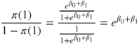
Where does the logistic regression curve come from? Consider the conditional mean of Y given X = x, denoted as ![]() . This is the expected value of the response variable for a given value of the predictor. Recall that, in linear regression, the response variable is considered to be a random variable defined as
. This is the expected value of the response variable for a given value of the predictor. Recall that, in linear regression, the response variable is considered to be a random variable defined as ![]() . Now, as the error term
. Now, as the error term ![]() has mean zero, we then obtain
has mean zero, we then obtain ![]() for linear regression, with possible values extending over the entire real number line.
for linear regression, with possible values extending over the entire real number line.
For simplicity, denote the conditional mean ![]() as
as ![]() . Then, the conditional mean for logistic regression takes on a different form from that of linear regression. Specifically,
. Then, the conditional mean for logistic regression takes on a different form from that of linear regression. Specifically,
Curves of the form in equation (13.1) are called sigmoidal because they are S-shaped, and therefore nonlinear. Statisticians have chosen the logistic distribution to model dichotomous data because of its flexibility and interpretability. The minimum for ![]() is obtained at
is obtained at ![]() , and the maximum for
, and the maximum for ![]() is obtained at
is obtained at ![]() . Thus,
. Thus, ![]() is of a form that may be interpreted as a probability, with
is of a form that may be interpreted as a probability, with ![]() . That is,
. That is, ![]() may be interpreted as the probability that the positive outcome (e.g., disease) is present for records with
may be interpreted as the probability that the positive outcome (e.g., disease) is present for records with ![]() , and
, and ![]() may be interpreted as the probability that the positive outcome is absent for such records.
may be interpreted as the probability that the positive outcome is absent for such records.
Linear regression models assume that ![]() , where the error term
, where the error term ![]() is normally distributed with mean zero and constant variance. The model assumption for logistic regression is different. As the response is dichotomous, the errors can take only one of two possible forms: If
is normally distributed with mean zero and constant variance. The model assumption for logistic regression is different. As the response is dichotomous, the errors can take only one of two possible forms: If ![]() (e.g., disease is present), which occurs with probability
(e.g., disease is present), which occurs with probability ![]() (the probability that the response is positive), then
(the probability that the response is positive), then ![]() , the vertical distance between the data point
, the vertical distance between the data point ![]() and the curve
and the curve ![]() directly below it, for
directly below it, for ![]() . However, if
. However, if ![]() (e.g., disease is absent), which occurs with probability
(e.g., disease is absent), which occurs with probability ![]() (the probability that the response is negative), then
(the probability that the response is negative), then ![]() , the vertical distance between the data point
, the vertical distance between the data point ![]() and the curve
and the curve ![]() directly above it, for
directly above it, for ![]() . Thus, the variance of
. Thus, the variance of ![]() is
is ![]() , which is the variance for a binomial distribution, and the response variable in logistic regression
, which is the variance for a binomial distribution, and the response variable in logistic regression ![]() is assumed to follow a binomial distribution with probability of success
is assumed to follow a binomial distribution with probability of success ![]() .
.
A useful transformation for logistic regression is the logit transformation, and it is given as follows:
The logit transformation ![]() exhibits several attractive properties of the linear regression model, such as its linearity, its continuity, and its range from negative to positive infinity.
exhibits several attractive properties of the linear regression model, such as its linearity, its continuity, and its range from negative to positive infinity.
13.2 Maximum Likelihood Estimation
One of the most attractive properties of linear regression is that closed-form solutions for the optimal values of the regression coefficients may be obtained, courtesy of the least-squares method. Unfortunately, no such closed-form solution exists for estimating logistic regression coefficients. Thus, we must turn to maximum-likelihood estimation, which finds estimates of the parameters for which the likelihood of observing the observed data is maximized.
The likelihood function ![]() is a function of the parameters
is a function of the parameters ![]() that expresses the probability of the observed data, x. By finding the values of
that expresses the probability of the observed data, x. By finding the values of ![]() , which maximize
, which maximize ![]() , we thereby uncover the maximum-likelihood estimators, the parameter values most favored by the observed data.
, we thereby uncover the maximum-likelihood estimators, the parameter values most favored by the observed data.
The probability of a positive response given the data is ![]() , and the probability of a negative response given the data is given by
, and the probability of a negative response given the data is given by ![]() . Then, observations where the response is positive,
. Then, observations where the response is positive, ![]() , will contribute probability
, will contribute probability ![]() to the likelihood, while observations where the response is negative,
to the likelihood, while observations where the response is negative, ![]() , will contribute probability
, will contribute probability ![]() to the likelihood. Thus, as
to the likelihood. Thus, as ![]() or 1, the contribution to the likelihood of the ith observation may be expressed as
or 1, the contribution to the likelihood of the ith observation may be expressed as ![]() . The assumption that the observations are independent allows us to express the likelihood function
. The assumption that the observations are independent allows us to express the likelihood function ![]() as the product of the individual terms:
as the product of the individual terms:
The log-likelihood ![]() is computationally more tractable:
is computationally more tractable:
The maximum-likelihood estimators may be found by differentiating ![]() with respect to each parameter, and setting the resulting forms equal to zero. Unfortunately, unlike linear regression, closed-form solutions for these differentiations are not available. Therefore, other methods must be applied, such as iterative weighted least squares (see McCullagh and Nelder2).
with respect to each parameter, and setting the resulting forms equal to zero. Unfortunately, unlike linear regression, closed-form solutions for these differentiations are not available. Therefore, other methods must be applied, such as iterative weighted least squares (see McCullagh and Nelder2).
13.3 Interpreting Logistic Regression Output
Let us examine the results of the logistic regression of disease on age, shown in Table 13.2. The coefficients, that is, the maximum-likelihood estimates of the unknown parameters ![]() and
and ![]() , are given as
, are given as ![]() and
and ![]() . Thus,
. Thus, ![]() is estimated as
is estimated as
with the estimated logit
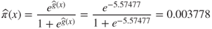
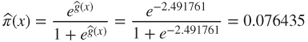
These equations may then be used to estimate the probability that the disease is present in a particular patient, given the patient's age. For example, for a 50-year-old patient, we have
and
Thus, the estimated probability that a 50-year-old patient has the disease is 26%, and the estimated probability that the disease is not present is 100% − 26% = 74%.
Table 13.2 Logistic regression of disease on age, results from minitab
 |
However, for a 72-year-old patient, we have
and
The estimated probability that a 72-year-old patient has the disease is 61%, and the estimated probability that the disease is not present is 39%.
13.4 Inference: Are the Predictors Significant?
Recall from simple linear regression that the regression model was considered significant if mean square regression (MSR) was large compared to mean squared error (MSE). The MSR is a measure of the improvement in estimating the response when we include the predictor, as compared to ignoring the predictor. If the predictor variable is helpful for estimating the value of the response variable, then MSR will be large, the test statistic ![]() will also be large, and the linear regression model will be considered significant.
will also be large, and the linear regression model will be considered significant.
Significance of the coefficients in logistic regression is determined analogously. Essentially, we examine whether the model that includes a particular predictor provides a substantially better fit to the response variable than a model that does not include this predictor.
Define the saturated model to be the model that contains as many parameters as data points, such as a simple linear regression model with only two data points. Clearly, the saturated model predicts the response variable perfectly, and there is no prediction error. We may then look on the observed values of the response variable to be the predicted values from the saturated model. To compare the values predicted by our fitted model (with fewer parameters than data points) to predicted by the saturated the values model, we use the deviance (McCullagh and Nelder3), as defined here:
Here we have a ratio of two likelihoods, so that the resulting hypothesis test is called a likelihood ratio test. In order to generate a measure whose distribution is known, we must take ![]() . Denote the estimate of
. Denote the estimate of ![]() from the fitted model to be
from the fitted model to be ![]() . Then, for the logistic regression case, and using equation (13.2), we have deviance equal to:
. Then, for the logistic regression case, and using equation (13.2), we have deviance equal to:
The deviance represents the error left over in the model, after the predictors have been accounted for. As such it is analogous to the sum of squares error in linear regression.
The procedure for determining whether a particular predictor is significant is to find the deviance of the model without the predictor and subtract the deviance of the model with the predictor, thus:

Let ![]() and
and ![]() . Then, for the case of a single predictor only, we have:
. Then, for the case of a single predictor only, we have:

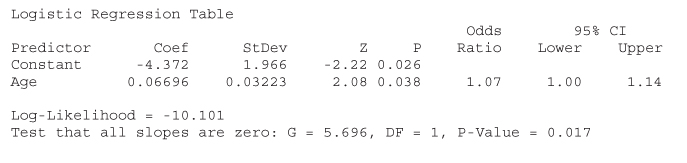
For the disease example, note from Table 13.2 that the log-likelihood is given as −10.101. Then,
as indicated in Table 13.2.
The test statistic ![]() follows a chi-square distribution with 1 degree of freedom (i.e.,
follows a chi-square distribution with 1 degree of freedom (i.e., ![]() ), assuming that the null hypothesis is true that
), assuming that the null hypothesis is true that ![]() . The resulting p-value for this hypothesis test is therefore
. The resulting p-value for this hypothesis test is therefore ![]() , as shown in Table 13.2. This fairly small p-value indicates that there is evidence that age is useful in predicting the presence of disease.
, as shown in Table 13.2. This fairly small p-value indicates that there is evidence that age is useful in predicting the presence of disease.
Another hypothesis test used to determine whether a particular predictor is significant is the Wald test (e.g., Rao4). Under the null hypothesis that ![]() , the ratio
, the ratio
follows a standard normal distribution, where SE refers to the standard error of the coefficient, as estimated from the data and reported by the software. Table 13.2 provides the coefficient estimate and the standard error as follows: ![]() and
and ![]() , giving us:
, giving us:
as reported under z for the coefficient age in Table 13.2. The p-value is then reported as ![]() . This p-value is also fairly small, although not as small as the likelihood ratio test, and therefore concurs in the significance of age for predicting disease.
. This p-value is also fairly small, although not as small as the likelihood ratio test, and therefore concurs in the significance of age for predicting disease.
We may construct ![]() confidence intervals for the logistic regression coefficients, as follows.
confidence intervals for the logistic regression coefficients, as follows.
where z represents the z-critical value associated with ![]() confidence.
confidence.
In our example, a 95% confidence interval for the slope ![]() could be found thus:
could be found thus:

As zero is not included in this interval, we can conclude with 95% confidence that ![]() , and that therefore the variable age is significant.
, and that therefore the variable age is significant.
The above results may be extended from the simple (one predictor) logistic regression model to the multiple (many predictors) logistic regression model. (See Hosmer and Lemeshow5 for details.)
13.5 Odds Ratio and Relative Risk
Recall from simple linear regression that the slope coefficient ![]() was interpreted as the change in the response variable for every unit increase in the predictor. The slope coefficient
was interpreted as the change in the response variable for every unit increase in the predictor. The slope coefficient ![]() is interpreted analogously in logistic regression, but through the logit function. That is, the slope coefficient
is interpreted analogously in logistic regression, but through the logit function. That is, the slope coefficient ![]() may be interpreted as the change in the value of the logit for a unit increase in the value of the predictor. In other words,
may be interpreted as the change in the value of the logit for a unit increase in the value of the predictor. In other words,
In this section, we discuss the interpretation of ![]() in simple logistic regression for the following three cases:
in simple logistic regression for the following three cases:
- A dichotomous predictor
- A polychotomous predictor
- A continuous predictor.
To facilitate our interpretation, we need to consider the concept of odds. Odds may be defined as the probability that an event occurs divided by the probability that the event does not occur. For example, earlier we found that the estimated probability that a 72-year-old patient has the disease is 61%, and the estimated probability that the 72-year-old patient does not have the disease is 39%. Thus, the odds of a 72-year-old patient having the disease equal ![]() . We also found that the estimated probabilities of a 50-year-old patient having or not having the disease are 26% and 74%, respectively, providing odds for the 50-year-old patient to be
. We also found that the estimated probabilities of a 50-year-old patient having or not having the disease are 26% and 74%, respectively, providing odds for the 50-year-old patient to be ![]() .
.
Note that when the event is more likely than not to occur, then ![]() ; when the event is less likely than not to occur, then
; when the event is less likely than not to occur, then ![]() ; and when the event is just as likely as not to occur, then
; and when the event is just as likely as not to occur, then ![]() . Note also that the concept of odds differs from the concept of probability, because probability ranges from zero to one while odds can range from zero to infinity. Odds indicate how much more likely it is that an event occurred compared to it is not occurring.
. Note also that the concept of odds differs from the concept of probability, because probability ranges from zero to one while odds can range from zero to infinity. Odds indicate how much more likely it is that an event occurred compared to it is not occurring.
In binary logistic regression with a dichotomous predictor, the odds that the response variable occurred (y = 1) for records with x = 1 can be denoted as:
Correspondingly, the odds that the response variable occurred for records with x = 0 can be denoted as:

The odds ratio (OR) is defined as the odds that the response variable occurred for records with x = 1 divided by the odds that the response variable occurred for records with x = 0. That is,

The OR is sometimes used to estimate the relative risk, defined as the probability that the response occurs for x = 1 divided by the probability that the response occurs for x = 0. That is,
For the OR to be an accurate estimate of the relative risk, we must have ![]() , which we obtain when the probability that the response occurs is small, for both x = 1 and x = 0.
, which we obtain when the probability that the response occurs is small, for both x = 1 and x = 0.
The OR has come into widespread use in the research community, because of the above simply expressed relationship between the OR and the slope coefficient. For example, if a clinical trial reports that the OR for endometrial cancer among ever-users and never-users of estrogen replacement therapy is 5.0, then this may be interpreted as meaning that ever-users of estrogen replacement therapy are five times more likely to develop endometrial cancer than are never-users. However, this interpretation is valid only when ![]() .
.
13.6 Interpreting Logistic Regression for a Dichotomous Predictor
| Recall the churn data set, where we were interested in predicting whether a customer would leave the cell phone company's service (churn), based on a set of predictor variables. For this simple logistic regression example, assume that the only predictor available is Voice Mail Plan, a flag variable indicating membership in the plan. |  |
The cross-tabulation of churn by Voice Mail Plan membership is shown in Table 13.3.
Table 13.3 Cross-tabulation of churn by membership in the voice mail plan
| VMail = No x = 0 | VMail = Yes x = 1 | Total | |
| Churn = False y = 0 |
2008 | 842 | 2850 |
| Churn = True y = 1 |
403 | 80 | 483 |
| Total | 2411 | 922 | 3333 |
The likelihood function is then given by:
Note that we may use the entries from Table 13.3 to construct the odds and the OR directly.
- Odds of those with Voice Mail Plan churning =

- Odds of those without Voice Mail Plan churning =
 , and
, and
That is, the odds of churning for those with the Voice Mail Plan is only 0.47 as large as the odds of churning for those without the Voice Mail Plan. Note that the OR can also be calculated as the following cross product:
The logistic regression can then be performed, with the results shown in Table 13.4.
Table 13.4 Results of logistic regression of churn on voice mail plan
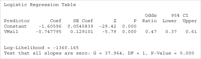 |
First, note that the OR reported by Minitab equals 0.47, the same value we found using the cell counts directly. Next, equation (13.3) tells us that ![]() . We verify this by noting that
. We verify this by noting that ![]() , so that
, so that ![]() .
.
Here we have ![]() and
and ![]() . So, the probability of churning for a customer belonging
. So, the probability of churning for a customer belonging ![]() or not belonging
or not belonging ![]() to the voice mail plan is estimated as:
to the voice mail plan is estimated as:
with the estimated logit:
For a customer belonging to the plan, we estimate his or her probability of churning:
and
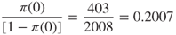
So, the estimated probability that a customer who belongs to the voice mail plan will churn is only 8.68%, which is less than the overall proportion of churners in the data set, 14.5%, indicating that belonging to the voice mail plan protects against churn. Also, this probability could have been found directly from Table 13.3, ![]() .
.
For a customer not belonging to the voice mail plan, we estimate the probability of churning:
and
This probability is slightly higher than the overall proportion of churners in the data set, 14.5%, indicating that not belonging to the voice mail may be slightly indicative of churning. This probability could also have been found directly from Table 13.3, ![]() .
.
Next, we apply the Wald test for the significance of the parameter for voice mail plan. We have ![]() , and
, and ![]() , giving us:
, giving us:
as reported under z for the coefficient Voice Mail Plan in Table 13.4. The p-value is ![]() , which is strongly significant. There is strong evidence that the Voice Mail Plan variable is useful for predicting the churn.
, which is strongly significant. There is strong evidence that the Voice Mail Plan variable is useful for predicting the churn.
A ![]() confidence interval for the OR may be found thus:
confidence interval for the OR may be found thus:
where ![]() represents
represents ![]() .
.
Thus, here we have a 95% confidence interval for the OR given by:

as reported in Table 13.4. Thus, we are 95% confident that the OR for churning among voice mail plan members and nonmembers lies between 0.37 and 0.61. As the interval does not include ![]() , the relationship is significant with 95% confidence.
, the relationship is significant with 95% confidence.
We can use the cell entries to estimate the standard error of the coefficients directly, as follows (result from Bishop, Feinberg, and Holland6). The standard error for the logistic regression coefficient ![]() for Voice Mail Plan is estimated as follows:
for Voice Mail Plan is estimated as follows:
In this churn example, the voice mail members were coded as 1 and the nonmembers coded as 0. This is an example of reference cell coding, where the reference cell refers to the category coded as zero. ORs are then calculated as the comparison of the members relative to the nonmembers, that is, with reference to the nonmembers.
In general, for variables coded as a and b rather than 0 and 1, we have:

So an estimate of the OR in this case is given by:
which becomes ![]() when
when ![]() and
and ![]() .
.
13.7 Interpreting Logistic Regression for a Polychotomous Predictor
For the churn data set, suppose we categorize the customer service calls variable into a new variable CSC as follows:
- Zero or one customer service calls: CSC = Low
- Two or three customer service calls: CSC = Medium
- Four or more customer service calls: CSC = High.
Then, CSC is a trichotomous predictor. How will logistic regression handle this? First, the analyst will need to code the data set using indicator (dummy) variables and reference cell coding. Suppose we choose CSC = Low to be our reference cell. Then we assign the indicator variable values to two new indicator variables CSC_Med and CSC_Hi, given in Table 13.5. Each record will have assigned to it a value of zero or one for each of CSC_Med and CSC_Hi. For example, a customer with 1 customer service call will have values CSC_Med = 0 and CSC_Hi = 0, a customer with three customer service calls will have CSC_Med = 1 and CSC_Hi = 0, and a customer with seven customer service calls will have CSC_Med = 0 and CSC_Hi = 1.
Table 13.5 Reference cell encoding for customer service calls indicator variables
| CSC_Med | CSC_Hi | |
| Low (0–1 calls) | 0 | 0 |
| Medium (2–3 calls) | 1 | 0 |
| High ( |
0 | 1 |
Table 13.6 shows a cross-tabulation of churn by CSC.
Table 13.6 Cross-tabulation of churn by CSC
| CSC = Low | CSC = Medium | CSC = High | Total | |
| Churn = False y = 0 |
1664 | 1057 | 129 | 2850 |
| Churn = True y = 1 |
214 | 131 | 138 | 483 |
| Total | 1878 | 1188 | 267 | 3333 |
Using CSC = Low as the reference class, we can calculate the ORs using the cross products as follows:
- For CSC = Medium, we have
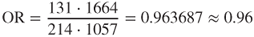 ;
; - For CSC = High, we have
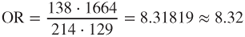 .
.
The logistic regression is then performed, with the results shown in Table 13.7.
Table 13.7 Results of logistic regression of churn on CSC
 |
Note that the ORs reported by Minitab are the same that we found using the cell counts directly. We verify the ORs given in Table 13.7 using equation (13.3):
- CSC_Med:

- CSC_Hi:

Here we have ![]() ,
, ![]() , and
, and ![]() . So, the probability of churning is estimated as:
. So, the probability of churning is estimated as:
with the estimated logit:
For a customer with low customer service calls, we estimate his or her probability of churning:
and
So, the estimated probability that a customer with low numbers of customer service calls will churn is 11.4%, which is less than the overall proportion of churners in the data set, 14.5%, indicating that such customers churn somewhat less frequently than the overall group. Also, this probability could have been found directly from Table 13.6, ![]() .
.
For a customer with medium customer service calls, the probability of churn is estimated as:
and
The estimated probability that a customer with medium numbers of customer service calls will churn is 11.0%, which is about the same as that for customers with low numbers of customer service calls. The analyst may consider collapsing the distinction between CSC_Med and CSC_Low. This probability could have been found directly from Table 13.6, ![]() .
.
For a customer with high customer service calls, the probability of churn is estimated as:
and
Thus, customers with high levels of customer service calls have a much higher estimated probability of churn, over 51%, which is more than triple the overall churn rate. Clearly, the company needs to flag customers who make four or more customer service calls, and intervene with them before they leave the company's service. This probability could also have been found directly from Table 13.6, ![]() .
.
Applying the Wald test for the significance of the CSC_Med parameter, we have ![]() , and
, and ![]() , giving us:
, giving us:
as reported under z for the coefficient CSC_Med in Table 13.7. The p-value is ![]() , which is not significant. There is no evidence that the CSC_Med versus CSC_Low distinction is useful for predicting the churn.
, which is not significant. There is no evidence that the CSC_Med versus CSC_Low distinction is useful for predicting the churn.
For the CSC_Hi parameter, we have ![]() , and
, and ![]() , giving us:
, giving us:
as shown for the coefficient CSC_Hi in Table 13.7. The p-value, ![]() , indicates that there is strong evidence that the distinction CSC_Hi versus CSC_Low is useful for predicting the churn.
, indicates that there is strong evidence that the distinction CSC_Hi versus CSC_Low is useful for predicting the churn.
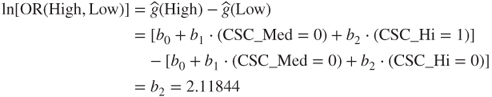
Examining Table 13.7, note that the ORs for both CSC = Medium and CSC = High are equal to those we calculated using the cell counts directly. Also note that the logistic regression coefficients for the indicator variables are equal to the natural log of their respective ORs:
For example, the natural log of the OR of CSC_High to CSC_Low can be derived using equation (13.4) as follows:
Similarly, the natural log of the OR of CSC_Medium to CSC_Low is given by:

Just as for the dichotomous case, we may use the cell entries to estimate the standard error of the coefficients directly. For example, the standard error for the logistic regression coefficient ![]() for CSC_Med is estimated as follows:
for CSC_Med is estimated as follows:
Also similar to the dichotomous case, we may calculate ![]() confidence intervals for the ORs, for the ith predictor, as follows:
confidence intervals for the ORs, for the ith predictor, as follows:
For example, a 95% confidence interval for the OR between CSC_Hi and CSC_Low is given by:

as reported in Table 13.7. We are 95% confident that the OR for churning for customers with high customer service calls compared to customers with low customer service calls lies between 6.29 and 11.0. As the interval does not include ![]() , the relationship is significant with 95% confidence.
, the relationship is significant with 95% confidence.
However, consider the 95% confidence interval for the OR between CSC_Med and CSC_Low:

as reported in Table 13.7. We are 95% confident that the OR for churning for customers with medium customer service calls compared to customers with low customer service calls lies between 0.77 and 1.21. As this interval does include ![]() , then the relationship is not significant with 95% confidence. Depending on other modeling factors, the analyst may consider collapsing CSC_Med and CSC_Low into a single category.
, then the relationship is not significant with 95% confidence. Depending on other modeling factors, the analyst may consider collapsing CSC_Med and CSC_Low into a single category.
13.8 Interpreting Logistic Regression for a Continuous Predictor
Our first example of predicting the presence of disease based on age was an instance of using a continuous predictor in logistic regression. Here we present another example, based on the churn data set. Suppose we are interested in predicting churn based on a single continuous variable, Day Minutes.
We first examine an individual value plot of the day minute usage among churners and non-churners, provided in Figure 13.2.

Figure 13.2 Churners have slightly higher mean day minutes usage.
The plot seems to indicate that churners have slightly higher mean day minute usage than non-churners, meaning that heavier usage may be a predictor of churn. We verify this using the descriptive statistics given in Table 13.8. The mean and five-number-summary for the churn = true customers indicates higher day minutes usage than for the churn = false customers, supporting the observation from Figure 13.2.
Table 13.8 Descriptive statistics for day minutes by churn
 |
Is this difference significant? A two-sample t-test is carried out, with the null hypothesis being that there is no difference in true mean day minute usage between churners and non-churners. The results are shown in Table 13.9.
Table 13.9 Results of two-sample t-test for day minutes by churn
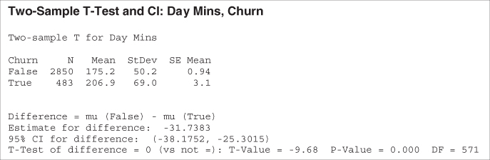 |
The resulting t-statistic is −9.68, with a p-value rounding to zero, representing strong significance. That is, the null hypothesis that there is no difference in true mean day minute usage between churners and non-churners is strongly rejected.
Let us reiterate our word of caution about carrying out inference in data mining problems, or indeed in any problem where the sample size is very large. Most statistical tests become very sensitive at very large sample sizes, rejecting the null hypothesis for tiny effects. The analyst needs to understand that, just because the effect is found to be statistically significant because of the huge sample size, it does not necessarily follow that the effect is of practical significance. The analyst should keep in mind the constraints and desiderata of the business or research problem, seek confluence of results from a variety of models, and always retain a clear eye for the interpretability of the model and the applicability of the model to the original problem.
Note that the t-test does not give us an idea of how an increase in Day Minutes affects the odds that a customer will churn. Neither does the t-test provide a method for finding the probability that a particular customer will churn, based on the customer's day minutes usage. To learn this, we must turn to logistic regression, which we now carry out, with the results given in Table 13.10.
Table 13.10 Results of logistic regression of churn on day minutes
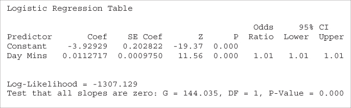 |
First, we verify the relationship between the OR for Day Minutes and its coefficient. ![]() , as shown in Table 13.10. We discuss interpreting this value a bit later. In this example we have
, as shown in Table 13.10. We discuss interpreting this value a bit later. In this example we have ![]() and
and ![]() . Thus, the probability of churning
. Thus, the probability of churning ![]() for a customer with a given number of day minutes is estimated as:
for a customer with a given number of day minutes is estimated as:
with the estimated logit:
For a customer with 100 day minutes, we can estimate his or her probability of churning:
and
Thus, the estimated probability that a customer with 100 day minutes will churn is less than 6%. This is less than the overall proportion of churners in the data set, 14.5%, indicating that low day minutes somehow protects against churn.
However, for a customer with 300 day minutes, we have
and
The estimated probability that a customer with 300 day minutes will churn is over 36%, which is more than twice the overall proportion of churners in the data set, indicating that heavy-use customers have a higher propensity to churn.
The deviance difference G for this example is given by:

as indicated in Table 13.10.
The p-value for the chi-square test for G, under the assumption that the null hypothesis is true ![]() , is given by
, is given by ![]() , as shown in Table 13.10. Thus, the logistic regression concludes that there is strong evidence that Day Minutes is useful in predicting churn.
, as shown in Table 13.10. Thus, the logistic regression concludes that there is strong evidence that Day Minutes is useful in predicting churn.
Applying the Wald test for the significance of the Day Minutes parameter, we have ![]() , and
, and ![]() , giving us:
, giving us:
as shown in Table 13.10. The associated p-value of ![]() , using
, using ![]() , indicates strong evidence for the usefulness of the Day Minutes variable for predicting churn.
, indicates strong evidence for the usefulness of the Day Minutes variable for predicting churn.
Examining Table 13.10, note that the coefficient for Day Minutes is equal to the natural log of its OR:
Also, this coefficient may be derived as follows, similarly to equation (13.4), as follows:

This derivation provides us with the interpretation of the value for ![]() . That is,
. That is, ![]() represents the estimated change in the log OR, for a unit increase in the predictor. In this example,
represents the estimated change in the log OR, for a unit increase in the predictor. In this example, ![]() , which means that, for every additional day minute that the customer uses, the log OR for churning increases by 0.0112717.
, which means that, for every additional day minute that the customer uses, the log OR for churning increases by 0.0112717.
The value for the OR we found above, ![]() , may be interpreted as the odds of a customer with x + 1 minutes churning compared to the odds of a customer with x minutes churning. For example, a customer with 201 minutes is about 1.01 times as likely to churn as compared to a customer with 200 minutes.
, may be interpreted as the odds of a customer with x + 1 minutes churning compared to the odds of a customer with x minutes churning. For example, a customer with 201 minutes is about 1.01 times as likely to churn as compared to a customer with 200 minutes.
This unit-increase interpretation may be of limited usefulness, because the analyst may prefer to interpret the results using a different scale, such as 10 or 60 min, or even (conceivably) 1 s. We therefore generalize the interpretation of the logistic regression coefficient as follows:
This result can be seen to follow from the substitution of ![]() for
for ![]() in equation (13.5):
in equation (13.5):

For example, let ![]() , so that we are interested in the change in the log OR for an increase of 60 day minutes of cell phone usage. This increase would be estimated as
, so that we are interested in the change in the log OR for an increase of 60 day minutes of cell phone usage. This increase would be estimated as ![]() . Consider a customer A, who had 60 more day minutes than customer B. Then we would estimate the OR for customer A to churn compared to customer B to be
. Consider a customer A, who had 60 more day minutes than customer B. Then we would estimate the OR for customer A to churn compared to customer B to be ![]() . That is, an increase of 60 day minutes nearly doubles the odds that a customer will churn.
. That is, an increase of 60 day minutes nearly doubles the odds that a customer will churn.
Similar to the categorical predictor case, we may calculate ![]() confidence intervals for the ORs, as follows:
confidence intervals for the ORs, as follows:
For example, a 95% confidence interval for the OR for Day Minutes is given by:

as reported in Table 13.10. We are 95% confident that the OR for churning for customers with one additional day minute lies between 1.0094 and 1.0133. As the interval does not include ![]() , the relationship is significant with 95% confidence.
, the relationship is significant with 95% confidence.
Confidence intervals may also be found for the OR for the ith predictor, when there is a change in c units in the predictor, as follows:
For example, earlier we estimated the increase in the OR, when the day minutes increased by c = 60 minutes, to be 1.97. The 99% confidence interval associated with this estimate is given by:
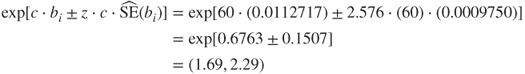
So, we are 99% confident that an increase of 60 day minutes will increase the OR of churning by a factor of between 1.69 and 2.29.
13.9 Assumption of Linearity
Now, if the logit is not linear in the continuous variables, then there may be problems with the application of estimates and confidence intervals for the OR. The reason is that the estimated OR is constant across the range of the predictor. For example, the estimated OR of 1.01 is the same for every unit increase of Day Minutes, whether it is the 23rd minute or the 323rd minute. The same is true of the estimated OR for the increase of 60 day minutes; the estimated OR of 1.97 is the same whether we are referring to the 0–60 min timeframe or the 55–115 min timeframe, and so on.
Such an assumption of constant OR is not always warranted. For example, suppose we performed a logistic regression of churn on Customer Service Calls (the original variable, not the set of indicator variables), which takes values 0–9. The results are shown in Table 13.11.
Table 13.11 Questionable results of logistic regression of churn on customer service calls
 |
The estimated OR of 1.49 indicates that the OR for churning increases by this factor for every additional customer service call that is made. We would therefore expect that a plot of Customer Service Calls with a churn overlay would form a fairly regular steplike pattern. However, consider Figure 13.3, which shows a normalized histogram of Customer Service Calls with a churn overlay. (The normalization makes each rectangle the same length, thereby increasing the contrast, at the expense of information about bin size.) Darker portions indicate the proportion of customers who churn.

Figure 13.3 Normalized histogram of customer service calls with churn overlay.
Note that we do not encounter a gradual step-down pattern as we proceed left to right. Instead, there is a single rather dramatic discontinuity at four customer service calls. This is the pattern we uncovered earlier when we performed binning on customer service calls, and found that those with three or fewer calls had a much different propensity to churn than did customers with four or more.
Specifically, the results in Table 13.11 assert that, for example, moving from zero to one customer service calls increases the OR by a factor of 1.49. This is not the case, as fewer customers with one call churn than do those with zero calls. For example, Table 13.12 shows the counts of customers churning and not churning for the 10 values of Customer Service Calls, along with the estimated OR for the one additional customer service call. For example, the estimated OR for moving from zero to one call is 0.76, which means that churning is less likely for those making one call than it is for those making none. The discontinuity at the fourth call is represented by the OR of 7.39, meaning that a customer making his or her fourth call is more than seven times as likely to churn as a customer who has made three calls.
Table 13.12 Customer service calls by churn, with estimated odds ratios
| Customer Service Calls | ||||||||||
| 0 | 1 | 2 | 3 | 4 | 5 | 6 | 7 | 8 | 9 | |
| Churn = False | 605 | 1059 | 672 | 385 | 90 | 26 | 8 | 4 | 1 | 0 |
| Churn = True | 92 | 122 | 87 | 44 | 76 | 40 | 14 | 5 | 1 | 2 |
| Odds ratio | — | 0.76 | 1.12 | 0.88 | 7.39 | 1.82 | 1.14 | 0.71 | 0.8 | Undefined |
Note that the OR of 1.49, which results from an inappropriate application of logistic regression, is nowhere reflected in the actual data. If the analyst wishes to include customer service calls in the analysis (and it should be included), then certain accommodations to nonlinearity must be made, such as the use of indicator variables (see the polychotomous example) or the use of higher order terms (e.g., ![]() ). Note the undefined OR for the 9 column that contains a zero cell. We discuss the zero-cell problem below.
). Note the undefined OR for the 9 column that contains a zero cell. We discuss the zero-cell problem below.
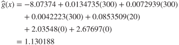
For another example of the problem of nonlinearity, we turn to the Adult data set,7 which was extracted from data provided by the US Census Bureau. The task is to find the set of demographic characteristics that can best predict whether or not the individual has an income of over $50,000 per year. We restrict our attention to the derived variable, capnet, which equals the capital gains amount minus the capital losses, expressed in dollars. The naïve application of logistic regression of income on capnet provides the results shown in Table 13.13.
Table 13.13 Results of questionable logistic regression of income on capnet
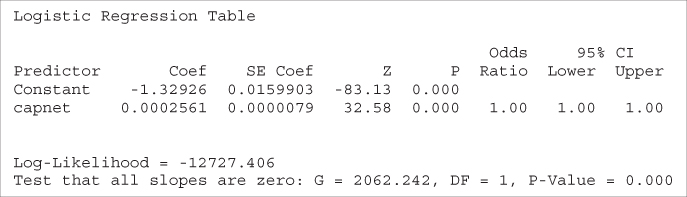 |
The OR for the capnet variable is reported as 1.00, with both endpoints of the confidence interval also reported as 1.00. Do we conclude from this that capnet is not significant? And if so, then how do we resolve the apparent contradiction with the strongly significant Z-test p-value of approximately zero?
Actually, of course, there is no contradiction. The problem lies in the fact that the OR results are reported only to two decimal places. More detailed 95% confidence intervals are provided here:

Thus, the 95% confidence interval for the capnet variable does not include the null value of ![]() , indicating that this variable is in fact significant. Why is such precision needed? Because capnet is measured in dollars. One additional dollar in capital gains, for example, would presumably not increase the probability of a high income very dramatically. Hence, the tiny but significant OR. (Of course, requesting more decimal points in the output would have uncovered similar results.)
, indicating that this variable is in fact significant. Why is such precision needed? Because capnet is measured in dollars. One additional dollar in capital gains, for example, would presumably not increase the probability of a high income very dramatically. Hence, the tiny but significant OR. (Of course, requesting more decimal points in the output would have uncovered similar results.)
However, nearly 87% of the records have zero capnet (neither capital gains nor capital losses). What effect would this have on the linearity assumption? Table 13.14 provides the income level counts for a possible categorization of the capnet variable.
Table 13.14 Income level counts for categories of capnet
| Income | Capnet Categories | |||||||
| Loss | None | Gain <$3000 | Gain ≥$3000 | |||||
| ≤$50,000 | 574 | 49.7% | 17,635 | 81.0% | 370 | 100% | 437 | 25.6% |
| >$50,000 | 582 | 50.3% | 4133 | 19.0% | 0 | 0% | 1269 | 74.4% |
| Total | 1156 | 21,768 | 370 | 1706 | ||||
Note that high income is associated with either capnet loss or capnet gain ≥$3000, while low income is associated with capnet none or capnet gain <$3000. Such relationships are incompatible with the assumption of linearity. We would therefore like to rerun the logistic regression analysis, this time using the capnet categorization shown in Table 13.14.
13.10 Zero-Cell Problem
Unfortunately, we are now faced with a new problem, the presence of a zero-count cell in the cross-classification table. There are no records of individuals in the data set with income greater than $50,000 and capnet gain less than $3000. Zero cells play havoc with the logistic regression solution, causing instability in the analysis and leading to possibly unreliable results.
Rather than omitting the “gain < $3000” category, we may try to collapse the categories or redefine them somehow, in order to find some records for the zero cell. In this example, we will try to redefine the class limits for the two capnet gains categories, which will have the added benefit of finding a better balance of records in these categories. The new class boundaries and cross-classification is shown in Table 13.15.
Table 13.15 Income level counts for categories of capnet, new categorization
| Income | Capnet Categories | |||||||
| Loss | None | Gain < $5000 | Gain ≥$5000 | |||||
| ≤$50,000 | 574 | 49.7% | 17,635 | 81.0% | 685 | 83.0% | 122 | 9.8% |
| >$50,000 | 582 | 50.3% | 4133 | 19.0% | 140 | 17.0% | 1129 | 90.2% |
| Total | 1156 | 21,768 | 370 | 1706 | ||||
The logistic regression of income on the newly categorized capnet has results that are shown in Table 13.16.
Table 13.16 Results from logistic regression of income on categorized capnet
 |
The reference category is zero capnet. The category of gain <$5000 is not significant, because its proportions of high and low income are quite similar to those of zero capnet, as shown in Table 13.15. The categories of loss and gain ≥$5000 are both significant, but at different orders of magnitude. Individuals showing a capital loss are 4.33 times as likely to have high income than zero capnet individuals, while people showing a capnet gain of at least $5000 are nearly 40 times more likely to have high income than the reference category.
The variability among these results reinforces the assertion that the relationship between income and capnet is nonlinear, and that naïve insertion of the capnet variable into a logistic regression would be faulty.
For a person showing a capnet loss, we can estimate his or her probability of having an income above $50,000. First the logit:
with probability:
So, the probability that a person with a capnet loss has an income above $50,000 is about 50–50. Also, we can estimate the probability that a person showing a capnet gain of at least $5000 will have an income above $50,000. The logit is:
and the probability is:
Note that these probabilities are the same as could be found using the cell counts in Table 13.15. It is similar for a person with a capnet gain of under $5000. However, this category was found to be not significant. What, then, should be our estimate of the probability that a person with a small capnet gain will have high income?
Should we use the estimate provided by the cell counts and the logistic regression (probability = 17%), even though it was found to be not significant? The answer is no, not for formal estimation. To use nonsignificant variables for estimation increases the chances that the estimation will not be generalizable. That is, the generalizability (and hence, usefulness) of the estimation will be reduced.
Now, under certain circumstances, such as a cross-validated (see validating the logistic regression, below) analysis, where all subsamples concur that the variable is nearly significant, then the analyst may annotate the estimation with a note that there may be some evidence for using this variable in the estimation. However, in general, retain for estimation and prediction purposes only those variables that are significant. Thus, in this case, we would estimate the probability that a person with a small capnet gain will have high income as follows:
with probability:
which is the same as the probability that a person with zero capnet will have high income.
13.11 Multiple Logistic Regression
Thus far, we have examined logistic regression using only one variable at a time. However, very few data mining data sets are restricted to one variable! We therefore turn to multiple logistic regression, in which more than one predictor variable is used to classify the binary response variable.
Returning to the churn data set, we examine whether a relationship exists between churn and the following set of predictors.
- International Plan, a flag variable
- Voice Mail Plan, a flag variable
- CSC-Hi, a flag variable indicating whether or not a customer had high (
 ) level of customer services calls
 - Account length, continuous
- Day Minutes, continuous
- Evening Minutes, continuous
- Night Minutes, continuous
- International Minutes, continuous.
The results are provided in Table 13.17.
Table 13.17 Results of multiple logistic regression of churn on several variables
 |
First, note that the overall regression is significant, as shown by the p-value of approximately zero for the G-statistic. Therefore, the overall model is useful for classifying churn.
However, not all variables contained in the model need necessarily be useful. Examine the p-values for the (Wald) z-statistics for each of the predictors. All p-values are small except one, indicating that there is evidence that each predictor belongs in the model, except Account Length, the standardized customer account length. The Wald z-statistic for account length is 0.56, with a large p-value of 0.578, indicating that this variable is not useful for classifying churn. Further, the 95% confidence interval for the OR includes 1.0, reinforcing the conclusion that Account Length does not belong in the model.
Therefore, we now omit Account Length from the model, and proceed to run the logistic regression again with the remaining variables. The results are shown in Table 13.18. Comparing Table 13.18 to Table 13.17, we see that the omission of Account Length has barely affected the remaining analysis. All remaining variables are considered significant, and retained in the model.
Table 13.18 Results of multiple logistic regression after omitting account length
 |
The positive coefficients indicate predictors for which an increase in the value of the predictor is associated with an increase in the probability of churning. Similarly, negative coefficients indicate predictors associated with reducing the probability of churn. Unit increases for each of the minutes variables are associated with an increase in the probability of churn, as well as membership in the International Plan, and customers with high levels of customer service calls. Only membership in the Voice Mail Plan reduces the probability of churn.
Table 13.18 provides the estimated logit:

where Intl Plan = Yes, VMail Plan = Yes, and CSC-Hi = 1 represent indicator (dummy) variables. Then, using
we may estimate the probability that a particular customer will churn, given various values for the predictor variables. We will estimate the probability of churn for the following customers:
- A low usage customer belonging to no plans with few calls to customer service.
- A moderate usage customer belonging to no plans with few calls to customer service.
- A high usage customer belonging to the International Plan but not the Voice Mail Plan, with many calls to customer service.
- A high usage customer belonging to the Voice Mail Plan but not the International Plan, with few calls to customer service.
- A low usage customer belonging to no plans with few calls to customer service. This customer has 100 minutes for each of day, evening, and night minutes, and no international minutes. The logit looks like:

The probability that customer (1) will churn is therefore:
That is, a customer with low usage, belonging to no plans, and making few customer service calls has less than a 1% chance of churning.
- A moderate usage customer belonging to no plans with few calls to customer service. This customer has 180 day minutes, 200 evening and night minutes, and 10 international minutes, each number near the average for the category. Here is the logit:

The probability that customer (2) will churn is:
A customer with moderate usage, belonging to no plans, and making few customer service calls still has less than an 8% probability of churning.
- A high usage customer belonging to the International Plan but not the Voice Mail Plan, with many calls to customer service. This customer has 300 day, evening, and night minutes, and 20 international minutes. The logit is:

Thus, the probability that customer (3) will churn is:

High usage customers, belonging to the International Plan but not the Voice Mail Plan, and with many calls to customer service, have as astonishing 99.71% probability of churning. The company needs to deploy interventions for these types of customers as soon as possible, to avoid the loss of these customers to other carriers.
- A high usage customer belonging to the Voice Mail Plan but not the International Plan, with few calls to customer service. This customer also has 300 day, evening, and night minutes, and 20 international minutes. The logit is:

- Hence, the probability that customer (4) will churn is:

- This type of customer has over a 50% probability of churning, which is more than three times the 14.5% overall churn rate.
- A low usage customer belonging to no plans with few calls to customer service. This customer has 100 minutes for each of day, evening, and night minutes, and no international minutes. The logit looks like:
For data that are missing one or more indicator variable values, it would not be appropriate to simply ignore these missing variables when making an estimation. For example, suppose for customer (4), we had no information regarding membership in the Voice Mail Plan. If we then ignored the Voice Mail Plan variable when forming the estimate, then we would get the following logit:
Note that this is the same value for ![]() that we would obtain for a customer who was known to not be a member of the Voice Mail Plan. To estimate the probability of a customer whose Voice Mail Plan membership was unknown using this logit would be incorrect. This logit would instead provide the probability of a customer who did not have the Voice Mail Plan, but was otherwise similar to customer (4), as follows:
that we would obtain for a customer who was known to not be a member of the Voice Mail Plan. To estimate the probability of a customer whose Voice Mail Plan membership was unknown using this logit would be incorrect. This logit would instead provide the probability of a customer who did not have the Voice Mail Plan, but was otherwise similar to customer (4), as follows:
Such a customer would have a churn probability of about 76%.
13.12 Introducing Higher Order Terms to Handle Nonlinearity
We illustrate how to check the assumption of linearity in multiple logistic regression by returning to the Adult data set. For this example, we shall use only the following variables:
- Age
- Education-num
- Hours-per-week
- Capnet (=capital gain – capital loss)
- Marital-status
- Sex
- Income: the target variable, binary, either ≤$50,000 or >$50,000.
The three “Married” categories in marital-status in the raw data were collapsed into a single “Married” category. A normalized histogram of age with an overlay of the target variable income is shown in Figure 13.4.
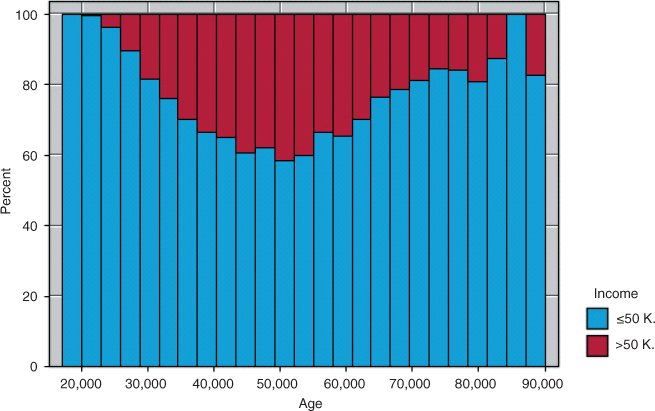
Figure 13.4 Normalized histogram of Age with Income overlay shows quadratic relationship.
The darker bands indicate the proportion of high incomes. Clearly, this proportion increases until about age 52, after which it begins to drop again. This behavior is nonlinear and should not be naively modeled as such in the logistic regression. Suppose, for example, that we went ahead and performed a logistic regression of income on the singleton predictor age. The results are shown in Table 13.19.
Table 13.19 Results of naïve application of logistic regression of income on age
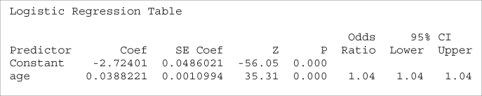 |
Table 13.19 shows that the predictor age is significant, with an estimated OR of 1.04. Recall that the interpretation of this OR is as follows: that the odds of having high income for someone of age ![]() are 1.04 times higher than for someone of age
are 1.04 times higher than for someone of age ![]() .
.
Now consider this interpretation in light of Figure 13.4. The OR of 1.04 is clearly inappropriate for the subset of subjects older than 50 or so. This is because the logistic regression assumes linearity, while the actual relationship is nonlinear.
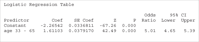
There are a couple of approaches we could take to alleviate this problem. First, we could use indicator variables as we did earlier. Here, we use an indicator variable age 33–65, where all records falling in this range are coded as 1 and all other records coded as 0. This coding was used because the higher incomes were found in the histogram to fall within this range. The resulting logistic regression is shown in Table 13.20. The OR is 5.01, indicating that persons between 33 and 65 years of age are about five times more likely to have high income than persons outside this age range.
Table 13.20 Logistic regression of income on age 33–65
 |
An alternative modeling method would be to directly model the quadratic behavior of the relationship by introducing an ![]() (age-squared) variable. The logistic regression results are shown in Table 13.21.
(age-squared) variable. The logistic regression results are shown in Table 13.21.
Table 13.21 Introducing a quadratic term age2 to model the nonlinearity of age
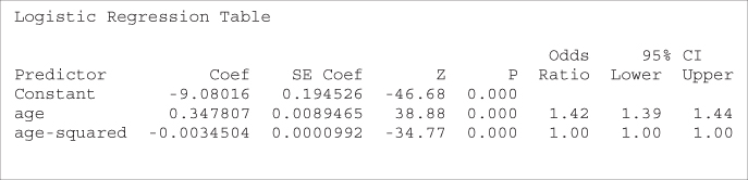 |
The OR for the age variable has increased from the value of 1.04, previously determined, to 1.42. For the age2 term, the OR and the endpoints of the confidence interval are reported as 1.00, but this is only due to rounding. We use the fact that ![]() to find the more accurate estimate of the OR as
to find the more accurate estimate of the OR as ![]() . Also, the 95% confidence interval is given by
. Also, the 95% confidence interval is given by

which concurs with the p-value regarding the significance of the term.
The age2 term acts as a kind of penalty function, reducing the probability of high income for records with high age. We examine the behavior of the age and age2 terms working together by estimating the probability that each of the following people will have incomes greater than $50,000:
- A 30-year-old person
- A 50-year-old person
- A 70-year-old person.
We have the estimated logit:
which has the following values for our three individuals:
Note that the logit is greatest for the 50-year-old, which models the behavior seen in Figure 13.4. Then, the estimated probability of having an income greater than $50,000 is then found for our three people:

The probabilities that the 30-year-old, 50-year-old, and 70-year-old have an income greater than $50,000 are 14.79%, 42.17%, and 16.24%, respectively. This is compared to the overall proportion of the 25,000 records in the training set that have income greater than $50,000, which is ![]() .
.
One benefit of using the quadratic term (together with the original age variable) rather than the indicator variable is that the quadratic term is continuous, and can presumably provide tighter estimates for a variety of ages. For example, the indicator variable age 33–65 categorizes all records into two classes, so that a 20-year-old is binned together with a 32-year-old, and the model (all other factors held constant) generates the same probability of high income for the 20-year-old as the 32-year-old. The quadratic term, however, will provide a higher probability of high income for the 32-year-old than the 20-year-old (see exercises).
Next, we turn to the education-num variable, which indicates the number of years of education the subject has had. The relationship between income and education-num is shown in Figure 13.5.
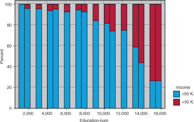
Figure 13.5 Normalized histogram of education-num with income overlay.
The pattern shown in Figure 13.5 is also quadratic, although perhaps not as manifestly so as in Figure 13.4. As education increases, the proportion of subjects having high income also increases, but not at a linear rate. Until eighth grade or so, the proportion increases slowly, and then more quickly as education level increases. Therefore, modeling the relationship between income and education level as strictly linear would be an error; we again need to introduce a quadratic term.
Note that, for age, the coefficient of the quadratic term age2 was negative, representing a downward influence for very high ages. For education-num, however, the proportion of high incomes is highest for the highest levels of income, so that we would expect a positive coefficient for the quadratic term education2. The results of a logistic regression run on education-num and ![]() are shown in Table 13.22.
are shown in Table 13.22.
Table 13.22 Results from logistic regression of income on education-num and education2
 |
As expected, the coefficient for ![]() is positive. However, note that the variable education-num is not significant, because it has a large p-value, and the confidence interval contains 1.0. We therefore omit education-num from the analysis and perform a logistic regression of income on
is positive. However, note that the variable education-num is not significant, because it has a large p-value, and the confidence interval contains 1.0. We therefore omit education-num from the analysis and perform a logistic regression of income on ![]() alone, with results shown in Table 13.23.
alone, with results shown in Table 13.23.
Table 13.23 Results from logistic regression of income on education2 alone
 |
Here, the ![]() term is significant, and we have
term is significant, and we have ![]() , with the 95% confidence interval given by:
, with the 95% confidence interval given by:

We estimate the probability that persons with the following years of education will have incomes greater than $50,000:
- 12 years of education
- 16 years of education.
The estimated logit:
has the following values:
Then, we can find the estimated probability of having an income greater than $50,000 as:
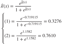
The probabilities that people with 12 years and 16 years of education will have an income greater than $50,000 are 32.76% and 76.10%, respectively. Evidently, for this population, it pays to stay in school.
Finally, we examine the variable hours-per-week, which represents the number of hours worked per week for the subject. The normalized histogram is shown in Figure 13.6.
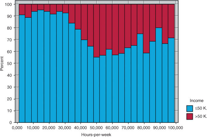
Figure 13.6 Normalized histogram of hours-per-week with income overlay.
In Figure 13.6, we certainly find nonlinearity. A quadratic term would seem indicated by the records up to 50 h per week. However, at about 50 h per week, the pattern changes, so that the overall curvature is that of a backwards S-curve. Such a pattern is indicative of the need for a cubic term, where the cube of the original variable is introduced. We therefore do so here, introducing ![]() , and performing the logistic regression of income on hours-per-week,
, and performing the logistic regression of income on hours-per-week, ![]() , and
, and ![]() , with the results shown in Table 13.24.
, with the results shown in Table 13.24.
Table 13.24 Results from logistic regression of income on hours-per-week, hours2, and hours3
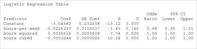 |
Note that the original variable, hours-per-week, is no longer significant. We rerun the analysis, including only ![]() and
and ![]() , with the results shown in Table 13.25. Both the
, with the results shown in Table 13.25. Both the ![]() and
and ![]() terms are significant. Analysis and interpretation of these results is left to the exercises.
terms are significant. Analysis and interpretation of these results is left to the exercises.
Table 13.25 Results from logistic regression of income on hours2 and hours3
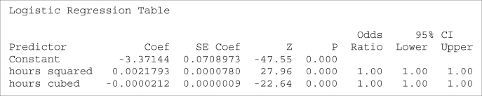 |
Putting all the previous results from this section together, we construct a logistic regression model for predicting income based on the following variables:


- Capnet-cat
- Marital-status
- Sex.
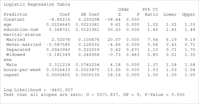
The results, provided in Table 13.26, are analyzed and interpreted in the exercises.
Table 13.26 Results from multiple logistic regression of income
 |
13.13 Validating the Logistic Regression Model
Hosmer and Lebeshow8 provide details for assessing the fit of a logistic regression model, including goodness-of-fit statistics and model diagnostics. Here, however, we investigate validation of the logistic regression model through the traditional method of a hold-out sample.
The training data set of 25,000 records was partitioned randomly into two data sets, training set A of 12,450 records and training set B of 12,550 records. Training set A has 2953 records (23.72%) with income greater than $50,000, while training set B has 3031 (24.15%) such records. Therefore, we cannot expect that the parameter estimates and ORs for the two data sets will be exactly the same. Indicator variables are provided for marital status and sex. The reference categories (where all indicators equal zero) are divorced and female, respectively. The logistic regression results for training sets A and B are provided in Tables 13.27 and 13.28, respectively.
Table 13.27 Logistic regression results for training set A
 |
Table 13.28 Logistic regression results for training set B
 |
Note that, for both data sets, all parameters are significant (as shown by the Wald-Z p-values) except the separated and widowed indicator variables for marital status. Overall, the coefficient values are fairly close to each other, except those with high variability, such as male and separated.
The estimated logit for training sets A and B are:


For each of these logits, we will estimate the probability that each of the following types of people have incomes over $50,000:
- A 50-year-old married male with 20 years of education working 40 hours per week with a capnet of $500.
- A 50-year-old married male with 16 years of education working 40 hours per week with no capital gains or losses.
- A 35-year-old divorced female with 12 years of education working 30 hours per week with no capital gains or losses.
-
For the 50-year-old married male with 20 years of education working 40 hours per week with a capnet of $500, we have the following logits for training sets A and B:

Thus, the estimated probability that this type of person will have an income exceeding $50,000 is for each data set:

That is, the estimated probability that a 50-year-old married male with 20 years of education working 40 hours per week with a capnet of $500 will have an income exceeding $50,000 is 96.66%, as reported by both data sets with a difference of only 0.000002 between them. If sound, then the similarity of these estimated probabilities shows strong evidence for the validation of the logistic regression.
Unfortunately, these estimates are not sound, because they represent extrapolation on the education variable, whose maximum value in this data set is only 16 years. Therefore, these estimates should not be used in general, and should certainly not be used for model validation.
- For the 50-year-old married male with 16 years of education working 40 hours per week with a capnet of $500, the logits look like this:

- The estimated probability that a 50-year-old married male with 16 years of education working 40 hours per week with a capnet of $500 will have an income exceeding $50,000 is therefore for each data set:

- That is, the estimated probability that such a person will have an income greater than $50,000 is reported by models based on both data sets to be about 87%. There is a difference of only 0.0026 between the point estimates, which may be considered small, although, of course, what constitutes small depends on the particular research problem, and other factors.
- For the 35-year-old divorced female with 12 years of education working 30 hours per week with no capital gains or losses, we have the following logits:
 Therefore, for each data set, the estimated probability that this type of person will have an income exceeding $50,000 is:

- That is, the estimated probability that a 35-year-old divorced female with 12 years of education working 30 hours per week with no capital gains or losses will have an income greater than $50,000 is reported by models based on both data sets to be between 6.3% and 6.5%. There is a difference of only 0.00158 between the point estimates, which is slightly better (i.e., smaller) than the estimate for the 50-year-old male.
13.14 WEKA: Hands-On Analysis Using Logistic Regression
In this exercise, a logistic regression model is built using Waikato Environment for Knowledge Analysis (WEKA's) Logistic class. A modified version of the cereals data set is used as input, where the RATING field is discretized by mapping records with values greater than 42 to “High,” while those less than or equal to 42 become “Low.” This way, our model is used to classify a cereal as having either a “High” or “Low” nutritional rating. Our data set consists of the three numeric predictor fields PROTEIN, SODIUM, and FIBER.
The data set is split into separate training and test files. The training file cereals_train.arff consists of 24 instances and is used to train our logistic regression model. The file is balanced 50–50 where half the instances take on class value “High,” while the other half have the value “Low.” The mean values for the predictor fields PROTEIN, SODIUM, and FIBER are 2.667, 146.875, and 2.458, respectively. The complete training file is shown in Table 13.29.
Table 13.29 ARFFTraining Filecereals_train.arff
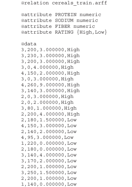 |
Our training and test files are both represented in ARFF format, which is WEKA's standard method of representing the instances and attributes found in data sets. The keyword relation indicates the name for the file, which is followed by a block defining each attribute in the data set. Notice that the three predictor fields are defined as type numeric, whereas the target variable RATING is categorical. The data section lists each instance, which corresponds to a specific cereal. For example, the first line in the data section describes a cereal having PROTEIN = 3, SODIUM = 200, FIBER = 3.0, and RATING = High.
Let us load the training file and build the Logistic model.
- Click Explorer from the WEKA GUI Chooser dialog.
- On the Preprocess tab, press Open file and specify the path to the training file, cereals_train.arff.
The WEKA Explorer Panel displays several characteristics of the training file as shown in Figure 13.7. The three predictor attributes and class variable are shown on the attributes pane (left). Statistics for PROTEIN, including range (1–4), mean (2.667), and standard deviation (0.868) are shown on the selected attribute pane (right). The status bar at the bottom of the panel tells us WEKA loaded the file successfully.
- Next, select the Classify tab.
- Under Classifier, press the Choose button.
- Select Classifiers → Functions → Logistic from the navigation hierarchy.
- In our modeling experiment, we have separate training and test sets; therefore, under Test options, choose the Use training set option.
- Click Start to build the model.
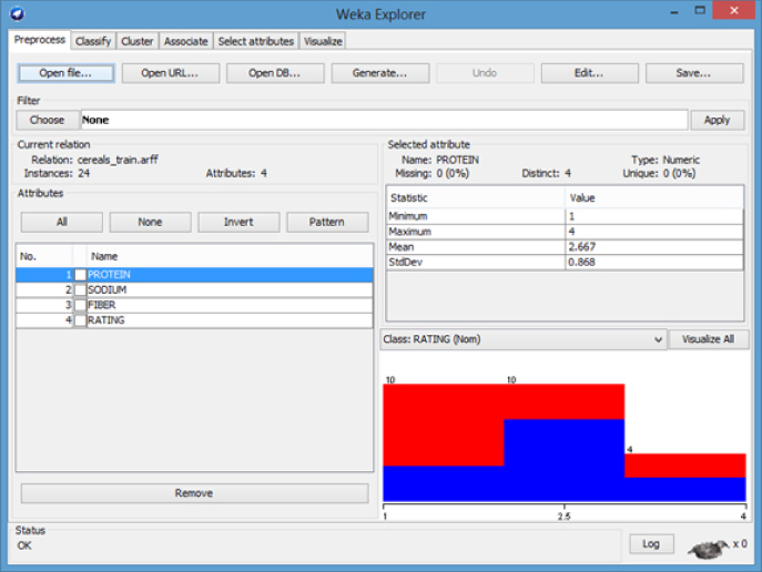
Figure 13.7 WEKA explorer panel: preprocess tab.
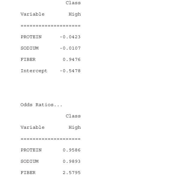
WEKA creates the logistic regression model and reports results in the Classifier output window. Although the results (not shown) indicate that the classification accuracy of the model, as measured against the training set, is ![]() , we are interested in using the model to classify the unseen data found in the test set. The ORs and values for the regression coefficients
, we are interested in using the model to classify the unseen data found in the test set. The ORs and values for the regression coefficients ![]() ,
, ![]() ,
, ![]() , and
, and ![]() are also reported by the model as shown in Table 13.30. We will revisit these values shortly, but first let us evaluate our model against the test set.
are also reported by the model as shown in Table 13.30. We will revisit these values shortly, but first let us evaluate our model against the test set.
Table 13.30 Logistic regression coefficients
 |
- Under Test options, choose Supplied test set. Click Set.
- Click Open file, specify the path to the test file, cereals_test.arff. Close the Test Instances dialog.
- Next, click the More options button.
- Check the Output text predictions on test set option. Click OK.
- Click the Start button to evaluate the model against the test set.
Again, the results appear in the Classifier output window; however, now the output shows that the logistic regression model has classified ![]() of the instances in the test set correctly. In addition, the model now reports the actual predictions, and probabilities by which it classified each instance, as shown in Table 13.31.
of the instances in the test set correctly. In addition, the model now reports the actual predictions, and probabilities by which it classified each instance, as shown in Table 13.31.
Table 13.31 Logistic regression test set predictions
 |
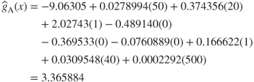
For example, the first instance is incorrectly predicted (classified) to be “Low” with probability 0.567. The plus (+) symbol in error column indicates this classification is incorrect according to the maximum (*0.567) probability. Let us compute the estimated logit ![]() for this instance according to the coefficients found in Table 13.30.
for this instance according to the coefficients found in Table 13.30.
However, we first examine the test file cereals_test.arff and determine the first record contains the attribute-value pairs PROTEIN = 4, SODIUM = 135, FIBER = 2.0, and RATING = High. Therefore, the estimated logit equals:
It follows that,
Therefore, the estimated probability equals about 43.4% that a cereal with protein (4 g), sodium (135 mg), and fiber (2 g) is of high nutritional value. Note that WEKA reports this same probability (except for slight rounding variations) for the first instance in Table 13.31. It follows that the model estimates a probability equal to ![]() that this cereal has a low nutritional rating. Therefore, based on the higher probability, the model incorrectly classified the record as “Low.”
that this cereal has a low nutritional rating. Therefore, based on the higher probability, the model incorrectly classified the record as “Low.”
Table 13.31 also shows reports of the ORs for the three continuous predictors. For example, the OR for PROTEIN is ![]() . This is interpreted as the odds of a cereal with x + 1 grams of protein being of high nutritional value, as compared to a cereal with x grams of protein being highly nutritious.
. This is interpreted as the odds of a cereal with x + 1 grams of protein being of high nutritional value, as compared to a cereal with x grams of protein being highly nutritious.
R References
- R Core Team. R: A Language and Environment for Statistical Computing. Vienna, Austria: R Foundation for Statistical Computing; 2012. 3-900051-07-0, http://www.R-project.org/. Accessed 2014 Oct 5.
Exercises
Clarifying the Concepts
1. Indicate whether the following statements are true or false. If the statement is false, alter it so that the statement becomes true.
- Logistic regression refers to methods for describing the relationship between a categorical response variable and a set of categorical predictor variables.
- Logistic regression assumes the relationship between the predictor and the response is nonlinear.
 may be interpreted as a probability.
- Logistic regression models assume that the error term
 is normally distributed with mean zero and constant variance.
 - In logistic regression, closed-form solutions for the optimal values of the regression coefficients may be obtained.
- The saturated model predicts the response variable perfectly.
- The deviance represents the total variability in the response.
- Encoding a trichotomous predictor requires only two indicator variables.
- The t-test provides a method for finding the response probabilities.
- The interpretation of the logistic regression coefficient for a continuous predictor may be extended from the usual unit increase to an increase of any arbitrary amount.
- The estimated OR is constant across the range of the predictor.
2. By hand, derive the logit result ![]() .
.
3. Explain what is meant by maximum-likelihood estimation and maximum-likelihood estimators.
4. Explain clearly how the slope coefficient ![]() , and its estimate
, and its estimate ![]() , may be interpreted in logistic regression. Provide at least two examples, using both a categorical and a continuous predictor.
, may be interpreted in logistic regression. Provide at least two examples, using both a categorical and a continuous predictor.
5. What are odds? What is the difference between odds and probability?
6. What is the definition of the odds ratio? What is the relationship between the odds ratio and the slope coefficient ![]() ? For what quantity is the odds ratio sometimes used as an estimate?
? For what quantity is the odds ratio sometimes used as an estimate?
7. Describe how we determine the statistical significance of the odds ratio, using a confidence interval.
8. If the difference between a particular indicator variable and the reference category is not significant, then what should the analyst consider doing?
9. Discuss the role of statistical inference with respect to the huge sample sizes prevalent in data mining.
10. Discuss the assumption that the odds ratio is constant across the range of the predictor, with respect to various types of relationships between the predictor and the response. Provide modeling options for when this assumption may not be reflected in the data.
11. Discuss the use of predictors that turn out to be nonsignificant in estimating the response. When might this be appropriate, if at all? Why would this not be appropriate in general?
12. Explain why, for data that are missing one or more indicator variable values, it would not be appropriate to simply ignore these missing variables when making an estimation. Provide options for the data analyst in this case.
Working with the Data
For Exercises 13–18, use the following information. The logistic regression output shown in Table 13.32 refers to the breast cancer data set. This data set was collected by Dr. William H. Wohlberg from the University of Wisconsin Hospitals, Madison. Ten numeric predictors are used to predict the class of malignant breast cancer tumor (class = 1), as opposed to a benign tumor (class = 0).
Table 13.32 Logistic regression results for Exercises 13
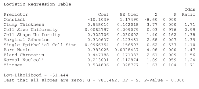 |
13. What is the value of the deviance difference? Is the overall logistic regression significant? How can you tell? What does it mean to say that the overall logistic regression is significant?
14. Without reference to inferential significance, express the form of the logit.
15. Which variables do not appear to be significant predictors of breast tumor class? How can you tell?
16. Discuss whether the variables you cited in Exercise 15 should be used in predicting the class of tumor with a new unseen data set.
17. Discuss how you should handle the variables with p-values around 0.05, 0.10, or 0.15.
18. Explain what will happen to the deviance difference if we rerun the model, dropping the nonsignificant variables. Work by analogy with the linear regression case.
For Exercises 19–24, use the following information. Continuing from the previous exercises, the logistic regression for the breast cancer data set was run again, this time dropping the cell size uniformity and single epithelial cell size variables, but retaining all the others. The logistic regression output shown in Table 13.33 contains the results.
Table 13.33 Logistic regression results for Exercises 19–24
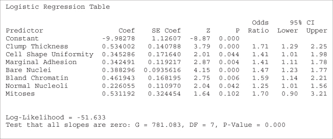 |
19. Explain why the deviance difference fell, but only by a small amount.
20. Did you drop cell shape uniformity in the previous exercise? Are you surprised that the variable is now a significant predictor? Discuss the importance of retaining variables of borderline significance in the early stages of model building.
21. Assume that our level of significance is 0.11. Express the logit, using all significant variables.
22. Find the probability that a tumor is malignant, given the following:
- The values for all predictors are at the minimum (1).
- The values for all predictors are at a moderate level (5).
- The values for all predictors are at the maximum (10).
23. Calculate the 95% confidence intervals for the following predictor coefficients.
- Clump thickness
- Mitoses
- Comment as to the evidence provided by the confidence interval for the mitoses coefficient regarding its significance.
24. Clearly interpret the value of the coefficients for the following predictors:
- Bland chromatin
- Normal nucleoli
Hands-On Analysis
For Exercises 25–37, use the adult data set.
25. Construct the logistic regression model developed in the text, with the ![]() term and the indicator variable age 33–65.
term and the indicator variable age 33–65.
Verify that using the quadratic term provides a higher estimate of the probability of high income for the 32-year-old than the 20-year-old.
Use Table 13.25 for Exercises 26–28.
26. Find the form of the estimated logit.
27. Find the probability of high income for someone working 30, 40, 50, and 60 hours per week.
28. Construct and interpret a 95% confidence interval for each coefficient.
Use Table 13.26 for Exercises 29–31.
29. Consider the results from Table 13.26. Construct the logistic regression model that produced these results.
30. For indicator categories that are not significant, collapse the categories with the reference category. (How are you handling the category with the 0.083 p-value?) Rerun the logistic regression with these collapsed categories.
Use the results from your rerunning of the logistic regression for Exercises 31–34.
31. Find the estimated logit.
32. Construct and interpret 95% confidence intervals for the coefficients for age, sex-male, and educ-squared. Verify that these predictors belong in the model.
33. Find the probability of high income for a 20-year-old single female with 12 years education working 20 hours per week with no capital gains or losses.
34. Find the probability of high income for a 50-year-old married male with 16 years education working 40 hours per week with capital gains of $6000.
35. Open the data set, German, which is provided on the textbook website. The data set consists of 20 predictors, both continuous and categorical, and a single response variable, indicating whether the individual record represents a good or bad credit risk. The predictors are as follows, with amounts in Deutsche marks (DM):
- Status of existing checking account
- Duration in months
- Credit history
- Loan purpose
- Credit amount
- Savings account/bonds
- Presently employed since
- Payment as percentage of disposable income
- Personal status and gender
- Other debtors/guarantors
- Present residence since
- Property
- Age
- Other installment plans
- Housing
- Number of existing credits at this bank
- Job
- Number of people being liable to provide maintenance for
- Telephone
- Foreign worker.
More information is available about this data set from the textbook website. Construct the best logistic regression model you can, using as many of the methods we learned in this chapter as possible. Provide strong interpretive support for your model, including explanations of derived variables, indicator variables, and so on.
36. Open the breast cancer data set. Investigate, for each significant predictor, whether the linearity assumption is warranted. If not, ameliorate the situation using the methods discussed in this chapter.
37. Recall the WEKA Logistic example for classifying cereals as either high or low. Compute the probability that the fourth instance from the test set is classified either high or low. Does your probability match that produced by WEKA?