
Chapter 5
Semi-Markov Models
5.1. Introduction
After almost 50 years of research on Markovian dependence—research rich in theoretical and applied results, at the International congress of mathematics held in Amsterdam in 1954, P. Lévy and W. L. Smith introduced a new class of stochastic processes, called by both authors semi-Markov processes. It seems that it was K. L. Chung who had suggested the idea to P. Lévy. Also in 1954, Takács introduced the same type of stochastic process and used it to counter theory applied to the registering of elementary particles.
Starting from that moment, the theory of semi-Markov processes has known an important development, with various fields of application. Nowadays, there is a large literature on this topic ([BAL 79, ÇIN 69b, ÇIN 69a, GIH 74, HAR 76, HOW 64, KOR 82, KOR 93, LIM 01, PYK 61a, PYK 61b, SIL 80, BAR 08], etc.) and, as far as we are concerned, we only want to provide here a general presentation of semi-Markov processes.
Semi-Markov processes are a natural generalization of Markov processes. Markov processes and renewal processes are particular cases of semi-Markov processes. For such a process, its future evolution depends only on the time elapsed from its last transition, and the sojourn time in any state depends only on the present state and on the next state to be visited. As opposed to Markov processes where the sojourn time in a state is exponentially distributed, the sojourn time distribution of a semi-Markov process can be any arbitrary distribution on ![]() +. This chapter is concerned with finite state minimal semi-Markov processes associated with Markov renewal processes. Therefore, we do not have to take into account instantaneous states and, on the other hand, the sojourn times of the process form almost surely a dense set in
+. This chapter is concerned with finite state minimal semi-Markov processes associated with Markov renewal processes. Therefore, we do not have to take into account instantaneous states and, on the other hand, the sojourn times of the process form almost surely a dense set in ![]() .
.
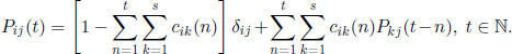
In this chapter we define the Markov renewal process and derive the main associated characteristics necessary for applications. We are concerned only with regular Markov renewal processes with discrete state space. This usually suffices for solving practical problems that we encounter in fields like reliability, reservoir systems, queueing systems, etc.
5.2. Markov renewal processes
5.2.1. Definitions
Let E be an infinite countable set and an ![]() E-valued jump process. Let 0 = T0 ≤ T1≤ ··· ≤ Tn ≤ Tn+1≤ ··· be the jump times of Z and J0, J1, J2, … be the successively visited states of Z. Note that T0 could also take positive values.
E-valued jump process. Let 0 = T0 ≤ T1≤ ··· ≤ Tn ≤ Tn+1≤ ··· be the jump times of Z and J0, J1, J2, … be the successively visited states of Z. Note that T0 could also take positive values.
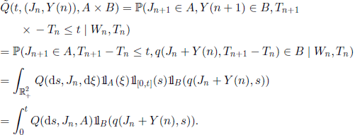
DEFINITION 5.1.– The stochastic process ((Jn, Tn), n ∈ ![]() ) is said to be a Markov renewal process (MRP), with state space E, if it satisfies almost surely the equality
) is said to be a Markov renewal process (MRP), with state space E, if it satisfies almost surely the equality
![]()
for all j ∈ E and t ∈ ![]() . In this case, Z is called a semi-Markov process (SMP).
. In this case, Z is called a semi-Markov process (SMP).
In fact, the process (Jn, Tn) is a Markov chain with state space E × ![]() and transition kernel Qij(t)
and transition kernel Qij(t)![]() , called semi-Markov kernel. It is easy to see that (Jn) is a Markov chain with state space E and transition probability
, called semi-Markov kernel. It is easy to see that (Jn) is a Markov chain with state space E and transition probability ![]() , called the embedded Markov chain (EMC) of the MRP. The semi-Markov chain Z is related to (Jn ,Tn) by
, called the embedded Markov chain (EMC) of the MRP. The semi-Markov chain Z is related to (Jn ,Tn) by
![]()
Note that a Markov process with state space E = ![]() and infinitesimal generator matrix A = (aij)i,j∈E is a special case of semi-Markov process with semi-Markov kernel
and infinitesimal generator matrix A = (aij)i,j∈E is a special case of semi-Markov process with semi-Markov kernel
![]()
where ![]() .
.
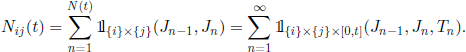
Let us also consider the sequence of r.v. Xn := Tn − Tn−1, n ≥ 1, the times between successive jumps, and the process ![]() + that counts the number of jumps of Z during the time interval (0, t], defined by N(t) := sup{n ≥ 0 | Tn ≤ t}. Let us also denote by Ni(t) the number of times the process Z passed to state i ∈ E up to time t. More precisely,
+ that counts the number of jumps of Z during the time interval (0, t], defined by N(t) := sup{n ≥ 0 | Tn ≤ t}. Let us also denote by Ni(t) the number of times the process Z passed to state i ∈ E up to time t. More precisely,
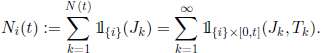
If we consider the renewal process ![]() , possible delayed, of successive passage times in state i, then Ni(t) is exactly the counting process of renewals associated with this renewal process. Let us denote by μii the mean recurrence time of
, possible delayed, of successive passage times in state i, then Ni(t) is exactly the counting process of renewals associated with this renewal process. Let us denote by μii the mean recurrence time of ![]() .
.
Let Q(t) = (Qij(t), i, j ∈ E), t ≥ 0, denote the semi-Markov kernel of Z. Then we can write
where ![]() is the conditional distribution function of the time between two successive jumps. Define also the sojourn time distribution function in state i, Hi(t) := Σj∈E Qij(t), and denote by mi, its mean value, which represents the mean sojourn time in state i of the process Z.
is the conditional distribution function of the time between two successive jumps. Define also the sojourn time distribution function in state i, Hi(t) := Σj∈E Qij(t), and denote by mi, its mean value, which represents the mean sojourn time in state i of the process Z.
Note that Hi is a distribution function, whereas Qij is a sub-distribution function (defective distribution function), i.e. Qij(∞) ≤ 1 and Hi(∞) = 1, with Qij(0−) = Hi(0−) = 0.
A special case of a semi-Markov process is obtained if Fij does not depend on j, i.e. Fij(t) = Fi(t) = Hi(t), and the semi-Markov kernel is
Another particular case of a semi-Markov process is obtained when Fij does not depend on i.
It is worth noticing that any semi-Markov process can be transformed in a process of the type [5.2], by considering the MRP (Jn, Jn+1, Tn)n≥0 with state space E × E. The semi-Markov kernel in this case is
where ![]() , with P(j,
, with P(j, ![]() ) = Qij(∞), the transition probability of the Markov chain (Jn, Jn+1)n≥0 and
) = Qij(∞), the transition probability of the Markov chain (Jn, Jn+1)n≥0 and ![]() Fij(t) the distribution function of the sojourn time in state (i,j), for all i, j, k,
Fij(t) the distribution function of the sojourn time in state (i,j), for all i, j, k, ![]() ∈ E and t ∈
∈ E and t ∈ ![]() .
.
For φ(i, t), i ∈ E, t ≥ 0, a real measurable function, the convolution of φ with Q is defined by
Let us also define the n-fold convolution of Q. For alli, j ∈ E
It is easy to prove by induction that
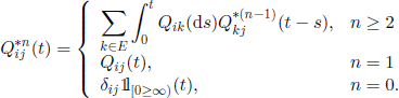
Let us introduce the Markov renewal function ψij(t), i, j ∈ E, t ≥ 0, defined by
Another important function is the semi-Markov transition function, defined by
![]()
which is the marginal distribution of the process.
DEFINITION 5.2.– The semi-Markov process Z is called regular if
![]()
for all t ≥ 0 and for all i ∈ E.
For any regular semi-Markov process we have, for all n ∈ ![]() , Tn < Tn+1 and Tn → ∞. In the following we consider only regular semi-Markov processes. The following result provides a regularity criterion for a semi-Markov process.
, Tn < Tn+1 and Tn → ∞. In the following we consider only regular semi-Markov processes. The following result provides a regularity criterion for a semi-Markov process.
THEOREM 5.3.– If there exist two constants, say α > 0 and β > 0, such that Hi(α) < 1 − β for any state i ∈ E, then the semi-Markov process is regular.
5.2.2. Markov renewal theory
Like the renewal equation on the real half-line x ≥ 0, the Markov renewal equation is a basic tool for the theory and the applications of semi-Markov processes.
The Markov renewal function introduced in [5.6] has the matrix expression
This can be equally written under the form
where I(t) = I (identity matrix) if t ≥ 0 and I(t) = 0, if t < 0. Equation [5.8] is a special case of what we will call a Markov renewal equation (MRE). The general form of a MRE is
where Θ(t) = (Θij(t), i, j ∈ E) and L(t) = (Lij(t), i, j ∈ E) are measurable matrix-valued functions, with Θij(t) = Lij(t) = 0 for t < 0. L(t) is a known matrix-valued function, whereas Θ(t) is unknown. We can equally write a vector version of equation [5.9], by considering the corresponding columns of the matrices Θ and L.
Let B be the space of all matrix-valued functions Θ(t), bounded on compact sets of ![]() is bounded on [0, ξ] for all ξ ∈
is bounded on [0, ξ] for all ξ ∈ ![]() .
.
THEOREM 5.4.– ([ÇIN 69a]). Equation [5.9] has a solution Θ belonging to B if and only if ψ * L belongs to B. Any solution Θ can be written under the form (t) = ψ * L(t) + C(t), where C satisfies equation C * L(t) Θ=C(t), C(t) ∈ B. A solution of (5.9) of the form Θ(t) = ψ * L(t) exists if one of the following conditions is satisfied:
1) The state space E is finite.
2) The EMC is irreducible and positive recurrent.
3) There exists t > 0 such that supi∈E; Hi(t) < 1.
4) Lij(t) is uniformly bounded in i for any j and t ∈ ![]() , and for any i there exists an a > 0 such that Hi(α) < 1 − β, β ∈ (0,1). If this is the case, the unique solution is uniformly bounded in i, for any j ∈ E and t > 0.
, and for any i there exists an a > 0 such that Hi(α) < 1 − β, β ∈ (0,1). If this is the case, the unique solution is uniformly bounded in i, for any j ∈ E and t > 0.
The following result is a first application of this theorem.
PROPOSITION 5.5.– The semi-Markov transition function P(t) = (Pij (t)) satisfies the MRE
![]()
which has the unique solution
provided that at least one of the conditions of Theorem 5.4 is satisfied. We have used the notation H(t) = diag(Hi(t)) and
![]()
EXAMPLE 5.6.– Let us consider an alternating renewal process defined by the distribution functions F for the working times and G for the failure times (repairing or replacement).
This process can be modeled by a two-state semi-Markov process with the semi-Markov kernel
![]()
for t ≥ 0.
Consequently, the semi-Markov transition function is given by
![]()
where M is the renewal function of the distribution function F * G, i.e.
![]()
5.3. First-passage times and state classification
Let ![]() , denote the family of random variables of the successive passage times to state j; so
, denote the family of random variables of the successive passage times to state j; so ![]() is the first-passage time to state j ∈ E and
is the first-passage time to state j ∈ E and ![]() is the distribution function of the first-passage time from state i to state j. For i = j we have
is the distribution function of the first-passage time from state i to state j. For i = j we have ![]() and
and ![]() is the distribution function of the time between two successive visits of state i.
is the distribution function of the time between two successive visits of state i.
We can write
and, for i ≠ j,
DEFINITION 5.7.– A MRP is said to be normal if ψ(0) < +∞. In this case, the semi-Markov transition matrix is also called normal.
A normal MRP is also regular.
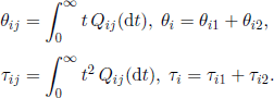
Let us consider a normal MRP with state space E and let μij = ![]() be the expected value of the first-passage time to state j, starting from i at time 0.
be the expected value of the first-passage time to state j, starting from i at time 0.
DEFINITION 5.8.–
1)We say that states i and j communicate if Gij(+∞)Gij(∞) > 0 or i = j. The communication is an equivalence relation.
2)A MRP is said to be irreducible if there is only one communication class.
3)A class C is said to be essential (or closed) if for any i ∈ C and t ≥ 0, we have Σj∈C Pij(t) = 1.
4)A state i is said to be recurrent if Gij(+∞) = 1 or ψii(+∞) = +∞. In the opposite case, the state i is said to be transient (ψii(+∞) < + ∞).
5)A state i is said to be null recurrent if it is recurrent and μii = ∞. The state is said to be positive recurrent if it is recurrent and μii < ∞.
6)A state i is said to be periodic of period h > 0 if Gii(·) is arithmetic, i.e. it has the distribution concentrated on (nh, n > 0). In this case, ψii(t) is constant on intervals of the type [nh, nh + h), with h the largest number with this property. In the opposite case, the state i is said to be aperiodic. Note that the notion of periodicity we introduced here is different from the periodicity of Markov chains.
5.3.1. Stationary distribution and asymptotic results
A basic tool in the asymptotic theory of semi-Markov processes is the Markov renewal theorem.
For any real function h(u) = (hi(u))i∈E we set ![]() for any u. We also let
for any u. We also let
![]()
where v = (vi,i ∈ E) is the stationary distribution of the EMC (Jn).
THEOREM 5.9.– If the EMC (Jn) is positive recurrent and 0 < m < 00 (ergodic process), then, for any i, j ∈ E, we have, for t → ∞:
1. ![]()
2. ![]()
3. ![]()
In the following we use again (see section 4.1) the notion of directly Riemann integrable function (DRI).
PROPOSITION 5.10.– A necessary and sufficient condition for a function g to be DRI is that
– g(t) ≥ 0 for all t ≥ 0;
– g(·) is non-increasing;
– ![]()
THEOREM 5.11.–
1. For any aperiodic state i ∈ E, if hi is a directly Riemann integrable function on ![]() , then, for t → ∞, we have
, then, for t → ∞, we have
![]()
2. For an irreducible and aperiodic MRP, if the functions (hi(u))i∈E are directly Riemann integrable, then, for t → ∞, we have
![]()
where v is a positive solution of vP = v.
From this theorem and the MRE [5.10] we obtain, for any ergodic MRP
and any j ∈ E, for t → ∞,
the limit (stationary) distribution of the semi-Markov process Z.
PROPOSITION 5.12.– We have:
1. ![]() .
.
2. ![]() .
.
It is worth noticing that the stationary distribution π of Z is not the same as the stationary distribution v of the EMC J. However, we have π = v if, for example, mi = a > 0 for all i ∈ E.
We will state now the central limit theorem of Pyke and Schaufele.
Let f be a measurable real application defined on E × E × ![]() . For all t ≥ 0 we define the functional Wf (t) by
. For all t ≥ 0 we define the functional Wf (t) by
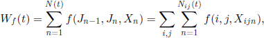
where Xijn is the nth sojourn time in state i, when the next state is j, and
Let
and

where s is the number of states of the process.
THEOREM 5.13.– (Law of large numbers of Pyke-Schaufele [PYK 64]). Under the hypothesis that the moments defined above exist, then
THEOREM 5.14.– (Central limit theorem of Pyke-Schaufele [PYK 64]). Under the hypothesis that the moments defined above exist, then
5.4. Reliability
Let us consider a system with temporal behavior described by a semi-Markov process Zt, t ≥ 0, with finite state space E, partitioned in two subsets, U = {1, 2,…, r} containing the functioning states and D = {r + 1,…, s} for the failure states. Let T be the lifetime of the system, i.e. the first-passage time of the process Zt to the failure states of the system.
The conditional and non-conditional reliability of a semi-Markov system, Ri(t) and R(t), can be written as
![]()
and
![]()
The reliability and availability functions of a semi-Markov system satisfy associated Markov renewal equations. For the reliability we have
We solve this MRE and obtain
![]()
where 1 = (1, …, 1)′ and α is the row vector of the initial distribution of the process.1
Similarly, for the availability we obtain
![]()
where e = (e1, …, es)′ is an s-dimensional column vector, with ei = 1, if i ∈ U, and ei, = 0, if i ∈ D.
Similarly, the maintainability can be written as
![]()
It is worth noticing that, for D a closed set, which means that the system is non-repairable, we have A(t) ≡ R(t). This is the reason why the availability is not used in survival analysis.
PROPOSITION 5.15.– The explicit expressions of the reliability, availability, and maintainability are:
Reliability
Availability
Maintainability
where Q(t) = (Qij(t), i,j ∈ E), t ≥ 0, is the semi-Markov kernel, Q00(t)is the restriction of Q(t) to U × U; HD = diag(H1, …, Hs), with Hi = ΣQij(t), and ![]() is the restriction of HD to U; P = Q(∞).
is the restriction of HD to U; P = Q(∞).
Integrating the MRE [5.17] over ![]() we obtain
we obtain
![]()
or, in matrix form,
![]()
where ![]() and m is the column vector of mean sojourn times in the states of the system,
and m is the column vector of mean sojourn times in the states of the system, ![]() , with m0 and m1 being the corresponding restrictions to U, respectively to D.
, with m0 and m1 being the corresponding restrictions to U, respectively to D.
From this equation we obtain the MTTF, and by an analogous approach, the MTTR. The MUT and MDT are obtained by replacing in the expressions of MTTF and MTTR, respectively, the initial distribution α (and its restrictions) by ![]() the probabilities of entering U and D when coming from D and U.
the probabilities of entering U and D when coming from D and U.
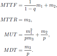
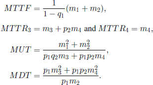
PROPOSITION 5.16.– (Mean times) The explicit expressions of the mean times are:
1) Mean time to failure, MTTF
2) Mean time to repair, MTTR
3) Mean up time (mean working time after repair), MUT
4) Mean down time (mean repair time after failure), MDT
The failure rate of a semi-Markov system is defined by
From this definition, assuming that the semi-Markov kernel Q is absolutely continuous with respect to the Lebesgue measure on ![]() , we obtain
, we obtain
where ![]() is the diagonal matrix of the derivatives of Hi(t), i ∈ U, i.e.
is the diagonal matrix of the derivatives of Hi(t), i ∈ U, i.e. ![]() .
.
The rate of occurrence of system failure (or intensity of the failure process) is an important reliability indicator. Let Nf(t),t ≥ 0, be the counting process of the number of transitions from U to D for a semi-Markov system, i.e. the number of system failures up to time t, and let ![]() be the mean number of failures up to time t. The rate of occurrence of failure (ROCOF) is the intensity of the process Nf(t), t ≥ 0, i.e. the derivative of the function ψf(t) with respect to t. In the exponential case, the ROCOF equals the failure rate. The following theorem provides an explicit expression of the ROCOF of a semi-Markov system.
be the mean number of failures up to time t. The rate of occurrence of failure (ROCOF) is the intensity of the process Nf(t), t ≥ 0, i.e. the derivative of the function ψf(t) with respect to t. In the exponential case, the ROCOF equals the failure rate. The following theorem provides an explicit expression of the ROCOF of a semi-Markov system.
THEOREM 5.17.– (Failure intensity) ([OUH 02]) Let us consider a semi-Markov process such that the EMC is irreducible, all the mean sojourn times are finite, mi < ∞,i ∈ E, the semi-Markov kernel is absolutely continuous (with respect to the Lebesgue measure on ![]() ), and the derivative of ψ(t),
), and the derivative of ψ(t), ![]() ,is finite for any fixed t ≥ 0. Then the ROCOF of the semi-Markov at time t is given by
,is finite for any fixed t ≥ 0. Then the ROCOF of the semi-Markov at time t is given by
where ![]() .
.
Applying the key Markov renewal theorem we obtain the expression of the asymptotic ROCOF
![]()
where ν0 is the restriction of ν to U.
For instance, for an alternating renewal process with working time X and failure time Y, such that ![]() (X + Y) < ∞, the asymptotic ROCOF is
(X + Y) < ∞, the asymptotic ROCOF is
![]()
EXAMPLE 5.18.– (Delayed system). We want to present a real delayed system, simplified through a semi-Markov modeling. This type of system is often used in the treatment of industrial waste. In our case, we are concerned with a factory (F) for wool treatment. The factory produces polluting waste at a constant flow. To prevent environmental pollution, a waste treatment unit (U) is built. In order for the factory not to be closed down if a failure occurs in the treatment unit, the waste produced during the failure of the unit is stocked in a tank; this avoids stopping all the factory if the unit is repaired before the tank is full.
Let φ be the d.f. of the lifetime of the treatment unit, A the d.f. of the repair time of the unit, C the d.f. of the delay, and B the d.f. of the repair time of the system. We assume that once the factory is stopped due to the impossibility of waste treatment or stocking, the necessary time for restarting the factory is much more important than the repair time of the treatment unit; for this reason, the repair time of the treatment unit is considered to be negligible if the entire factory was stopped. The delay of the system is caused by the tank, so it is equal to the filling time τ of the tank. As the waste flow can be deterministic or stochastic, the same is also true for the associated delay.
For the modeling of the system described above, we consider the following states:
– state 1: F and U are working;
– state 2: U has failed for a time shorter than τ and F is working;
– state 3: U has failed for a time longer than τ, so F has been stopped.
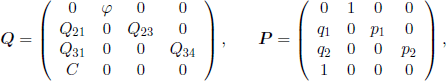
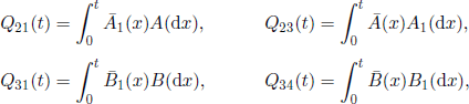
Matrices Q , P, and F are
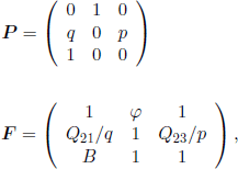
with
![]()
The stationary distribution is
![]()
Let v = (1, l, p) and m = (m1, m2, m3)′, with ![]() ,
, ![]() ,. Thus we obtain
,. Thus we obtain
![]()
The limit availability is
![]()
The mean times are:
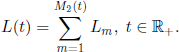
EXAMPLE 5.19.– (Successive delay system.) As a second example, we present a biological system with two successive delays. Let (F) be a biological factory and (U) a steam generation plant supplying the factory. If the unit fails for more than a critical time τ1 (delay 1), the biological substances die and a new repair is necessary (failure mode 1). In this case, if the failure lasts for a critical time τ2 (delay 2) after the first failure time τ1 , then essential parts of the biological factory are damaged (failure mode 2) and a long repair is necessary. In order to model such a system, let us consider the following states:
– state 1: F and U are working;
– state 2: U has failed for a time shorter than τ1 and F is working;
– state 3: U has failed for a time shorter than τ1 + τ2 but longer than τ1 and F has been stopped;
– state 4: U has failed for a time longer than τ1 + τ2 and F has been stopped.
Matrices Q and P are
with
where F is the d.f. of the lifetime of the steam generation plant, A is the d.f. of the repair time of the steam generation plant, B is the d.f. of the repair time of the factory (under failure mode 1), and C is the d.f. of the repair time of the factory (under failure mode 2); A1 and B1 are the d.f. of τ1 and τ2 , respectively. If τ1 and τ2 are fixed, then A1 and B2 are the Heaviside function 1(·); q1 and q2 are given by ![]() , and τ2 are random variables; if τ1 and τ2 are fixed, then q1= A(τ1), q2= B(τ2).
, and τ2 are random variables; if τ1 and τ2 are fixed, then q1= A(τ1), q2= B(τ2).
We have v = (1,1, p1, p2) and m = (m1, m2,m3, m4)′, with
Then, the stationary distribution is
![]()
The limit availability is
![]()
and the mean times are:
5.5. Reservoir models
Reservoir models comprise storage models with random inputs of resources in the stock. The goal is to optimize the demands (the outputs). The name of these models comes from the fact that they are used for water reservoirs (artificial lakes, dams). Let us consider a first example of a finite reservoir.
EXAMPLE 5.20.– Let X(n + 1) be the quantity of water which has flowed into the reservoir during the time interval (n, n + 1], n ∈ N. We assume that X(1), X(2), … are independent and have the same distribution. The reservoir has a finite capacity c, so the quantities of water that really enter the reservoir are
![]()
where Z(n) is the amount of water in the reservoir at time n ∈ ![]() and satisfies the general relationship [3.35]. The demands of water from the reservoir at times n = 1, 2, …, denoted by ξ1, ξ2, …, are supposed to be independent identically distributed r.v. Moreover, we suppose that the sequence (ξn, n ∈
and satisfies the general relationship [3.35]. The demands of water from the reservoir at times n = 1, 2, …, denoted by ξ1, ξ2, …, are supposed to be independent identically distributed r.v. Moreover, we suppose that the sequence (ξn, n ∈ ![]() +) is independent of the sequence
+) is independent of the sequence ![]() .
.
The amount of water that is really released from the reservoir at time n is given by
![]()
so relation [3.35] becomes
![]()
The first studies of this type of problem were proposed by P. Massé, H.E. Hurst, and P.A. Moran [HUR 51, HUR 55, MAS 46, MOR 59]; a study of the models developed until 1965 can be found in [PRA 65a].
For the use of semi-Markov models for this type of problem see [BAL 79, ÇIN71a, SEN 73, SEN 74b]; we will present in the following two such models.
5.5.1. Model I
Let Tn = T(n), n ∈ ![]() , denote the random instants when either an input or an output of water occurs. We assume that an input and an output cannot occur at the same time and that T0 = 0. Let Jn,n ∈
, denote the random instants when either an input or an output of water occurs. We assume that an input and an output cannot occur at the same time and that T0 = 0. Let Jn,n ∈ ![]() , be the r.v. taking either the value 1 if at instant Tn there is an input, or the value 2 if at instant Tn there is an output. The sequence ((Jn, Tn), n ∈
, be the r.v. taking either the value 1 if at instant Tn there is an input, or the value 2 if at instant Tn there is an output. The sequence ((Jn, Tn), n ∈ ![]() ) is a Markov renewal process with state space {1, 2} ×
) is a Markov renewal process with state space {1, 2} × ![]() .
.
Let An and Bn be the quantities of water that respectively enter the reservoir or are delivered from it at time Tn (obviously, An > 0⇔ Bn = 0); let us also denote by Z(t) the water amount in the reservoir at time t. Then, for Tn ≤ t ≤ Tn+1, we have
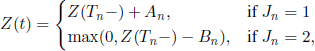
where ![]() .
.
The semi-Markov kernel of the Markov renewal process ((Jn, Tn), n ∈ ![]() ) is
) is
![]()
and let
![]()
We suppose that 0 < p, q < 1 and that the sequences of r.v. (An,n ∈ ![]() ) and (Bn, n ∈
) and (Bn, n ∈ ![]() ) are independent, each of them consisting in positive i.i.d. r.v., with α =
) are independent, each of them consisting in positive i.i.d. r.v., with α = ![]() (An) < ∞ and β =
(An) < ∞ and β = ![]() (Bn) < ∞.
(Bn) < ∞.
We are interested in obtaining results for the quantities of non-delivered water because of the too low levels of water stock in the reservoir. This kind of result is important for economical analyses prior to the construction of reservoirs.
We denote by tn(i), i = 1,2, the nth hitting time of state i by the process (Jn,n ∈ ![]() ), i.e. t0(i) = 0, t1(i) = min{m > 0 | Jm = i}, tn(i) = min{m > tn−1 |Jm = i}, n > 1. If we note Z(n) = Z(Tn−), n ∈
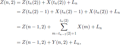
), i.e. t0(i) = 0, t1(i) = min{m > 0 | Jm = i}, tn(i) = min{m > tn−1 |Jm = i}, n > 1. If we note Z(n) = Z(Tn−), n ∈ ![]() +, (Z(l) = Z(0)), and Z{n, i) = Z{tn(i) + 1), i = 1,2, then Z(n, 1) is the amount of water in the reservoir just after the nth release and Z(n, 2) is the amount in the reservoir just after the nth demand. From [5.28] we obtain
+, (Z(l) = Z(0)), and Z{n, i) = Z{tn(i) + 1), i = 1,2, then Z(n, 1) is the amount of water in the reservoir just after the nth release and Z(n, 2) is the amount in the reservoir just after the nth demand. From [5.28] we obtain
where In(i) is the indicator function (i.e. the characteristic function) of the event (Jn = i).
If we set ![]() , relation [5.29] becomes
, relation [5.29] becomes
and the chain ((Jn,Xn),n ∈ ![]() ) is a J − X process with values in {1, 2} ×
) is a J − X process with values in {1, 2} × ![]() . If we assume that the chain (Jn, n ∈
. If we assume that the chain (Jn, n ∈ ![]() ) is ergodic, then a stationary (invariant) distribution π = (π1, π2) of (Jn, n ∈
) is ergodic, then a stationary (invariant) distribution π = (π1, π2) of (Jn, n ∈ ![]() ) exists, given by π =q(p + q)−1, π2 = p(p + q)−l, which is also stationary distribution for the chain ((Jn,Xn), n ∈
) exists, given by π =q(p + q)−1, π2 = p(p + q)−l, which is also stationary distribution for the chain ((Jn,Xn), n ∈ ![]() ). Thus we have
). Thus we have
![]()
Since
![]()
we get
![]()
Let us denote by ![]() , the stock variations between two successive passages through state i. As the r.v. (Y(n, i), n ≥ 2) arei.i.d. ([LIM 01], p. 90) and
, the stock variations between two successive passages through state i. As the r.v. (Y(n, i), n ≥ 2) arei.i.d. ([LIM 01], p. 90) and ![]() , we obtain
, we obtain
These relations give the mean variation value between two successive inputs into the reservoir and, respectively, between two successive outputs from the reservoir.
Setting ![]()
![]() , we have the following result.
, we have the following result.
THEOREM 5.21.– ([BAL79]) If qα − pβ < 0, then, for n → ∞, the r.v. Z(n, 1) and Z(n, 2) converge in distribution to ![]() , respectively to
, respectively to ![]() , for any initial value Z(0) of the stock level.
, for any initial value Z(0) of the stock level.
Note that both limits in Theorem 5.21 are finite. Indeed, ![]() a.s., (Y(n, i), n ≥ 2) is a sequence of i.i.d. r.v., and, from the law of large numbers we obtain
a.s., (Y(n, i), n ≥ 2) is a sequence of i.i.d. r.v., and, from the law of large numbers we obtain
as n → ∞.
Let us now denote by Ln the quantity non-delivered at the nth demand because of the too low level of the water stock at that time. Then
![]()
and, from [5.30], we obtain
which gives
where ![]() is the total quantity non-delivered during the first n demands.
is the total quantity non-delivered during the first n demands.
Let ![]() ; the following theorem focuses on the non-delivered quantity due to an insufficient stock level.
; the following theorem focuses on the non-delivered quantity due to an insufficient stock level.
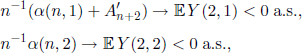
THEOREM 5.22.– ([BAL 79]) For n → ∞ we have:
(i) ![]() ;
;
(ii) If qα − pβ < 0 and α′, β′ ∞, then the r.v.
![]()
is asymptotically normal N(0, 1), where ![]() .
.
Proof.– (main steps) From [5.30] we obtain that
![]()
where ![]() . This result implies that [BAL 79, GRI 76, LIM 99]
. This result implies that [BAL 79, GRI 76, LIM 99]
![]()
so (i) is a consequence of [5.32].
To prove (ii), let us note that α(n, 2) is a sum of i.i.d. r.v. (except, possibly, the first one). Therefore, it satisfies the central limit theorem; moreover, from Theorem 5.21 we get that n−1/2 Z(n, 2) converges in probability to 0 and ![]() .
.
If we denote by L(t) the total quantity non-delivered during the interval [0, t] because of an insufficient stock and if we let
![]()
then
Let us introduce the following notation:
We can now state a result concerning the asymptotic behavior of the r.v. L(t).
THEOREM 5.23.– ([BAL 79]) If θ1,θ2< ∞, then, for t → ∞, we have:
(i) ![]() , a.s.;
, a.s.;
(ii) The. ![]() is asymptotically normal N(0,1), where
is asymptotically normal N(0,1), where
and
![]()
5.5.2. Model II
Let us denote by T0 = 0, T1, T2, … the successive random instants when an input occurs and by J0, J1, J2, … the corresponding amounts of these successive inputs. We assume that the sequence of r.v. (Jn, Tn, n ∈ ![]() ) is a regular Markov renewal process with values in
) is a regular Markov renewal process with values in ![]() ×
× ![]() and semi-Markov kernel Q(x, A, t), t, x ∈
and semi-Markov kernel Q(x, A, t), t, x ∈ ![]() , A ∈ β
(see subsection 5.2.1 or [LIM 01], pp. 31-33, 95). Let the r.v. Y0: Ω →
, A ∈ β
(see subsection 5.2.1 or [LIM 01], pp. 31-33, 95). Let the r.v. Y0: Ω → ![]() denote the initial stock level. If this initial value is x, then the output rate (intensity) is r(x), where r:
denote the initial stock level. If this initial value is x, then the output rate (intensity) is r(x), where r: ![]() →
→ ![]() is an increasing continuous function with r(0) = 0. We also introduce the r.v. Z(t) for the total quantity of water which has flowed into the reservoir during the period [0, t], i.e.
is an increasing continuous function with r(0) = 0. We also introduce the r.v. Z(t) for the total quantity of water which has flowed into the reservoir during the period [0, t], i.e. ![]() . If Y(t) is the amount of water existing in the reservoir at time t, then Y(t) satisfies the functional relationship
. If Y(t) is the amount of water existing in the reservoir at time t, then Y(t) satisfies the functional relationship
The process ![]() is an
is an ![]() -valued stochastic process that will be specified in the following. First of all, we give the following lemma whose proof, based on the continuity of the function r, is straightforward.
-valued stochastic process that will be specified in the following. First of all, we give the following lemma whose proof, based on the continuity of the function r, is straightforward.
LEMMA 5.24.– ([ÇIN 71a]) Equation
has a unique measurable solution q and the functions q(· , t) and q(x, ·) are increasing and continuous.
As the function ![]() is constant on intervals [Tn, Tn+1), this implies that the function
is constant on intervals [Tn, Tn+1), this implies that the function ![]() satisfies the differential equation y′ = −r(y) with the initial condition y(0) = Y(Tn). Therefore,
satisfies the differential equation y′ = −r(y) with the initial condition y(0) = Y(Tn). Therefore,
![]()
where q is the solution of equation [5.34]. From the continuity of q(x, · ) we obtain that Y (t) has a left limit at Tn+1 and the jump at this point is Jn+1, which is also the jump of Z(t) at the same point.
Taking into account all this discussion we can state the following result.
THEOREM 5.25.– ([ÇIN 71a]) For n ∈ ![]() , let us define Y (n) by the recurrence relations
, let us define Y (n) by the recurrence relations
![]()
Then Y(t) defined by the relations Y(t) = q(Y(n)+ Jn, t − Tn)for Tn ≤ t < ![]() , is the unique solution of equation [5.33].
, is the unique solution of equation [5.33].
For the r.v. ![]() , with values in
, with values in ![]() , we have the following result.
, we have the following result.
THEOREM 5.26.– The sequence ![]() is a Markov renewal process, with values in
is a Markov renewal process, with values in ![]() and semi-Markov kernel
and semi-Markov kernel
![]()
where ![]() is the indicator function of set B.
is the indicator function of set B.
Proof.– We do not investigate here if ![]() and Wn are measurable, we only derive the expression of the function
and Wn are measurable, we only derive the expression of the function ![]() . We have
. We have
COROLLARY 5.27.– The sequence of r.v. (Wn, n ∈ ![]() ) is a Markov chain with transition function
) is a Markov chain with transition function
![]()
Let us note that the sequence of r.v. (Y (n), n ∈ ![]() ) is not a Markov chain in the general case; however, if Jn+1 is independent of Jn and of the time Tn+1 −Tn between two successive inputs, then ((Y (n), Tn), n ∈
) is not a Markov chain in the general case; however, if Jn+1 is independent of Jn and of the time Tn+1 −Tn between two successive inputs, then ((Y (n), Tn), n ∈ ![]() ) is a Markov renewal process. More precisely, we have the following result.
) is a Markov renewal process. More precisely, we have the following result.
THEOREM 5.28.– Let us suppose that the semi-Markov kernel of the Markov renewal process ((Jn, Tn), n ∈ ![]() ) satisfies the condition
) satisfies the condition
where γ is a probability on β+. If G(·, ·) is such that
(i) G(x, ·)is a distribution function that is zero on (−∞, 0);
(ii) G(·, t) is β+-measurable,
then the chain ((Y(n),Tn),n ∈ ![]() ) is a Markov renewal process with the semi-Markov kernel
) is a Markov renewal process with the semi-Markov kernel
![]()
PROOF.– As ((Jn, Tn), n ∈ ![]() ) is a Markov renewal process, condition [5.35] is equivalent to
) is a Markov renewal process, condition [5.35] is equivalent to
![]()
Thus, for ![]() we have
we have
Using this result and the definition of (Y(n),n ∈ ![]() ) we obtain
) we obtain
We want to compute the transition function of the process (Y(t),t ∈ ![]() ); more precisely, let
); more precisely, let ![]() xy(·) be the conditional probability
xy(·) be the conditional probability ![]()
![]() . For any measurable function
. For any measurable function ![]() we define the operator
we define the operator
![]()
which is a contraction in the normed vector space ![]() f bounded Borel function} with the norm
f bounded Borel function} with the norm ![]() .
.
From Theorem 5.25 we obtain that for any ![]() we have
we have
and, if Qn is the nth iterate of Q, then
The following theorem specifies how the probability ![]() can be computed.
can be computed.
THEOREM 5.29.– For fixed A ∈ β, let
![]()
Then ![]() and it satisfies the equation
and it satisfies the equation
where
Equation [5.38] has a unique solution given by
Proof.– We omit here the details on the measurability of f.
If T1 > t, then Y (t) = q(J0 + Y0, t) and, for A ∈ β, we have
![]()
on the set (T1 > t). On the other hand, Theorems 5.25 and 5.26 yield
![]()
So, from [5.36] and [5.39] we get
If we denote by 1 the constant unit function on ![]() , then
, then
![]()
and therefore 0 ≤ g ≤ 1 −Q1. Consequently,
![]()
for any m ∈ ![]() . Thus
. Thus ![]() and the convergence of the series
and the convergence of the series ![]() is proved.
is proved.
From [5.38], we obtain by induction on n that
and, as 0 ≤ f ≤ 1, we get 0 ≤ Qn f ≤ Q1. On the other side, from [5.37] we get ![]() , because the process is regular; therefore,
, because the process is regular; therefore, ![]() in [5.41], then we obtain [5.40].
in [5.41], then we obtain [5.40].
Let us now consider the moment when the reservoir runs dry for the first time, denoted by S = inf{t | Y(t) = 0}, with the convention S = ∞ if Y(t) > 0 for all t ∈ ![]() . As Y(·) is right continuous, we will have Y(S) = 0 if and only if S < ∞. If we let b = sup{x | r(x) = 0}, then from b > 0 we would obtain S = ∞ for Y0 + j0 > 0; so we can suppose that 6 = 0, i.e. r(x) > 0 for all x > 0. Additionally, if Y0> 0, then S = ∞ except for the case when there exists a δ > 0 such that
. As Y(·) is right continuous, we will have Y(S) = 0 if and only if S < ∞. If we let b = sup{x | r(x) = 0}, then from b > 0 we would obtain S = ∞ for Y0 + j0 > 0; so we can suppose that 6 = 0, i.e. r(x) > 0 for all x > 0. Additionally, if Y0> 0, then S = ∞ except for the case when there exists a δ > 0 such that ![]() . To avoid this situation, we have to assume that
. To avoid this situation, we have to assume that ![]() .
.
For any x ∈ ![]() , let us denote by τ(x) the necessary time for the reservoir to run dry if no input occurs, τ(x) = inf{t > 0 | q(x, t) = 0}. We note that τ is finite, continuous, strictly increasing, and τ(0) = 0; moreover, τ(x) =
, let us denote by τ(x) the necessary time for the reservoir to run dry if no input occurs, τ(x) = inf{t > 0 | q(x, t) = 0}. We note that τ is finite, continuous, strictly increasing, and τ(0) = 0; moreover, τ(x) = ![]() .
.
Results on the distribution of the r.v. S and on the asymptotic behavior of Y(t) can be found in [ÇIN 71a].
5.6. Queues
Queueing theory is concerned with models for various items or demands, waiting to be served in a certain order. These demands can be: phone calls, customers waiting to be served at a checkout counter, cars at crossroads, airplanes asking for landing permission, etc. The mathematical problems linked to all these examples are basically the same.
Queueing theory is attractive because it can be easily described by means of its intuitive characteristics. In general, queueing systems are non-Markovian, non-stationary, and difficult to study. In any queueing analysis there are several common elements that we will describe in the following. The demands (customers) arrive to the servers (service points), where there could also be other clients. It is possible that a customer needs to wait for a server to become available (free). When there is an available server, the customer is served and then he leaves the system.
Let us first give some more details on queueing systems, before presenting some adapted models. For example, the points that need to be specified are:
(a)How do the customers arrive in the system? Here are some cases:
– the arrival process is a Poisson process (denoted by M);
– the successive interarrival times have a known constant value (denoted by D);
– the successive interarrival times have a general probability distribution (denoted by G).
(b)How long is the service time of a customer? Here we can have:
– the service time has an exponential distribution (denoted by M);
– the service time has a known constant value (denoted by D);
– the service time has a general probability distribution (denoted by G).
(c)The number of servers in the system is generally denoted by s, with 1 ≤ s ≤ ∞.
Using this notation (introduced by D. G. Kendall), for an M(λ)/G(μ)/s queue, the arrivals are Poissonian of parameter A, the service time has a general distribution of mean μ, and there are s servers in the system.
There are many works on classic queueing models, like [KAR 75, PRA 80, RES 92, TAK 62]. For the use of semi-Markov processes in this type of model, see [ASM 87, BAR 82, BOE 81, ÇIN 67b, ÇIN 67a, NEU 66, SIL 80].
5.6.1. The G/M/1queue
We assume that the demands arrive at random times, each interarrival time has a probability distribution G, and the service time is exponentially distributed with parameter λ.
Let T1, T2, … be the arrival times of the demands and Jn be the number of units in the system at instant Tn − 0, i.e. just before the nth arrival. As Jn+1 depends only on Jn and Xn+1 = Tn+1 − Tn, and Xn+1 is independent of J0, J1, …, Jn, X1, …, Xn, we obtain that ((Jn, Tn), n ∈ ![]() ) is a Markov renewal process. In this case, Qij(t) =
) is a Markov renewal process. In this case, Qij(t) = ![]() Jn+1 = j, Xn+1≤ t | Jn = i) depends on i and j, but
Jn+1 = j, Xn+1≤ t | Jn = i) depends on i and j, but ![]() (Xn+1 ≤ t | Jn = i) = G(t) does not depend on i.2 If we let
(Xn+1 ≤ t | Jn = i) = G(t) does not depend on i.2 If we let ![]() , then we can prove that the chain (Jn, n ∈
, then we can prove that the chain (Jn, n ∈ ![]() ) is non-recurrent or recurrent, depending on Am < 1 or λm ≥ 1. In the case when λm ≥ 1, there is a unique stationary measure α = (α0, α1, …), α0= 1, given by
) is non-recurrent or recurrent, depending on Am < 1 or λm ≥ 1. In the case when λm ≥ 1, there is a unique stationary measure α = (α0, α1, …), α0= 1, given by ![]() , where β is a solution of equation
, where β is a solution of equation ![]() , and
, and ![]() is the Laplace transform of G(t)3; moreover, β < 1 if and only if λm ≥ 1 [KAR 75, TAK 62].
is the Laplace transform of G(t)3; moreover, β < 1 if and only if λm ≥ 1 [KAR 75, TAK 62].
Let Z(t) be the number of units in the system at time t (units waiting to be served or being served). If we introduce the notation
for any j ∈ ![]() , then conditioning on X1 we obtain the Markov renewal equation
, then conditioning on X1 we obtain the Markov renewal equation
where ![]() . This equation has a unique solution given by [ÇIN 69b]
. This equation has a unique solution given by [ÇIN 69b]
![]()
The following result concerns the asymptotic behavior of ![]() (Y(t) = k), as t tends to infinity.
(Y(t) = k), as t tends to infinity.
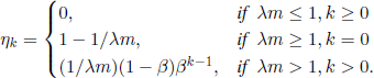
THEOREM 5.30.– ([ÇIN71a]) For all k ∈ ![]() , the limit ηk = limt→∞
, the limit ηk = limt→∞ ![]() (Y(t) = k) exists and is independent of j. More exactly, we have
(Y(t) = k) exists and is independent of j. More exactly, we have
5.6.2. The M/G/1queue
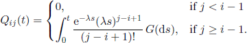
Let T0 = 0, T1, T2,… be the departure moments of the units from the system and Jn be the number of units in the system at instant Tn + 0, i.e. just after the instant Tn. The arrivals form a Poisson process of parameter A and the service time has a distribution G. The sequence ((Jn, Tn), n ∈ ![]() ) is a Markov renewal process, whose semi-Markov kernel is given by [SIL 80]
) is a Markov renewal process, whose semi-Markov kernel is given by [SIL 80]
Let ![]() ; as opposed to the previous model, the states of (Jn, n ∈
; as opposed to the previous model, the states of (Jn, n ∈ ![]() ) are recurrent or non recurrent depending on λm ≤ 1 or λm > 1. In the case λm ≤ 1, the chain has a stationary measure β = (β0, β1, …), whose generating function is
) are recurrent or non recurrent depending on λm ≤ 1 or λm > 1. In the case λm ≤ 1, the chain has a stationary measure β = (β0, β1, …), whose generating function is
If λm = 1, then this stationary measure is σ-finite [KAR 75].
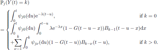
Let Y(t) be the number of units in the system at time t ∈ ![]() . If Y(t) = k and just after the time TN(t) there are v units in the system, then during the interval TN(t), t] there are k − v arrivals. Therefore, if we let
. If Y(t) = k and just after the time TN(t) there are v units in the system, then during the interval TN(t), t] there are k − v arrivals. Therefore, if we let
![]()
we can prove that
The following result concerns the asymptotic behavior of ![]() j(Y(t) = k), as t tends to infinity.
j(Y(t) = k), as t tends to infinity.
THEOREM 5.31.– ([ÇIN71a]) For any k ∈ ![]() , the limit ηk = lim→∞
, the limit ηk = lim→∞ ![]() (Y(t) = k) exists and is independent of j. If λm ≥ 1, then ηk = 0, k ∈
(Y(t) = k) exists and is independent of j. If λm ≥ 1, then ηk = 0, k ∈ ![]() ; if λm < 1, then ηk = βk, k ∈
; if λm < 1, then ηk = βk, k ∈ ![]() , from [5.43].
, from [5.43].
Remark. There is an interesting relation between the busy period in the M/G/1 model and the total number of objects up to extinction in the B-G-W model (see Section 6.1). Further details could be found in [NEU 69].
5.7. Digital communication channels
In order to evaluate the performance of error-detecting and error-correcting codes, we use digital channel models, models that describe the statistical characteristics of the error sequences. A standard problem in such a context is to evaluate the probability that a block of n symbols contains m errors (m ≤ n).
The real channels can have different levels of statistical dependence of errors. These errors can appear from various reasons, like impulse perturbations, random interruptions in the functioning of equipments, crosstalk noise affecting the reliability of symbol transmission, etc.
When representing a channel by a model, we can use simulations to analyze the performance of different control techniques.
For finite state space Markov models see [DUM 79, GIL 60, FRI 67], while renewal models can be found in [ADO 72, ELL 65]. Semi-Markov models are more general and we will give below an example of this type [DUM 83].
First of all, let us present some characteristics of discrete-time semi-Markov models. For a discrete-time semi-Markov process with state space E = {1, …, s}, the matrix-valued function (Qij(t), i, j ∈ E), t ∈ ![]() , is replaced by the matrix-valued function (cij (t), i, j ∈ E), t ∈
, is replaced by the matrix-valued function (cij (t), i, j ∈ E), t ∈ ![]() , defined by
, defined by
![]()
For the chain ![]() with values in E ×
with values in E × ![]() , relation [5.1] becomes
, relation [5.1] becomes
Note that the Markov renewal equation associated with Pij(t) = ![]() (Z(t) = j | Z0 = i), t ∈
(Z(t) = j | Z0 = i), t ∈ ![]() , is
, is
If we note
![]()
then
![]()
We consider a binary symmetric additive communication channel. The state space E is partitioned into two subsets A and B. We suppose that the evolution of the channel is described by a semi-Markov process (Z(t), t ∈ ![]() ). The transitions occur at times Tn, n = 1, 2, …, which represent the beginning of a bit sent through the channel. The error process (e(t), t ∈
). The transitions occur at times Tn, n = 1, 2, …, which represent the beginning of a bit sent through the channel. The error process (e(t), t ∈ ![]() ), with values in {0,1}, is obtained from
), with values in {0,1}, is obtained from ![]() . Put into words, this means that the states of A do not generate errors, whereas when the source of the noise is in one of the states of B, then errors surely occur. An interval without errors is a sequence of zeros between two errors. The length of an interval without errors is defined as being equal to 1+ the number of zeros between two errors. Let
. Put into words, this means that the states of A do not generate errors, whereas when the source of the noise is in one of the states of B, then errors surely occur. An interval without errors is a sequence of zeros between two errors. The length of an interval without errors is defined as being equal to 1+ the number of zeros between two errors. Let
![]()
be the probability to correctly receive at least m bits after having received one error and let also
![]()
be the probability to receive at least m errors after having correctly received one bit.
We will calculate the probabilities P(0m/1) and P(lm/0). We have
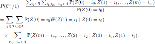
On the one hand, as i0 ≠ i1 for i0 ∈ A and i1 ∈ B, we infer that the events (Z(0) = i0, Z(1) = i1) and (J0 = i0, J1= i1) have the same probability and we can write
On the other hand, if we note
![]()
then, in the same way as we did for obtaining [5.45], we find
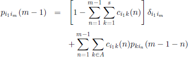
and [5.46] can be written as
where α = (α1, …, αs) is the distribution of the r.v. J0 (the initial distribution of the process).
The probabilities Pi1im (m − 1), m = 2, 3, …, can be obtained from the recurrence relations [5.47]; afterward, the probability P(0m/1) is obtained from [5.48]. Similarly, we can obtain the probability P(lm/0).
These probabilities are computed in [FRI 67] for a Markovian evolution of the channel.
In [ADO 72], the function
![]()
was introduced in order to characterize digital channels. For Markov models, the function α has an exponential asymptotic behavior, assumption that is not satisfied for all channels in real applications.
1. We use the convention that subscript 0 denotes the partition corresponding to the set U, whereas subscript 1 denotes the partition corresponding to the set D. For instance, α0 is the restriction of α to U.
2.Generally,![]() depends on i.
depends on i.
3. Thatis, ![]() .
.