
9.4 The Gibbs sampler
9.4.1 Chained data augmentation
We will now restrict our attention to cases where m=1 and the augmented data ![]() consists of the original data
consists of the original data ![]() augmented by a single scalar z (as in the linkage example). The algorithm can then be expressed as follows: Start from a value
augmented by a single scalar z (as in the linkage example). The algorithm can then be expressed as follows: Start from a value ![]() generated from the prior distribution for η and then iterate as follows:
generated from the prior distribution for η and then iterate as follows:
(There is, of course, a symmetry between η and z and the notation is used simply because it arose in connection with the first example we considered in connection with the data augmentation algorithm.) This version of the algorithm can be referred to as chained data augmentation, since it is easy to see that the distribution of the next pair of values ![]() given the values up to now depends only on the present pair and so these pairs move as a Markov chain. It is a particular case of a numerical method we shall refer to as the Gibbs sampler. As a result of the properties of Markov chains, after a reasonably large number T iterations the resulting values of η and z have a joint density which is close to
given the values up to now depends only on the present pair and so these pairs move as a Markov chain. It is a particular case of a numerical method we shall refer to as the Gibbs sampler. As a result of the properties of Markov chains, after a reasonably large number T iterations the resulting values of η and z have a joint density which is close to ![]() , irrespective of how the chain started.
, irrespective of how the chain started.
Successive observations of the pair ![]() will not, in general, be independent, so in order to obtain a set of observations which are, to all intents and purposes, independently identically distributed (i.i.d.), we can run the aforementioned process through T successive iterations, retaining only the final value obtained, on k different replications.
will not, in general, be independent, so in order to obtain a set of observations which are, to all intents and purposes, independently identically distributed (i.i.d.), we can run the aforementioned process through T successive iterations, retaining only the final value obtained, on k different replications.
We shall illustrate the procedure by the following example due to Casella and George (1992). We suppose that π and y have the following joint distribution:
![]()
and that we are interested in the marginal distribution of y. Rather than integrating with respect to π (as we did at the end of Section 3.1), which would show that y has a beta-binomial distribution, we proceed to find the required distribution from the two conditional distributions:
![]()
This is a simple case in which there is no observed data ![]() . We need to initialize the process somewhere, and so we may as well begin with a value of π which is chosen from a U(0, 1) distribution. Again the procedure is probably best expressed as an
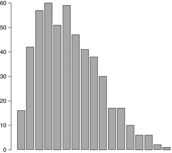
. We need to initialize the process somewhere, and so we may as well begin with a value of π which is chosen from a U(0, 1) distribution. Again the procedure is probably best expressed as an ![]() program, which in this case constructs a histogram as well as the better and smoother estimate resulting from taking the ‘current’ distribution at the end of each iteration:
program, which in this case constructs a histogram as well as the better and smoother estimate resulting from taking the ‘current’ distribution at the end of each iteration:
nr < - 50
m < - 500
k < - 10
n < - 16
alpha < - 2.0
beta < - 4.0
lambda < - 16.0
maxn < - 24
h < - rep(0,n+1)
for (i in 1:m)
{
pi < - runif(1)
for (j in 1:k)
{
y < - rbinom(1,n,pi)
newalpha < - y + alpha
newbeta < - n - y + beta
pi < - rbeta(1,newalpha,newbeta)
}
for (t in 0:n)
{
if (t == y)
h[t+1] < - h[t+1] + 1
}
}
barplot(h)
The resultant histogram is given as Figure 9.2. References for the generation of ‘pseudo-random’ numbers can be found in the previous section. An implementation in ![]() with T=10 iterations replicated m=500 times for the case n=16,
with T=10 iterations replicated m=500 times for the case n=16, ![]() and
and ![]() will, as Casella and George remark, give a very good approximation to the beta-binomial density.
will, as Casella and George remark, give a very good approximation to the beta-binomial density.
Figure 9.2 Barplot of values of y between 0 and 16.
9.4.2 An example with observed data
Gaver and O’Muircheartaigh (1987) quote the data later on the rates of loss of feedwater flow for a collection of nuclear power systems. In the following table, a small set of data representing failure of pumps in several systems of the nuclear plant Farley 1 is given. The apparent variation in failure rates has several sources.
Number yi of pump failures in ti thousand hours

It should seem plausible that the number of failures in any fixed time interval should have a Poisson distribution and that the mean of this distribution should be proportional to the length of the interval, with a constant of proportionality varying from pump to pump. It seems sensible to assume that these constants come from the conjugate family, the multiples of chi-squared (cf. Section 3.4), so that
![]()
For the moment, we shall regard it as known that ![]() . We seek the marginal distributions
. We seek the marginal distributions ![]() , but unfortunately these do not have a closed form. We need to write
, but unfortunately these do not have a closed form. We need to write
![]()
Now
![]()
from which it easily follows that

It is then clear from Appendix A.2 that
![]()
where
![]()
As for S0, we find that if we take a ![]() prior for S0, then
prior for S0, then
This is clearly a chi-squared distribution, so that
![]()
with
![]()
In accordance with the general principal of the Gibbs sampler, we now take a value of S0 and then generate values of the ![]() , then use those values to generate a value of S0, then use this new value to generate new values of the
, then use those values to generate a value of S0, then use this new value to generate new values of the ![]() , and so on.
, and so on.
An ![]() program to carry out this process is as follows:
program to carry out this process is as follows:
N < - 10000
burnin < - 1000
k < - 10
y < - c(5,1,5,14,3,19,1,1,4,22)
t < - c(94.320,15.720,62.880,125.760,5.240,
31.440,1.048,1.048,2.096,10.480)
r < - y/t
U < - 1.0
rho < - 0.2
nu < - 1.4
S < - rep(NA,N)
S[1] < - 2.0
theta < - matrix(NA,nrow=N,ncol=k)
theta[1,] < - rep(1.0,k)
for (j in 2:N) (
for (i in 1:k) {
theta[j,i] < - (S[j-1]+2*t[i])^ (-1)*rchisq(1,nu+2*y[i])
}
S[j] < - (U+sum(theta[j,]))^ (-1)*rchisq(1,rho+k*nu)
}
Strunc < - S[burnin:N]
thetatrunc < - theta[burnin:N,]
thetamean < - apply(thetatrunc,2,mean)
thetasd < - apply(thetatrunc,2,sd)
thetastats < - cbind(thetamean,thetasd)
colnames(thetastats) < - c(“mean”,“sd”)
cat(“
Pump means estimated as
”)
print(thetastats)
cat(“
S has mean”,mean(Strunc),
       “and s.d.”,sd(Strunc),“
”)
The results of a run of N=10 000 (of which the first 1000 are ignored) are as follows:
| System (i) | Mean | s.d. |
| 1 | 0.05989735 | 0.02507362 |
| 2 | 0.10256774 | 0.07870071 |
| 3 | 0.08914099 | 0.03705638 |
| 4 | 0.11561089 | 0.03005465 |
| 5 | 0.60907691 | 0.31762446 |
| 6 | 0.60667401 | 0.13747133 |
| 7 | 0.89859718 | 0.72278527 |
| 8 | 0.89560013 | 0.71677873 |
| 9 | 1.58454532 | 0.75715648 |
| 10 | 1.99107727 | 0.42022407 |
It turns out that S0 has mean 1.849713 and s.d. 0.7906609, but this is less important.
9.4.3 More on the semi-conjugate prior with a normal likelihood
Recall that we said in Section 9.2 that in the case where we have observations x1, x2, … , ![]() , we say that we have a semi-conjugate or conditionally conjugate prior for θ and
, we say that we have a semi-conjugate or conditionally conjugate prior for θ and ![]() (which are both supposed unknown) if
(which are both supposed unknown) if
![]()
independently of one another.
Conditional conjugacy allows the use of the procedure described in Section 9.3, since conditional on knowledge of ![]() we know that the posterior of θ is
we know that the posterior of θ is
![]()
where
![]()
(cf. Section 2.3). Then, conditional on knowledge of θ we know that the posterior of ![]() is
is
![]()
where
![]()
(cf. Section 2.7).
To illustrate this case, we return to the data on wheat yield considered in the example towards the end of Section 2.13 in which n=12, ![]() and S=13 045 which we also considered in connection with the EM algorithm. We will take the same prior we used in connection with the EM algorithm, so that we will take
and S=13 045 which we also considered in connection with the EM algorithm. We will take the same prior we used in connection with the EM algorithm, so that we will take ![]() with S0=2700 and
with S0=2700 and ![]() and (independently of
and (independently of ![]() )
) ![]() where
where ![]() and
and ![]() .
.
We can express an ![]() program as a procedure for finding estimates of the mean and variance of the posterior distributions of θ from the values of θ generated. It is easy to modify this to find other information about the posterior distribution of θ or of
program as a procedure for finding estimates of the mean and variance of the posterior distributions of θ from the values of θ generated. It is easy to modify this to find other information about the posterior distribution of θ or of ![]() .
.
iter < - 10 # Number of iterations of the EM algorithm
m < - 500 # Number of replications
t < - 10 # Number of iterations
n < - 12
xbar < - 119
sxx < - 13045
s0 < - 2700
nu0 < - 11
n0 < - 15
theta0 < - 110
phi0 < - s0/(n0*(nu0-2))
thetabar < - 0
phibar < - 0
phi < - sxx/(n-1) # Initialize
thetafinal < - rep(0,m)
phifinal < - rep(0,m)
for (j in 1:m) # Replicate m times
{
for (s in 1:t) # Iterate t times
{
phi1 < - 1/((1/phi0)+(n/phi))
theta1 < - phi1*((theta0/phi0)+(n*xbar/phi))
![]()
theta < - theta1+sqrt(phi1)*rnorm(1)
# S1 = S0 + Σ(x (i) - θ)2
s1 < - s0+sxx+n*(xbar-theta)*(xbar-theta)
![]()
phi < - s1/rchisq(1,nu0+n)
}
thetafinal[j] < - theta
phifinal[j] < - phi
}
thetabar < - mean(thetafinal)
thetavar < - var(thetafinal)
cat(“Posterior for theta has mean”,thetabar,
    “and variance”,thetavar,“
”)
This procedure can be implemented using algorithms in Kennedy and Gentle (1980); an implementation in ![]() with k=500 replications of T=10 iterations resulted in
with k=500 replications of T=10 iterations resulted in ![]() and
and ![]() so that the standard deviation is 3.789. (Note that there is no reason to think that the posterior of θ is symmetrical in this case, so the mean as found here need not be exactly the same as the median which we found by the EM algorithm.) If we are prepared to modify the prior very slightly, so that
so that the standard deviation is 3.789. (Note that there is no reason to think that the posterior of θ is symmetrical in this case, so the mean as found here need not be exactly the same as the median which we found by the EM algorithm.) If we are prepared to modify the prior very slightly, so that ![]() is even, it can be implemented very easily with algorithms in Press et al. (1986–1993).
is even, it can be implemented very easily with algorithms in Press et al. (1986–1993).
Extensions of this methodology to deal with the general linear model are described by O’Hagan (1994, Sections 9.45 et seq.).
9.4.4 The Gibbs sampler as an extension of chained data augmentation
With the chained data augmentation algorithm, we had two stages in which we estimated alternately two parameters η and z. The Gibbs sampler can be regarded as a multivariate extension of the chained data augmentation algorithm in which we estimate r parameters ![]() ,
, ![]() , … ,
, … , ![]() . To use it, we take a starting point
. To use it, we take a starting point ![]() and then iterate as follows:
and then iterate as follows:
Then values of ![]() move as a Markov chain, so that once they get to a particular position, in thinking of where to go next they have no memory of where they have previously been. As we remarked earlier, in many cases this will mean that values taken after a large number of iterations should have a distribution which does not depend on their starting distribution. There are complicated questions relating to the circumstances in which convergence to an equilibrium distribution occurs and, assuming that it does, the speed at which equilibrium is approached, which we will return to later.
move as a Markov chain, so that once they get to a particular position, in thinking of where to go next they have no memory of where they have previously been. As we remarked earlier, in many cases this will mean that values taken after a large number of iterations should have a distribution which does not depend on their starting distribution. There are complicated questions relating to the circumstances in which convergence to an equilibrium distribution occurs and, assuming that it does, the speed at which equilibrium is approached, which we will return to later.
The Gibbs sampler became widely known from the work of Geman and Geman (1984), although its roots can be traced back to Metropolis et al. (1953) and its use in this context was proposed by Turchin (1971). Its name arises from connections with the Gibbs distribution in statistical mechanics which are explained in Geman and Geman (op. cit.) or Ó Ruanaidh and Fitzgerald (1996, Chapter 4).
9.4.5 An application to change-point analysis
It is difficult to appreciate the Gibbs sampler without following through a realistic example in detail, but many real uses of the method involve distributions not dealt with in this book as well as other complications. We shall now consider in detail the case of a Poisson process with a change point which was first introduced in Section 8.1 on ‘The idea of a hierarchical model’. There are no undue complications in this example, although it necessarily takes a certain amount of work to deal with a problem involving so many parameters.
Recall that we supposed that ![]() for
for ![]() while
while ![]() for
for ![]() and that we took independent priors for the parameters
and that we took independent priors for the parameters ![]() such that
such that
Finally, we supposed that the hyperparameters γ and δ had prior distributions which were (independently of one another) multiples of chi-squared. In what follows, we shall take ![]() and
and ![]() . These priors are improper and it would be better to take
. These priors are improper and it would be better to take ![]() and
and ![]() as other authors have done. On the other hand, our choice enables us to restrict attention to gamma distributions with integer parameters and many computer systems make it easier to generate values from such distributions.
as other authors have done. On the other hand, our choice enables us to restrict attention to gamma distributions with integer parameters and many computer systems make it easier to generate values from such distributions.
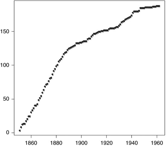
The actual data on the numbers of coal-mining disasters in the n=112 years from 1851 to 1962 inclusive were as follows:
The plot of the cumulative number of disasters against time given as Figure 9.3 appears to fall into two approximately straight sections, suggesting that disasters occurred at a roughly constant rate until a ‘change-point’ k when the average rate suddenly decreased. It, therefore, seems reasonable to try to fit the aforementioned model. If we are interested in the distribution of k, it rapidly appears that direct integration of the joint distribution presents a formidable task.
Figure 9.3 Cumulative number of disasters.
We can, however, proceed to find the conditional distribution of each of the parameters λ, μ and k and the hyperparameters γ and δ given all of the others and the data ![]() . For this purpose, we shall find it helpful to write
. For this purpose, we shall find it helpful to write
![]()
From the facts that we have a prior ![]() and data
and data ![]() for i=1, 2, … , k, it follows as in Section 3.4 on ‘The Poisson distribution’ that
for i=1, 2, … , k, it follows as in Section 3.4 on ‘The Poisson distribution’ that
![]()
where
![]()
or equivalently
![]()
has a two-parameter gamma distribution (see Appendix A). Similarly,
![]()
where
![]()
or equivalently
![]()
Next, we note that we have a prior ![]() and (since
and (since ![]() ) a likelihood for γ given λ of
) a likelihood for γ given λ of ![]() . It follows just as in Section 2.7 on ‘Normal variance’ that the posterior is
. It follows just as in Section 2.7 on ‘Normal variance’ that the posterior is
![]()
which we can express as
![]()
or equivalently
![]()
Similarly,
![]()
or equivalently
![]()
The distribution of k is not from any well-known parametric family. However, we can easily see that
![]()
so that (after dividing by ![]() ) we can write the log-likelihood as
) we can write the log-likelihood as
![]()
Since, the prior for k is UD(1, n), it follows that
![]()
Once we have these conditional distributions, we can proceed using the Gibbs sampler. The starting point of each iteration is not of great importance in this case, so we use plausible guesses of ![]() ,
, ![]() and k an integer somewhere near the middle of the range (it might seem better to pick k randomly between 1 and n, but there are computational difficulties about this approach and in any case we expect from inspection of the data that k is somewhere in the middle). A further indication of how to proceed is given in the
and k an integer somewhere near the middle of the range (it might seem better to pick k randomly between 1 and n, but there are computational difficulties about this approach and in any case we expect from inspection of the data that k is somewhere in the middle). A further indication of how to proceed is given in the ![]() program later, which uses only uniformly distributed random variates and one parameter gamma variates with integer parameters; the resulting analysis is slightly different from that in Carlin et al. (1992), but our restriction to integer parameters for the gamma variates makes the computation slightly simpler. We approximate the posterior density of k by Pr(k) which is found as the average over m replications of the current distribution p(k) for k after T iterations. We also find the mean of this posterior distribution.
program later, which uses only uniformly distributed random variates and one parameter gamma variates with integer parameters; the resulting analysis is slightly different from that in Carlin et al. (1992), but our restriction to integer parameters for the gamma variates makes the computation slightly simpler. We approximate the posterior density of k by Pr(k) which is found as the average over m replications of the current distribution p(k) for k after T iterations. We also find the mean of this posterior distribution.

A run in ![]() with m=100 replicates of t=15 iterations resulted in a posterior mean for k of 1889.6947, that is, 11 September 1889. A slightly different answer results from the use of slightly more realistic priors and the use of gamma variates with non-integer parameters. It is possible that the change is associated with a tightening of safety regulations as a result of the Coal Mines Regulation Act (50 & 51 Vict. c. 58 [1887]) which came into force on 1 January 1888.
with m=100 replicates of t=15 iterations resulted in a posterior mean for k of 1889.6947, that is, 11 September 1889. A slightly different answer results from the use of slightly more realistic priors and the use of gamma variates with non-integer parameters. It is possible that the change is associated with a tightening of safety regulations as a result of the Coal Mines Regulation Act (50 & 51 Vict. c. 58 [1887]) which came into force on 1 January 1888.
9.4.6 Other uses of the Gibbs sampler
The Gibbs sampler can be used in a remarkable number of cases, particularly in connection with hierarchical models, a small subset of which are indicated later. Further examples can be found in Bernardo et al. (1992 and 1996), Tanner (1996), Gatsonis et al. (1993 and 1995), Gelman et al. (2004), Carlin and Louis (2000) and Gilks et al. (1996).
9.4.6.1 Radiocarbon dating
Buck et al. (1996, Sections 1.1.1, 7.5.3 and 8.6.2) describe an interesting application to archaeological dating. Suppose that the dates of organic material from three different samples s are measured as x1, x2 and x3 and it is believed that, to a reasonable approximation, ![]() where
where ![]() is the age of the sample and
is the age of the sample and ![]() can be regarded as known. It can be taken as known that the ages are positive and less than some large constant k, and the time order of the three samples it is also regarded as known on archaeological grounds, so that
can be regarded as known. It can be taken as known that the ages are positive and less than some large constant k, and the time order of the three samples it is also regarded as known on archaeological grounds, so that ![]() . Thus,
. Thus,
![]()
so that
![]()
It is tricky to integrate this density to find the densities of the three parameters, but the conditional densities are easy to deal with. We have, for example,
![]()
and we can easily sample from this distribution by taking a value ![]() but, if a value outside the interval
but, if a value outside the interval ![]() occurs, rejecting it and trying again. Knowing this and the other conditional densities, we can approximate the posteriors using the Gibbs sampler.
occurs, rejecting it and trying again. Knowing this and the other conditional densities, we can approximate the posteriors using the Gibbs sampler.
In fact, the above description is simplified because the mean of measurements made if the true age is θ is ![]() where
where ![]() is a calibration function which is generally non-linear for a variety of reasons described in Buck et al. (op. cit., Section 9.2), although it is reasonably well approximated by a known piecewise linear function, but the method is essentially the same.
is a calibration function which is generally non-linear for a variety of reasons described in Buck et al. (op. cit., Section 9.2), although it is reasonably well approximated by a known piecewise linear function, but the method is essentially the same.
9.4.6.2 Vaccination against Hepatitis B
The example in Section 8.1 on ‘The idea of a hierarchical model’ about vaccination can be easily seen to be well adapted to the use of the Gibbs sampler since all the required conditional densities are easy to sample from. The details are discussed in Gilks et al. (1996).
9.4.6.3 The hierarchical normal model
We last considered the hierarchical normal model in Subsection 9.2.4 in connection with the EM algorithm, and there we found that the joint posterior takes the form

and this is also the form of ![]() (assuming uniform reference priors for the
(assuming uniform reference priors for the ![]() ), so that, treating the other parameters as constants, it is easily deduced that
), so that, treating the other parameters as constants, it is easily deduced that
![]()
where
![]()
from which it is easily deduced that
![]()
where
![]()
Similarly,
We now see that these conditional densities are suitable for the application of the Gibbs sampler.
9.4.6.4 The general hierarchical model
Suppose observations ![]() have a distribution depending on parameters
have a distribution depending on parameters ![]() which themselves have distributions depending on hyperparameters
which themselves have distributions depending on hyperparameters ![]() . In turn, we suppose that the distribution of the hyperparameters
. In turn, we suppose that the distribution of the hyperparameters ![]() depends on hyper-hyperparameters
depends on hyper-hyperparameters ![]() . Then
. Then
![]()
and the joint density of any subset can be found by appropriate integrations. Using the formula for conditional probability, it is then easily seen after some cancellations that
In cases where ![]() is known it can simply be omitted from the above formulae. In cases where there are more stages these formulae are easily extended (see Gelfand and Smith, 1990).
These results were implicitly made use of in the example on the change point in a Poisson process.
is known it can simply be omitted from the above formulae. In cases where there are more stages these formulae are easily extended (see Gelfand and Smith, 1990).
These results were implicitly made use of in the example on the change point in a Poisson process.
It should be clear that in cases where we assume conjugate densities at each stage the conditional densities required for Gibbs sampling are easily found.
9.4.7 More about convergence
While it is true, as stated earlier, that processes which move as a Markov chain are frequently such that after a large number of steps the distribution of the state they then find themselves in is more or less independent of the way they started of, this is not invariably the case, and even when it is the case, the word ‘large’ can conceal a number of assumptions.
An instructive example arises from considering a simple case in which there is no data ![]() . Suppose we have parameters
. Suppose we have parameters ![]() such that
such that
for 0< c< 1 (cf. O’Hagan, 1994, Example 8.8). Now observe that if ![]() , then
, then ![]() , while if
, while if ![]() , then
, then ![]() , and similarly for the distribution of
, and similarly for the distribution of ![]() given
given ![]() . It should then be clear that a Gibbs sampler cannot converge to an equilibrium distribution, since the distribution after any number of stages will depend on the way the sampling started. This is also an example in which the conditional distributions do not determine the joint distribution, which is most clearly seen from the fact that c does not appear in the conditional distributions.
. It should then be clear that a Gibbs sampler cannot converge to an equilibrium distribution, since the distribution after any number of stages will depend on the way the sampling started. This is also an example in which the conditional distributions do not determine the joint distribution, which is most clearly seen from the fact that c does not appear in the conditional distributions.
The trouble with the aforementioned example is that the chain is reducible in that the set of possible states ![]() can be partitioned into components such that if the chain starts in one component, then it stays in that component thereafter. Another possible difficulty arises if the chain is periodic, so that if it is in a particular set of states at one stage it will only return to that set of states after a fixed number of stages. For there to be satisfactory convergence, it is necessary that the movement of the states should be rreducible and aperiodic. Luckily, these conditions are very often (but not always) met in cases where we would like to apply the Gibbs sampler. For further information, see Smith and Roberts (1993).
can be partitioned into components such that if the chain starts in one component, then it stays in that component thereafter. Another possible difficulty arises if the chain is periodic, so that if it is in a particular set of states at one stage it will only return to that set of states after a fixed number of stages. For there to be satisfactory convergence, it is necessary that the movement of the states should be rreducible and aperiodic. Luckily, these conditions are very often (but not always) met in cases where we would like to apply the Gibbs sampler. For further information, see Smith and Roberts (1993).
The question as to how may stages are necessary before ![]() has a distributions which is sufficiently close to the equilibrium distribution
has a distributions which is sufficiently close to the equilibrium distribution ![]() whatever the starting point
whatever the starting point ![]() is a difficult one and one which has not so far been addressed in this book. Basically, the rate of approach to equilibrium is determined by the degree of correlation between successive values of
is a difficult one and one which has not so far been addressed in this book. Basically, the rate of approach to equilibrium is determined by the degree of correlation between successive values of ![]() and can be very slow if there is a high correlation.
and can be very slow if there is a high correlation.
Another artificial example quoted by O’Hagan (1994, Example 8.11) arises if ![]() where
where ![]() and
and ![]() take only the values 0 and 1 and have joint density
take only the values 0 and 1 and have joint density
![]()
for some ![]() so that
so that
![]()
and similarly for ![]() given
given ![]() . It is not hard to see that if we operate a Gibbs sampler with these conditional distributions then
. It is not hard to see that if we operate a Gibbs sampler with these conditional distributions then
![]()
from which it is easy to deduce that ![]() satisfies the difference equation
satisfies the difference equation ![]() , where
, where ![]() and
and ![]() . It is easily checked (using the fact that
. It is easily checked (using the fact that ![]() ) that the solution of this equation for a given value of
) that the solution of this equation for a given value of ![]() is
is
![]()
and clearly ![]() as
as ![]() , but
if π is close to 0 or 1, then α is close to 1 and convergence to this limit can be very slow. If, for example,
, but
if π is close to 0 or 1, then α is close to 1 and convergence to this limit can be very slow. If, for example, ![]() so that
so that ![]() then p128=0.2 if
then p128=0.2 if ![]() but p128=0.8 if
but p128=0.8 if ![]() . A further problem is that the series may have appeared to have converged even though it has not – if the process starts from (0, 0), then the number of iterations until
. A further problem is that the series may have appeared to have converged even though it has not – if the process starts from (0, 0), then the number of iterations until ![]() is not equal to (0, 0) is geometrically distributed with mean
is not equal to (0, 0) is geometrically distributed with mean ![]() .
.
Problems of convergence for Markov chain Monte Carlo methods such as the are very difficult and by no means fully solved, and there is not room here for a full discussion of the problems involved. A fuller discussion can be found in O’Hagan (1994, Section 8.65 et seq.), Gilks et al. (1996, especially Chapter 7), Robert (1995), Raftery and Lewis (1996) and Cowles and Carlin (1996). Evidently, it is necessary to look at distributions obtained at various stages and see whether it appears that convergence to an equilibrium distribution is taking place, but even in cases where this is apparently the case, one should be aware that this could be an illusion. In the examples in this chapter, we have stressed the derivation of the algorithms rather than diagnostics as to whether we really have achieved equilibrium.