3.1 The binomial distribution

3.1.1 Conjugate prior

In this section, the parameter of interest is the probability π of success in a number of trials which can result in success (S) or failure (F), the trials being independent of one another and having the same probability of success. Suppose that there is a fixed number of n trials, so that you have an observation x (the number of successes) such that

from a binomial distribution of index n and parameter π, and so

The binomial distribution was introduced in Section 1.3 on ‘Random Variables’ and its properties are of course summarized in Appendix A.

Figure 3.1 Examples of beta densities.

If your prior for π has the form

that is, if

has a beta distribution (which is also described in the same Appendix), then the posterior evidently has the form

that is

It is immediately clear that the family of beta distributions is conjugate to a binomial likelihood.

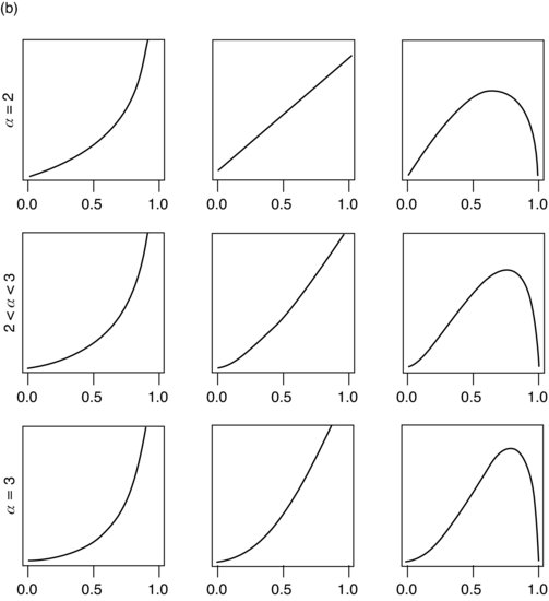
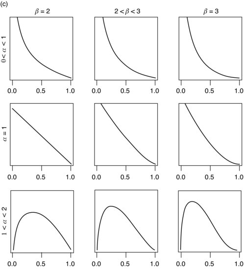
The family of beta distributions is illustrated in Figure 3.1. Basically, any reasonably smooth unimodal distribution on [0, 1] is likely to be reasonably well approximated by some beta distribution, so that it is very often possible to approximate your prior beliefs by a member of the conjugate family, with all the simplifications that this implies. In identifying an appropriate member of the family, it is often useful to equate the mean

of to a value which represents your belief and to a number which in some sense represents the number of observations which you reckon your prior information to be worth. (It is arguable that it should be or that should equal this number, but in practice this will make no real difference). Alternatively, you could equate the mean to a value which represents your beliefs about the location of π and the variance

of to a value which represents how spread out your beliefs are.

3.1.2 Odds and log-odds

We sometimes find it convenient to work in terms of the odds on success against failure, defined by

so that . One reason for this is the relationship mentioned in Appendix A that if then

has Snedecor’s F distribution. Moreover, the log-odds

is close to having Fisher’s z distribution; more precisely

It is then easy to deduce from the properties of the z distribution given in Appendix A that

One reason why it is useful to consider the odds and log-odds is that tables of the F and z distributions are more readily available than tables of the beta distribution.

3.1.3 Highest density regions

Tables of HDRs of the beta distribution are available [see, Novick and Jackson (1974, Table A.15) or Isaacs et al. (1974, Table 43)], but it is not necessary or particularly desirable to use them. (The reason is related to the reason for not using HDRs for the inverse chi-squared distribution as such.) In Section 3.2, we shall discuss the choice of a reference prior for the unknown parameter π. It turns out that there are several possible candidates for this honour, but there is at least a reasonably strong case for using a prior

Using the usual change-of-variable rule , it is easily seen that this implies a uniform prior

in the log-odds Λ. As argued in Section 2.8 on ‘HDRs for the normal variance’, this would seem to be an argument in favour of using an interval in which the posterior distribution of is higher than anywhere outside. The Appendix includes tables of values of F corresponding to HDRs for log F, and the distribution of Λ as deduced earlier is clearly very nearly that of log F. Hence in seeking for, for example, a 90% interval for π when , we should first look up values and corresponding to a 90% HDR for . Then a suitable interval for values of the odds λ is given by

from which it follows that a suitable interval of values of π is

If the tables were going to be used solely for this purpose, they could be better arranged to avoid some of the arithmetic involved at this stage, but as they are used for other purposes and do take a lot of space, the minimal extra arithmetic is justifiable.

Although this is not the reason for using these tables, a helpful thing about them is that we need not tabulate values of and for . This is because if F has an distribution then F–1 has an distribution. It follows that if an HDR for log F is then an HDR for log F–1 is , and so if is replaced by then the interval is simply replaced by . There is no such simple relationship in tables of HDRs for F itself or in tables of HDRs for the beta distribution.

3.1.4 Example

It is my guess that about 20% of the best known (printable) limericks have the same word at the end of the last line as at the end of the first. However, I am not very sure about this, so I would say that my prior information was only ‘worth’ some nine observations. If I seek a conjugate prior to represent my beliefs, I need to take

These equations imply that and . There is no particular reason to restrict α and β to integer values, but on the other hand prior information is rarely very precise, so it seems simpler to take and . Having made these conjectures, I then looked at one of my favourite books of light verse, Silcock (1952), and found that it included 12 limericks, of which two (both by Lear) have the same word at the ends of the first and last lines. This leads me to a posterior which is Be(4, 17). I can obtain some idea of what this distribution is like by looking for a 90% HDR. From interpolation in the tables in the Appendix, values of F corresponding to a 90% HDR for log F34,8 are and . It follows that an appropriate interval of values of F8,34 is , that is (0.35, 2.38), so that an appropriate interval for π is

that is (0.08, 0.36).

If for some reason, we want HDRs for π itself, instead of for and insist on using HDRs for π itself, then we can use the tables quoted earlier [namely, Novick and Jackson (1974, Table A.15) or Isaacs et al. (1974, Table 43)]. Alternatively, Novick and Jackson (1974, Section 5.5), point out that a reasonable approximation can be obtained by finding the median of the posterior distribution and looking for a 90% interval such that the probability of being between the lower bound and the median is 45% and the probability of being between the median and the upper bound is 45%. The usefulness of this procedure lies in the ease with which it can be followed using tables of the percentage points of the beta distribution alone, should tables of HDRs be unavailable. It can even be used in connection with the nomogram which constitutes Table 17 of Pearson and Hartley (ed.) (1966), although the accuracy resulting leaves something to be desired. On the whole, the use of the tables of values of F corresponding to HDRs for log F, as described earlier, seems preferable.

3.1.5 Predictive distribution

The posterior distribution is clearly of the form for some α and β (which, of course, include x and n–x, respectively), so that the predictive distribution of the next observation after we have the single observation x on top of our previous background information is

This distribution is known as the beta-binomial distribution,or sometimes as the Pólya distribution [see Calvin, 1984]. We shall not have a great deal of use for it in this book, although we will refer to it briefly in Chapter 9. It is considered, for example, in Raiffa and Schlaifer (1961, Section 7.11). We shall encounter a related distribution, the beta-Pascal distribution in Section 7.3 when we consider informative stopping rules.