Excel offers a fairly robust object model for PivotTables. You can use the macro recorder to create a macro that does just about anything with a PivotTable, and the macro gets you 90 percent of the way to automation. For instance, you can record a macro that builds a PivotTable, and that macro records your steps and duplicates your tasks with relatively high fidelity. So if you find yourself needing to automate tasks like filtering out the top 10 items or grouping data items, you can reliably turn to the macro recorder to help write the VBA needed.
That being said, certain PivotTable-related tasks are not easily solved with the macro recorder. This is what this Part focuses on. Here, we cover the most common scenarios where macros help you gain efficiencies when working with PivotTables.
 The code for this Part can be found on this book's companion website. See this book's Introduction for more on the companion website.
Macro 62: Create a Backwards-Compatible PivotTable
If you are still using Excel 2003, you may know about the compatibility headaches that come with PivotTables between Excel 2003 and later versions. As you can imagine, the extraordinary increases in PivotTable limitations lead to some serious compatibility questions. For instance, later versions of Excel PivotTables can have more than 16,384 column fields and more than 1,000,000 unique data items. Excel 2003 can have only 256 column fields and 32,500 unique data items.
To solve these compatibility issues, Microsoft has initiated the concept of Compatibility mode. Compatibility mode is a state that Excel automatically enters when opening an xls file. When Excel is in Compatibility mode, it artificially takes on the limitations of Excel 2003. This means while you are working with an xls file, you cannot exceed any of the Excel 2003 PivotTable limitations, allowing you (as a user of Excel 2007 or 2010) to create PivotTables that work with Excel 2003.
If you are not in Compatibility mode (meaning you are working with an xlsx or xlsm file) and you create a PivotTable, the PivotTable object turns into a hard table when opened in Excel 2003. That is to say, PivotTables that are created in xlsx or xlsm files are destroyed when opened in Excel 2003.
To avoid this fiasco manually, Excel 2007 and 2010 users must go through these steps:
1. Create a blank workbook.
2. Save the file as an xls file.
3. Close the file.
4. Open it up again.
5. Start creating the PivotTable.
This is enough to drive you up the wall if you've got to do this every day.
An alternative is to use a macro that automatically starts a PivotTable in Table in the Excel 2003 version — even if you are not in Compatibility mode!
How it works
If you record a macro while creating a PivotTable in Excel 2007 or Excel 2010, the macro recorder generates the code to create your PivotTable. This code has several arguments in it. One of the arguments is the Version property. As the name implies, the Version property specifies the version of Excel the PivotTable was created in. The nifty thing is that you can change the Version in the code to force Excel to create a PivotTable that will work with Excel 2003.
Here is a listing of the different versions you can specify:
• xlPivotTableVersion2000 - Excel 2000
• xlPivotTableVersion10 - Excel 2002
• xlPivotTableVersion11 - Excel 2003
• xlPivotTableVersion12 - Excel 2007
• xlPivotTableVersion14 - Excel 2010
Here is an example of a macro that starts a PivotTable using Range(“A3:N86”) on Sheet1 as the source data.
Note that we changed the Version and DefaultVersion properties to xlPivotTableVersion11. This ensures that the PivotTable starts off as one that will work in Excel 2003.
No need to save your workbook as an .xls file first or to be in Compatibility mode. You can use a simple macro like this (just change the source data range) to create a PivotTable that will automatically work with Excel 2003.
Sub Macro62()
Dim SourceRange As Range
Set SourceRange = Sheets(“Sheet1”).Range(“A3:N86”)
ActiveWorkbook.PivotCaches.Create( _
SourceType:=xlDatabase, _
SourceData:=SourceRange, _
Version:=xlPivotTableVersion11).CreatePivotTable _
TableDestination:=””, _
TableName:=””, _
DefaultVersion:=xlPivotTableVersion11
End Sub
 Keep in mind that creating a PivotTable in the Excel 2003 version will essentially force the PivotTable to take on the limits of Excel 2003. This means any new PivotTable limit increases or PivotTable features added in Excel 2007 or Excel 2010 will not be available in your 2003 version PivotTable.
How to use it
To implement this macro, you can copy and paste it into a standard module:
1. Activate the Visual Basic Editor by pressing ALT+F11.
2. Right-click the project/workbook name in the Project window.
3. Choose Insert⇒Module.
4. Type or paste the code.
Macro 63: Refresh All PivotTables Workbook
It's not uncommon to have multiple PivotTables in the same workbook. Many times, these PivotTables link to data that changes, requiring a refresh of the PivotTables. If you find that you need to refresh your PivotTables en masse, you can use this macro to refresh all PivotTables on demand.
How it works
It's important to know that each PivotTable object is a child of the worksheet it sits in. The macro has to first loop through the worksheets in a workbook first, and then loop through the PivotTables in each worksheet. This macro does just that — loops through the worksheets, and then loops through the PivotTables. On each loop, the macro refreshes the PivotTable.
Sub Macro63()
‘Step 1: Declare your Variables
Dim ws As Worksheet
Dim pt As PivotTable
‘Step 2: Loop through each sheet in workbook
For Each ws In ThisWorkbook.Worksheets
‘Step 3: Loop through each PivotTable
For Each pt In ws.PivotTables
pt.RefreshTable
Next pt
Next ws
End Sub
1. Step 1 first declares an object called ws. This creates a memory container for each worksheet we loop through. It also declares an object called pt, which holds each PivotTable the macro loops through.
2. Step 2 starts the looping, telling Excel we want to evaluate all worksheets in this workbook. Notice we are using ThisWorkbook instead of ActiveWorkbook. The ThisWorkbook object refers to the workbook that the code is contained in. The ActiveWorkbook object refers to the workbook that is currently active. They often return the same object, but if the workbook running the code is not the active workbook, they return different objects. In this case, we don't want to risk refreshing PivotTables in other workbooks, so we use ThisWorkbook.
3. Step 3 loops through all the PivotTables in each worksheet, and then triggers the RefreshTable method. After all PivotTables have been refreshed, the macro moves to the next sheet. After all sheets have been evaluated, the macro ends.
As an alternative method for refreshing all PivotTables in the workbook, you can use ThisWorkbook.RefreshAll. This refreshes all the PivotTables in the workbook. However, it also refreshes all query tables. So if you have data tables that are connected to an external source or the web, these will be affected by the RefreshAll method. If this is not a concern, you can simply enter ThisWorkbook.RefreshAll into a standard module.
How to use it
To implement this macro, you can copy and paste it into a standard module:
1. Activate the Visual Basic Editor by pressing ALT+F11.
2. Right-click the project/workbook name in the Project window.
3. Choose Insert⇒Module.
4. Type or paste the code.
Macro 64: Create a PivotTable Inventory Summary
When your workbook contains multiple PivotTables, it's often helpful to have an inventory summary (similar to the one shown here in Figure 6-1) that outlines basic details about the PivotTables. With this type of summary, you can quickly see important information like the location of each PivotTable, the location of each PivotTable's source data, and the pivot cache index each PivotTable is using.

Figure 6-1: A PivotTable inventory summary.
The following macro outputs such a summary.
How it works
When you create a PivotTable object variable, you expose all of a PivotTable's properties — properties like its name, location, cache index, and so on. In this macro, we loop through each PivotTable in the workbook and extract specific properties into a new worksheet.
Because each PivotTable object is a child of the worksheet it sits in, we have to first loop through the worksheets in a workbook first, and then loop through the PivotTables in each worksheet.
Take a moment to walk through the steps of this macro in detail.
Sub Macro64()
‘Step 1: Declare your Variables
Dim ws As Worksheet
Dim pt As PivotTable
Dim MyCell As Range
‘Step 2: Add a new sheet with column headers
Worksheets.Add
Range(“A1:F1”) = Array(“Pivot Name”, “Worksheet”, _
“Location”, “Cache Index”, _
“Source Data Location”, _
“Row Count”)
‘Step 3: Start Cursor at Cell A2 setting the anchor here
Set MyCell = ActiveSheet.Range(“A2”)
‘Step 4: Loop through each sheet in workbook
For Each ws In Worksheets
‘Step 5: Loop through each PivotTable
For Each pt In ws.PivotTables
MyCell.Offset(0, 0) = pt.Name
MyCell.Offset(0, 1) = pt.Parent.Name
MyRange.Offset(0, 2) = pt.TableRange2.Address
MyRange.Offset(0, 3) = pt.CacheIndex
MyRange.Offset(0, 4) = Application.ConvertFormula _
(pt.PivotCache.SourceData, xlR1C1, xlA1)
MyRange.Offset(0, 5) = pt.PivotCache.RecordCount
‘Step 6: Move Cursor down one row and set a new anchor
Set MyRange = MyRange.Offset(1, 0)
‘Step 7: Work through all PivotTables and worksheets
Next pt
Next ws
‘Step 8: Size columns to fit
ActiveSheet.Cells.EntireColumn.AutoFit
End Sub
1. Step 1 declares an object called ws. This creates a memory container for each worksheet we loop through. We then declare an object called pt, which holds each PivotTable we loop through. Finally, we create a range variable called MyCell. This variable acts as our cursor as we fill in the inventory summary.
2. Step 2 creates a new worksheet and adds column headings that range from A1 to F1. Note that we can add column headings using a simple array that contains our header labels. This new worksheet remains our active sheet from here on out.
3. Just as you would manually place your cursor in a cell if you were to start typing data, Step 3 places the MyCell cursor in cell A2 of the active sheet. This is our anchor point, allowing us to navigate from here.
Throughout the macro, you see the use of the Offset property. The Offset property allows us to move a cursor x number of rows and x number of columns from an anchor point. For instance, Range(A2).Offset(0,1) would move the cursor one column to the right. If we wanted to move the cursor one row down, we would enter Range(A2).Offset(1, 0).
In the macro, we navigate by using Offset on MyCell. For example, MyCell.Offset(0,4) would move the cursor four columns to the right of the anchor cell. After the cursor is in place, we can enter data.
4. Step 4 starts the looping, telling Excel we want to evaluate all worksheets in this workbook.
5. Step 5 loops through all the PivotTables in each worksheet. For each PivotTable it finds, it extracts out the appropriate property and fills in the table based on the cursor position (see Step 3).
We are using six PivotTable properties: Name, Parent.Range, TableRange2.Address, CacheIndex, PivotCache.SourceData, and PivotCache.Recordcount.
The Name property returns the name of the PivotTable.
The Parent.Range property gives us the sheet where the PivotTable resides. The TableRange2.Address property returns the range that the PivotTable object sits in.
The CacheIndex property returns the index number of the pivot cache for the PivotTable. A pivot cache is a memory container that stores all the data for a PivotTable. When you create a new PivotTable, Excel takes a snapshot of the source data and creates a pivot cache. Each time you refresh a PivotTable, Excel goes back to the source data and takes another snapshot, thereby refreshing the pivot cache. Each pivot cache has a SourceData property that identifies the location of the data used to create the pivot cache. The PivotCache.SourceData property tells us which range will be called upon when we refresh the PivotTable. You can also pull out the record count of the source data by using the PivotCache.Recordcount property.
6. Each time the macro encounters a new PivotTable, it moves the MyCell cursor down a row, effectively starting a new row for each PivotTable.
7. Step 7 tells Excel to loop back around to iterate through all PivotTables and all worksheets. After all PivotTables have been evaluated, we move to the next sheet. After all sheets have been evaluated, the macro moves to the last step.
8. Step 8 finishes off with a little formatting, sizing the columns to fit the data.
How to use it
To implement this macro, you can copy and paste it into a standard module:
1. Activate the Visual Basic Editor by pressing ALT+F11.
2. Right-click the project/workbook name in the Project window.
3. Choose Insert⇒Module.
4. Type or paste the code.
Macro 65: Make All PivotTables Use the Same Pivot Cache
If you work with PivotTables enough, you will undoubtedly find the need to analyze the same dataset in multiple ways. In most cases, this process requires you to create separate PivotTables from the same data source.
The problem is that each time you create a PivotTable, you are storing a snapshot of the data source in a pivot cache. Every pivot cache that is created increases your memory usage and file size. The side effect of this behavior is that your spreadsheet bloats with redundant data. Making your PivotTables share the same cache prevents this.
Starting with Excel 2007, Microsoft built in an automatic pivot cache sharing algorithm that recognizes when you are creating a PivotTable from the same source as an existing PivotTable. This reduces the instances of creating superfluous pivot caches. However, you can still inadvertently create multiple pivot caches if the number of rows or columns captured from your source range is different for each of your PivotTables.
In addition to the reduction in file size, there are other benefits to sharing a pivot cache:
• You can refresh one PivotTable and all others that share the pivot cache are refreshed also.
• When you add a Calculated Field to one PivotTable, your newly created calculated field shows up in the other PivotTables' field list.
• When you add a Calculated Item to one PivotTable, it shows up in the others as well.
• Any grouping or ungrouping you perform affects all PivotTables sharing the same cache.
How it works
With the last macro, you are able to take an inventory of all your PivotTables. In that inventory summary, you can see the pivot cache index of each PivotTable (see Figure 6-1). Using this, you can determine which PivotTable contains the most appropriate pivot cache, and then force all others to share the same cache.
In this example, we are forcing all PivotTables to the pivot cache used by PivotTable1 on the Units Sold sheet.
Sub Macro65()
‘Step 1: Declare your Variables
Dim ws As Worksheet
Dim pt As PivotTable
‘Step 2: Loop through each sheet in workbook
For Each ws In ThisWorkbook.Worksheets
‘Step 3: Loop through each PivotTable
For Each pt In ws.PivotTables
pt.CacheIndex = _
Sheets(“Units Sold”).PivotTables(“PivotTable1”).CacheIndex
Next pt
Next ws
End Sub
1. Step 1 declares an object called ws. This creates a memory container for each worksheet we loop through. We also declare an object called pt, which holds each PivotTable we loop through.
2. Step 2 starts the looping, telling Excel we want to evaluate all worksheets in this workbook. Notice we are using ThisWorkbook instead of ActiveWorkbook. ThisWorkbook object refers to the workbook that the code is contained in. ActiveWorkbook object refers to the workbook that is currently active. They often return the same object, but if the workbook running the code is not the active workbook, they return different objects. In this case, we don't want to risk affecting PivotTables in other workbooks, so we use ThisWorkbook.
3. Step 3 loops through all the PivotTables in each worksheet, and then sets the CachIndex to the same one used by PivotTable1 on the “Units Sold” sheet. After all PivotTables have been refreshed, we move to the next sheet. After all sheets have been evaluated, the macro ends.
How to use it
To implement this macro, you can copy and paste it into a standard module:
1. Activate the Visual Basic Editor by pressing ALT+F11.
2. Right-click the project/workbook name in the Project window.
3. Choose Insert⇒Module.
4. Type or paste the code.
Macro 66: Hide All Subtotals in a PivotTable
When you create a PivotTable, Excel includes subtotals by default. This inevitably leads to a PivotTable report that inundates the eyes with all kinds of numbers, making it difficult to analyze. Figure 6-2 demonstrates this.

Figure 6-2: Subtotals can sometimes hinder analysis.
Manually removing Subtotals is easy enough; right-click the field headers and uncheck the Subtotal option. But if you're constantly hiding subtotals, you can save a little time by automating the process with a simple macro.
You can manually hide all subtotals at once by going to the Ribbon and selecting PivotTable Tools⇒Design⇒Layout⇒Subtotals⇒Do Not Show Subtotals. But again, if you are building an automated process that routinely manipulates pivot tables without manual intervention, you may prefer the macro option.
How it works
If you record a macro while hiding a Subtotal in a PivotTable, Excel produces code similar to this:
ActiveSheet.PivotTables(“Pvt1″).PivotFields(“Region”).Subtotals = Array(False, False, False, False, False, False, False, False, False, False, False, False)
That's right; Excel passes an array with exactly 12 False settings. There are 12 instances of False because there are twelve types of Subtotals — Sum, Avg, Count, Min, and Max, just to name a few. So when you turn off Subtotals while recording a macro, Excel sets each of the possible Subtotal types to False.
An alternative way of turning off Subtotals is to first set one of the 12 Subtotals to True. This automatically forces the other 11 Subtotal types to False. We then set the same Subtotal to False, effectively hiding all Subtotals. In this piece of code, we are setting the first Subtotal to True, and then setting it to False. This removes the subtotal for Region.
With ActiveSheet.PivotTables(“Pvt1″).PivotFields(“Region”)
.Subtotals(1) = True
.Subtotals(1) = False
End With
In our macro, we use this trick to turn off subtotals for every pivot field in the active PivotTable.
Sub Macro66()
‘Step 1: Declare your Variables
Dim pt As PivotTable
Dim pf As PivotField
‘Step 2: Point to the PivotTable in the active cell
On Error Resume Next
Set pt = ActiveSheet.PivotTables(ActiveCell.PivotTable.Name)
‘Step 3: Exit if active cell is not in a PivotTable
If pt Is Nothing Then
MsgBox “You must place your cursor inside of a PivotTable.”
Exit Sub
End If
‘Step 4: Loop through all pivot fields and remove totals
For Each pf In pt.PivotFields
pf.Subtotals(1) = True
pf.Subtotals(1) = False
Next pf
End Sub
1. Step 1 declares two object variables. This macro uses pt as the memory container for the PivotTable and uses pf as a memory container for the pivot fields. This allows us to loop through all the pivot fields in the PivotTable.
2. This macro is designed so that we infer the active PivotTable based on the active cell. That is to say, the active cell must be inside a PivotTable for this macro to run. The assumption is that when the cursor is inside a particular PivotTable, we want to perform the macro action on that pivot.
Step 2 sets the pt variable to the name of the PivotTable on which the active cell is found. We do this by using the ActiveCell.PivotTable.Name property to get the name of the target pivot.
If the active cell is not inside of a PivotTable, an error is thrown. This is why the macro uses the On Error Resume Next statement. This tells Excel to continue with the macro if there is an error.
3. Step 3 checks to whether the pt variable is filled with a PivotTable object. If the pt variable is set to Nothing, the active cell was not on a PivotTable, thus no PivotTable could be assigned to the variable. If this is the case, we tell the user in a message box, and then we exit the procedure.
4. If the macro reaches Step 4, it has successfully pointed to a PivotTable. We are ready to loop to all the fields in the PivotTable. We use a For Each statement to iterate through each pivot field. Each time a new pivot field is selected, we apply our Subtotal logic. After all the fields have been evaluated, the macro ends.
How to use it
To implement this macro, you can copy and paste it into a standard module:
1. Activate the Visual Basic Editor by pressing ALT+F11.
2. Right-click the project/workbook name in the Project window.
3. Choose Insert⇒Module.
4. Type or paste the code.
Macro 67: Adjust All Pivot Data Field Titles
When you create a PivotTable, Excel tries to help you out by prefacing each data field header with Sum of, Count of, or whichever operation you use. Often, this is not conducive to your reporting needs. You want clean titles that match your data source as closely as possible. Although it's true that you can manually adjust the titles for you data fields (one at a time), this macro fixes them all in one go.
How it works
Ideally, the name of the each data item matches the field name from your source data set (the original source data used to create the PivotTable). Unfortunately, PivotTables won't allow you to name a data field the exact name as the source data field. The workaround for this is to add a space to the end of the field name. Excel considers the field name (with a space) to be different from the source data field name, so it allows it. Cosmetically, the readers of your spreadsheet don't notice the space after the name.
This macro utilizes this workaround to rename your data fields. It loops through each data field in the PivotTable, and then resets each header to match its respective field in the source data plus a space character.
Sub Macro67()
‘Step 1: Declare your Variables
Dim pt As PivotTable
Dim pf As PivotField
‘Step 2: Point to the PivotTable in the active cell
On Error Resume Next
Set pt = ActiveSheet.PivotTables(ActiveCell.PivotTable.Name)
‘Step 3: Exit if active cell is not in a PivotTable
If pt Is Nothing Then
MsgBox “You must place your cursor inside of a PivotTable.”
Exit Sub
End If
‘Step 4: Loop through all pivot fields adjust titles
For Each pf In pt.DataFields
pf.Caption = pf.SourceName & Chr(160)
Next pf
End Sub
1. Step 1 declares two object variables. It uses pt as the memory container for our PivotTable and pf as a memory container for the data fields. This allows the macro to loop through all the data fields in the PivotTable.
2. This macro is designed so that we infer the active PivotTable based on the active cell. In other words, the active cell must be inside a PivotTable for this macro to run. We assume that when the cursor is inside a particular PivotTable, we want to perform the macro action on that pivot.
Step 2 sets the pt variable to the name of the PivotTable on which the active cell is found. We do this by using the ActiveCell.PivotTable.Name property to get the name of the target pivot.
If the active cell is not inside of a PivotTable, an error is thrown. This is why we use the On Error Resume Next statement. This tells Excel to continue with the macro if there is an error.
3. In Step 3, we check to see if the pt variable is filled with a PivotTable object. If the pt variable is set to Nothing, the active cell was not on a PivotTable, thus no PivotTable could be assigned to the variable. If this is the case, we tell the user in a message box, and then we exit the procedure.
4. If the macro reaches Step 4, it has successfully pointed to a PivotTable. The macro uses a For Each statement to iterate through each data field. Each time a new pivot field is selected, the macro changes the field name by setting the Caption property to match the field's SourceName. The SourceName property returns the name of the matching field in the original source data.
To that name, the macro concatenates a non-breaking space character: Chr(160).
Every character has an underlying ASCII code, similar to a serial number. For instance, the lowercase letter a has an ASCII code of 97. The lowercase letter c has an ASCII code of 99. Likewise, invisible characters such as the space have a code. You can use invisible characters in your macro by passing their code through the CHR function.
After the name has been changed, the macro moves to the next data field. After all the data fields have been evaluated, the macro ends.
How to use it
To implement this macro, you can copy and paste it into a standard module:
1. Activate the Visual Basic Editor by pressing ALT+F11.
2. Right-click the project/workbook name in the Project window.
3. Choose Insert⇒Module.
4. Type or paste the code.
Macro 68: Set All Data Items to Sum
When creating a PivotTable, Excel, by default, summarizes your data by either counting or summing the items. The logic Excel uses to decide whether to sum or count the fields you add to your PivotTable is fairly simple. If all of the cells in a column contain numeric data, Excel chooses to Sum. If the field you are adding contains a blank or text, Excel chooses Count.
Although this seems to make sense, in many instances, a pivot field that should be summed legitimately contains blanks. In these cases, we are forced to manually go in after Excel and change the calculation type from Count back to Sum. That's if we're paying attention! It's not uncommon to miss the fact that a pivot field is being counted instead of summed up.
The macro in this section aims to help by automatically setting each data item's calculation type to Sum.
How it works
This macro loops through each data field in the PivotTable and changes the Function property to xlSum. You can alter this macro to use any one of the calculation choices: xlCount, xlAverage, xlMin, xlMax, and so on. When you go into the code window and type pf.Function =, you see a drop-down list showing you all your choices (see Figure 6-3).

Figure 6-3: Excel helps out by showing you your enumeration choices.
Sub Macro68()
‘Step 1: Declare your Variables
Dim pt As PivotTable
Dim pf As PivotField
‘Step 2: Point to the PivotTable in the active cell
On Error Resume Next
Set pt = ActiveSheet.PivotTables(ActiveCell.PivotTable.Name)
‘Step 3: Exit if active cell is not in a PivotTable
If pt Is Nothing Then
MsgBox “You must place your cursor inside of a PivotTable.”
Exit Sub
End If
‘Step 4: Loop through all pivot fields apply SUM
For Each pf In pt.DataFields
pf.Function = xlSum
Next pf
End Sub
1. Step 1 declares two object variables. It uses pt as the memory container for the PivotTable and pf as a memory container for the data fields. This allows us to loop through all the data fields in the PivotTable.
2. This macro is designed so that we infer the active PivotTable based on the active cell. The active cell must be inside a PivotTable for this macro to run. The assumption is that when the cursor is inside a particular PivotTable, we want to perform the macro action on that pivot.
Step 2 sets the pt variable to the name of the PivotTable on which the active cell is found. We do this by using the ActiveCell.PivotTable.Name property to get the name of the target pivot.
If the active cell is not inside of a PivotTable, an error is thrown. This is why we use the On Error Resume Next statement. This tells Excel to continue with the macro if there is an error.
3. Step 3 checks to see if the pt variable is filled with a PivotTable object. If the pt variable is set to Nothing, the active cell was not on a PivotTable, thus no PivotTable could be assigned to the variable. If this is the case, we tell the user in a message box, and then we exit the procedure.
4. If the macro has reached Step 4, it has successfully pointed to a PivotTable. It uses a For Each statement to iterate through each data field. Each time a new pivot field is selected, it alters the Function property to set the calculation used by the field. In this case, we are setting all the data fields in the PivotTable to Sum.
After the name has been changed, we move to the next data field. After all the data fields have been evaluated, the macro ends.
How to use it
To implement this macro, you can copy and paste it into a standard module:
1. Activate the Visual Basic Editor by pressing ALT+F11.
2. Right-click the project/workbook name in the Project window.
3. Choose Insert⇒Module.
4. Type or paste the code.
Macro 69: Apply Number Formatting for All Data Items
A PivotTable does not inherently store number formatting in its pivot cache. Formatting takes up memory; so in order to be as lean as possible, the pivot cache only contains data. Unfortunately, this results in the need to apply number formatting to every field you add to a PivotTable. This takes from eight to ten clicks of the mouse for every data field you add. When you have PivotTables that contain five or more data fields, you're talking about more than 40 clicks of the mouse!
Ideally, a PivotTable should be able to look back at its source data and adopt the number formatting from the fields there. The macro outlined in this section is designed to do just that. It recognizes the number formatting in the PivotTable's source data and applies the appropriate formatting to each field automatically.
How it works
Before running this code, you want to make sure that
• The source data for your PivotTable is accessible. The macro needs to see it in order to capture the correct number formatting.
• The source data is appropriately formatted. Money fields are formatted as currency, value fields are formatted as numbers, and so on.
This macro uses the PivotTable SourceData property to find the location of the source data. It then loops through each column in the source, capturing the header name and the number format of the first value under each column. After it has that information, the macro determines whether any of the data fields match the evaluated column. If it finds a match, the number formatting is applied to that data field.
Sub Macro69()
‘Step 1: Declare your Variables
Dim pt As PivotTable
Dim pf As PivotField
Dim SrcRange As Range
Dim strFormat As String
Dim strLabel As String
Dim i As Integer
‘Step 2: Point to the PivotTable in the activecell
On Error Resume Next
Set pt = ActiveSheet.PivotTables(ActiveCell.PivotTable.Name)
‘Step 3: Exit if active cell is not in a PivotTable
If pt Is Nothing Then
MsgBox “You must place your cursor inside of a PivotTable.”
Exit Sub
End If
‘Step 4: Capture the source range
Set SrcRange = _
Range(Application.ConvertFormula(pt.SourceData, xlR1C1, xlA1))
‘Step 5: Start looping through the columns in source range
For i = 1 To SrcRange.Columns.Count
‘Step 6: Trap the source column name and number format
strLabel = SrcRange.Cells(1, i).Value
strFormat = SrcRange.Cells(2, i).NumberFormat
‘Step 7: Loop through the fields PivotTable data area
For Each pf In pt.DataFields
‘Step 8: Check for match on SourceName then apply format
If pf.SourceName = strLabel Then
pf.NumberFormat = strFormat
End If
Next pf
Next i
End Sub
1. Step 1 declares six variables. It uses pt as the memory container for our PivotTable and pf as a memory container for our data fields. The SrcRange variable holds the data range for the source data. The strFormat and strLabel variables are both text string variables used to hold the source column label and number formatting respectively. The i variable serves as a counter, helping us enumerate through the columns of the source data range.
2. The active cell must be inside a PivotTable for this macro to run. The assumption is that when the cursor is inside a particular PivotTable, we want to perform the macro action on that pivot.
Step 2 sets the pt variable to the name of the PivotTable on which the active cell is found. We do this by using the ActiveCell.PivotTable.Name property to get the name of the target pivot.
If the active cell is not inside a PivotTable, an error is thrown. This is why the macro uses the On Error Resume Next statement. This tells Excel to continue with the macro if there is an error.
3. Step 3 checks to see whether the pt variable is filled with a PivotTable object. If the pt variable is set to Nothing, the active cell was not on a PivotTable, thus no PivotTable could be assigned to the variable. If this is the case, we tell the user in a message box, and then we exit the procedure.
4. If the macro reaches Step 4, it has successfully pointed to a PivotTable. We immediately fill our SrcRange object variable with the PivotTable's source data range.
All PivotTables have a SourceData property that points to the address of its source. Unfortunately, the address is stored in the R1C1 reference style — like this: ‘Raw Data'!R3C1:R59470C14. Range objects cannot use the R1C1 style, so we need the address to be converted to ‘Raw Data'!$A$3:$N$59470.
This is a simple enough fix. We simply pass the SourceData property through the Application.ConvertFormula function. This handy function converts ranges to and from the R1C1 reference style.
5. After the range is captured, the macro starts looping through the columns in the source range. In this case, we manage the looping by using the i integer as an index number for the columns in the source range. We start the index number at 1 and end it at the maximum number of rows in the source range.
6. As the macro loops through the columns in the source range, we capture the column header label and the column format.
We do this with the aid of the Cells item. The Cells item gives us an extremely handy way of selecting ranges through code. It requires only relative row and column positions as parameters. Cells(1,1) translates to row 1, column 1 (or the header row of the first column). Cells(2, 1) translates to row 2, column 1 (or the first value in the first column).
strLabel is filled by the header label taken from row 1 of the column that is selected. strFormat is filled with the number formatting from row 2 of the column that is selected.
7. At this point, the macro has connected with the PivotTable's source data and captured the first column name and number formatting for that column. Now it starts looping through the data fields in the PivotTable.
8. Step 8 simply compares each data field to see if its source matches the name in strLabel. If it does, that means the number formatting captured in strFormat belongs to that data field.
9. After all data fields have been evaluated, the macro increments i to the next column in the source range. After all columns have been evaluated, the macro ends.
How to use it
To implement this macro, you can copy and paste it into a standard module:
1. Activate the Visual Basic Editor by pressing ALT+F11.
2. Right-click project/workbook name in the Project window.
3. Choose Insert⇒Module.
4. Type or paste the code.
Macro 70: Sort All Fields in Alphabetical Order
If you frequently add data to your PivotTables, you may notice that new data doesn't automatically fall into the sort order of the existing pivot data. Instead, it gets tacked to the bottom of the existing data. This means that your drop-down lists show all new data at the very bottom, whereas existing data is sorted alphabetically.
How it works
This macro works to reset the sorting on all data fields, ensuring that any new data snaps into place. The idea is to run it each time you refresh your PivotTable. In the code, we enumerate through each data field in the PivotTable, sorting each one as we go.
Sub Macro70()
‘Step 1: Declare your Variables
Dim pt As PivotTable
Dim pf As PivotField
‘Step 2: Point to the PivotTable in the activecell
On Error Resume Next
Set pt = ActiveSheet.PivotTables(ActiveCell.PivotTable.Name)
‘Step 3: Exit if active cell is not in a PivotTable
If pt Is Nothing Then
MsgBox “You must place your cursor inside of a PivotTable.”
Exit Sub
End If
‘Step 4: Loop through all pivot fields and sort
For Each pf In pt.PivotFields
pf.AutoSort xlAscending, pf.Name
Next pf
End Sub
1. Step 1 declares two object variables, using pt as the memory container for the PivotTable and using pf as a memory container for our data fields. This allows the macro to loop through all the data fields in the PivotTable.
2. The active cell must be inside a PivotTable for this macro to run. The assumption is that when the cursor is inside a particular PivotTable, we want to perform the macro action on that pivot.
In Step 2, we set the pt variable to the name of the PivotTable on which the active cell is found. We do this by using the ActiveCell.PivotTable.Name property to get the name of the target pivot.
If the active cell is not inside of a PivotTable, an error is thrown. This is why we use the On Error Resume Next statement. This tells Excel to continue with the macro if there is an error.
3. Step 3 checks to see whether the pt variable is filled with a PivotTable object. If the pt variable is set to Nothing, the active cell was not on a PivotTable, thus no PivotTable could be assigned to the variable. If this is the case, the macro puts up a message box to notify the user, and then exits the procedure.
4. Finally, we use a For Each statement to iterate through each pivot field. Each time a new pivot field is selected, we use the AutoSort method to reset the automatic sorting rules for the field. In this case, we are sorting all fields in ascending order. After all the data fields have been evaluated, the macro ends.
How to use it
To implement this macro, you can copy and paste it into a standard module:
1. Activate the Visual Basic Editor by pressing ALT+F11.
2. Right-click the project/workbook name in the Project window.
3. Choose Insert⇒Module.
4. Type or paste the code.
Macro 71: Apply Custom Sort to Data Items
On occasion, you may need to apply a custom sort to the data items in your PivotTable. For instance, if you work for a company in California, your organization may want the West region to come before the North and South. In these types of situations, neither the standard ascending nor descending sort order will work.
How it works
You can automate the custom sorting of your fields by using the Position property of the PivotItems object. With the Position property, you can assign a position number that specifies the order in which you would like to see each pivot item.
In this example code, we first point to the Region pivot field in the Pvt1 PivotTable. Then we list each item along with the position number indicating the customer sort order we need.
Sub Macro71()
With Sheets(“Sheet1”).PivotTables(“Pvt1”).PivotFields(“Region “)
.PivotItems(“West”).Position = 1
.PivotItems(“North”).Position = 2
.PivotItems(“South”).Position = 3
End With
End Sub
The other solution is to set up a custom sort list. A custom sort list is a defined list that is stored in your instance of Excel. To create a custom sort list, go to the Excel Options dialog box and choose Edit Custom Lists. Here, you can type West, North, and South in the List Entries box and click Add. After setting up a custom list, Excel realizes that the Region data items in your PivotTable match a custom list and sorts the field to match your custom list.
As brilliant as this option is, custom lists do not travel with your workbook, so a macro helps in cases where it's impractical to expect your clients or team members to set up their own custom sort lists.
How to use it
You can implement this kind of a macro in a standard module:
1. Activate the Visual Basic Editor by pressing ALT+F11.
2. Right-click the project/workbook name in the Project window.
3. Choose Insert⇒Module.
4. Type or paste the code.
Macro 72: Apply PivotTable Restrictions
We often send PivotTables to clients, coworkers, managers, and other groups of people. In some cases, we'd like to restrict the types of actions our users can take on the PivotTable reports we send them. The macro outlined in this section demonstrates some of the protection settings available via VBA.
How it works
The PivotTable object exposes several properties that allow you (the developer) to restrict different features and components of a PivotTable:
• EnableWizard: Setting this property to False disables the PivotTable Tools context menu that normally activates when clicking inside of a PivotTable. In Excel 2003, this setting disables the PivotTable and Pivot Chart Wizard.
• EnableDrilldown: Setting this property to False prevents users from getting to detailed data by double-clicking a data field.
• EnableFieldList: Setting this property to False prevents users from activating the field list or moving pivot fields around.
• EnableFieldDialog: Setting this property to False disables the users' ability to alter the pivot field via the Value Field Settings dialog box.
• PivotCache.EnableRefresh: Setting this property to False disables the ability to refresh the PivotTable.
You can set any or all of these properties independently to either True or False. In this macro, we apply all of the restrictions to the target PivotTable.
Sub Macro72()
‘Step 1: Declare your Variables
Dim pt As PivotTable
‘Step 2: Point to the PivotTable in the activecell
On Error Resume Next
Set pt = ActiveSheet.PivotTables(ActiveCell.PivotTable.Name)
‘Step 3: Exit if active cell is not in a PivotTable
If pt Is Nothing Then
MsgBox “You must place your cursor inside of a PivotTable.”
Exit Sub
End If
‘Step 4: Apply PivotTable Restrictions
With pt
.EnableWizard = False
.EnableDrilldown = False
.EnableFieldList = False
.EnableFieldDialog = False
.PivotCache.EnableRefresh = False
End With
End Sub
1. Step 1 declares the pt PivotTable object variable that serves as the memory container for our PivotTable.
2. Step 2 sets the pt variable to the name of the PivotTable on which the active cell is found. We do this by using the ActiveCell.PivotTable.Name property to get the name of the target pivot.
3. Step 3 checks to see if the pt variable is filled with a PivotTable object. If the pt variable is set to Nothing, the active cell was not on a PivotTable, thus no PivotTable could be assigned to the variable. If this is the case, the macro notifies the user in a message box, and then we exit the procedure.
4. In the last step of the macro, we are applying all PivotTable restrictions.
How to use it
You can implement this kind of a macro in a standard module:
1. Activate the Visual Basic Editor by pressing ALT+F11.
2. Right-click the project/workbook name in the Project window.
3. Choose Insert⇒Module.
4. Type or paste the code.
Macro 73: Apply Pivot Field Restrictions
Like PivotTable restrictions, pivot field restrictions enable us to restrict the types of actions our users can take on the pivot fields in a PivotTable. The macro outlined in this section demonstrates some of the protection settings available via VBA.
How it works
The PivotField object exposes several properties that allow you (the developer) to restrict different features and components of a PivotTable.
• DragToPage: Setting this property to False prevents the users from dragging any pivot field into the Report Filter area of the PivotTable.
• DragToRow: Setting this property to False prevents the users from dragging any pivot field into the Row area of the PivotTable.
• DragToColumn: Setting this property to False prevents the users from dragging any pivot field into the Column area of the PivotTable.
• DragToData: Setting this property to False prevents the users from dragging any pivot field into the Data area of the PivotTable.
• DragToHide: Setting this property to False prevents the users from dragging pivot fields off the PivotTable. It also prevents the use of the right-click menu to hide or remove pivot fields.
• EnableItemSelection: Setting this property to False disables the drop-down lists on each pivot field.
You can set any or all of these properties independently to either True or False. In this macro, we apply all of the restrictions to the target PivotTable.
Sub Macro73()
‘Step 1: Declare your Variables
Dim pt As PivotTable
Dim pf As PivotField
‘Step 2: Point to the PivotTable in the activecell
On Error Resume Next
Set pt = ActiveSheet.PivotTables(ActiveCell.PivotTable.Name)
‘Step 3: Exit if active cell is not in a PivotTable
If pt Is Nothing Then
MsgBox “You must place your cursor inside of a PivotTable.”
Exit Sub
End If
‘Step 4: Apply Pivot Field Restrictions
For Each pf In pt.PivotFields
pf.EnableItemSelection = False
pf.DragToPage = False
pf.DragToRow = False
pf.DragToColumn = False
pf.DragToData = False
pf.DragToHide = False
Next pf
End Sub
1. Step 1 declares two object variables, using pt as the memory container for our PivotTable and pf as a memory container for our pivot fields. This allows us to loop through all the pivot fields in the PivotTable.
2. Set the pt variable to the name of the PivotTable on which the active cell is found. We do this by using the ActiveCell.PivotTable.Name property to get the name of the target pivot.
3. Step 3 checks to see whether the pt variable is filled with a PivotTable object. If the pt variable is set to Nothing, the active cell was not on a PivotTable, thus no PivotTable could be assigned to the variable. If this is the case, the macro notifies the user via a message box, and then exits the procedure.
4. Step 4 of the macro uses a For Each statement to iterate through each pivot field. Each time a new pivot field is selected, we apply all of our pivot field restrictions.
How to use it
You can implement this kind of a macro in a standard module:
1. Activate the Visual Basic Editor by pressing ALT+F11.
2. Right-click the project/workbook name in the Project window.
3. Choose Insert⇒Module.
4. Type or paste the code.
Macro 74: Automatically Delete Pivot Table Drill-Down Sheets
One of the coolest features of a PivotTable is that it gives you the ability to double-click on a number and drill into the details. The details are output to a new sheet that you can review. In most cases, you don't want to keep these sheets. In fact, they often become a nuisance, forcing you to take the time to clean them up by deleting them.
This is especially a problem when you distribute PivotTable reports to users who frequently drill into details. There is no guarantee they will remember to clean up the drill-down sheets. Although these sheets probably won't cause issues, they can clutter up the workbook.
Here is a technique you can implement to have your workbook automatically remove these drill-down sheets.
How it works
The basic premise of this macro is actually very simple. When the user clicks for details, outputting a drill-down sheet, the macro simply renames the output sheet so that the first ten characters are PivotDrill. Then before the workbook closes, the macro finds any sheet that starts with PivotDrill and deletes it.
The implementation does get a bit tricky because you essentially have to have two pieces of code. One piece goes in the Worksheet_BeforeDoubleClick event, whereas the other piece goes into the Workbook_BeforeClose event.
Private Sub Worksheet_BeforeDoubleClick(ByVal Target As Range, Cancel As Boolean)
‘Step 1: Declare your Variables
Dim pt As String
‘Step 2: Exit if Double-Click did not occur on a PivotTable
On Error Resume Next
If IsEmpty(Target) And ActiveCell.PivotField.Name <> “” Then
Cancel = True
Exit Sub
End If
‘Step 3: Set the PivotTable object
pt = ActiveSheet.Range(ActiveCell.Address).PivotTable
‘Step 4: If Drilldowns are Enabled, Drill down
If ActiveSheet.PivotTables(pt).EnableDrilldown Then
Selection.ShowDetail = True
ActiveSheet.Name = _
Replace(ActiveSheet.Name, “Sheet”, “PivotDrill”)
End If
End Sub
1. Step 1 starts by creating the pt object variable for our PivotTable.
2. Step 2 checks the double-clicked cell. If the cell is not associated with any PivotTable, we cancel the double-click event.
3. If a PivotTable is indeed associated with a cell, Step 3 fills the pt variable with the PivotTable.
4. Finally, Step 4 checks the EnableDrillDown property. If it is enabled, we trigger the ShowDetail method. This outputs the drill-down details to a new worksheet.
The macro follows the output and renames the output sheet so that the first ten characters are PivotDrill. We do this by using the Replace function. The Replace function replaces certain text in an expression with other text. In this case, we are replacing the word Sheet with PivotDrill: Replace(ActiveSheet.Name, “Sheet”, “PivotDrill”).
Sheet1 becomes PivotDrill1; Sheet12 becomes PivotDrill12, and so on.
Next, the macro sets up the Worksheet_BeforeDoubleClick event. As the name suggests, this code runs when the workbook closes.
Private Sub Workbook_BeforeClose(Cancel As Boolean)
‘Step 5: Declare your Variables
Dim ws As Worksheet
‘Step 6: Loop through worksheets
For Each ws In ThisWorkbook.Worksheets
‘Step 7: Delete any sheet that starts with PivotDrill
If Left(ws.Name, 10) = “PivotDrill” Then
Application.DisplayAlerts = False
ws.Delete
Application.DisplayAlerts = True
End If
Next ws
End Sub
5. Step 5 declares the ws Worksheet variable. This is used to hold worksheet objects as we loop through the workbook.
6. Step 6 starts the looping, telling Excel we want to evaluate all worksheets in this workbook.
7. In the last step, we evaluate the name of the sheet that has focus in the loop. If the left ten characters of that sheet name are PivotDrill, we delete the worksheet. After all of the sheets have been evaluated, all drill-down sheets have been cleaned up and the macro ends.
How to use it
To implement the first part of the macro, you need to copy and paste it into the Worksheet_BeforeDoubleClick event code window. Placing the macro here allows it to run each time you double-click on the sheet:
1. Activate the Visual Basic Editor by pressing ALT+F11.
2. In the Project window, find your project/workbook name and click the plus sign next to it in order to see all the sheets.
3. Click on the sheet in which you want to trigger the code.
4. Select the BeforeDoubleClick event from the Event drop-down list box (see Figure 6-4).
5. Type or paste the code.

Figure 6-4: Type or paste your code in the Worksheet_BeforeDoubleClick event code window.
To implement this macro, you need to copy and paste it into the Workbook_BeforeClose event code window. Placing the macro here allows it to run each time you try to close the workbook.
1. Activate the Visual Basic Editor by pressing ALT+F11.
2. In the Project window, find your project/workbook name and click the plus sign next to it in order to see all the sheets.
3. Click ThisWorkbook.
4. Select the BeforeClose event in the Event drop-down list (see Figure 6-5).
5. Type or paste the code.

Figure 6-5: Enter or paste your code in the Workbook_BeforeClose event code window.
Macro 75: Print Pivot Table for Each Report Filter Item
Pivot tables provide an excellent mechanism to parse large data sets into printable files. You can build a PivotTable report, complete with aggregations and analysis, and then place a field (like Region) into the report filter. With the report filter, you can select each data item one at a time, and then print the PivotTable report.
The macro in this section demonstrates how to automatically iterate through all the values in a report filter and print.
How it works
In the Excel object model, the Report Filter drop-down list is known as the PageField. To print a PivotTable for each data item in a report filter, we need to loop through the PivotItems collection of the PageField object. As we loop, we dynamically change the selection in the report filter, and then use the ActiveSheet.PrintOut method to print the target range.
Sub Macro75()
‘Step 1: Declare your Variables
Dim pt As PivotTable
Dim pf As PivotField
Dim pi As PivotItem
‘Step 2: Point to the PivotTable in the activecell
On Error Resume Next
Set pt = ActiveSheet.PivotTables(ActiveCell.PivotTable.Name)
‘Step 3: Exit if active cell is not in a PivotTable
If pt Is Nothing Then
MsgBox “You must place your cursor inside of a PivotTable.”
Exit Sub
End If
‘Step 4: Exit if more than one page field
If pt.PageFields.Count > 1 Then
MsgBox “Too many Report Filter Fields. Limit 1.”
Exit Sub
End If
‘Step 5: Start looping through the page field and its pivot items
For Each pf In pt.PageFields
For Each pi In pf.PivotItems
‘Step 6: Change the selection in the report filter
pt.PivotFields(pf.Name).CurrentPage = pi.Name
‘Step 7: Set Print Area and print
ActiveSheet.PageSetup.PrintArea = pt.TableRange2.Address
ActiveSheet.PrintOut Copies:=1
‘Step 8: Get the next page field item
Next pi
Next pf
End Sub
1. For this macro, Step 1 declares three variables: pt as the memory container for our PivotTable, pf as a memory container for our page fields, and pi to hold each pivot item as we loop through the PageField object.
2. The active cell must be inside a PivotTable for this macro to run. The assumption is that when the cursor is inside a particular PivotTable, we want to perform the macro action on that pivot.
Step 2 sets the pt variable to the name of the PivotTable on which the active cell is found. We do this by using the ActiveCell.PivotTable.Name property to get the name of the target pivot.
If the active cell is not inside of a PivotTable, the macro throws an error. This is why we use the On Error Resume Next statement. This tells Excel to continue with the macro if there is an error.
3. Step 3 checks to see whether the pt variable is filled with a PivotTable object. If the pt variable is set to Nothing, the active cell was not on a PivotTable, thus no PivotTable could be assigned to the variable. If this is the case, the user is notified via a message box, and then we exit the procedure.
4. Step 4 determines whether there is more than one report filter field. (If the count of PageFields is greater than one, there is more than one report filter.) We do this check for a simple reason: We want to avoid printing reports for filters that just happen to be there. Without this check, you might wind up printing hundreds of pages. The macro stops with a message box if the field count is greater than 1.
You can remove this limitation should you need to simply by deleting or commenting out Step 4 in the macro.
5. Step 5 starts two loops. The outer loop tells Excel to iterate through all the report filters. The inner loop tells Excel to loop through all the pivot items in the report filter that currently has focus.
6. For each pivot item, the macro captures the item name and uses it to change the report filter selection. This effectively alters the PivotTable report to match the pivot item.
7. Step 7 prints the active sheet, and then moves to the next pivot item. After we have looped through all pivot items in the report filter, the macro moves to the next PageField. After all PageFields have been evaluated, the macro ends.
How to use it
You can implement this kind of a macro in a standard module:
1. Activate the Visual Basic Editor by pressing ALT+F11.
2. Right-click the project/workbook name in the Project window.
3. Choose Insert⇒Module.
4. Type or paste the code.
Macro 76: Create New Workbook for Each Report Filter Item
Pivot tables provide an excellent mechanism to parse large data sets into separate files. You can build a PivotTable report, complete with aggregations and analysis, and then place a field (like Region) into the report filter. With the report filter, you can select each data item one at a time, and then export the PivotTable data to a new workbook.
The macro in this section demonstrates how to automatically iterate through all the values in a report filter and export to a new workbook.
How it works
In the Excel object model, the Report Filter drop-down list is known as the PageField. To print a PivotTable for each data item in a report filter, the macro needs to loop through the PivotItems collection of the PageField object. As the macro loops, it must dynamically change the selection in the report filter, and then export the PivotTable report to a new workbook.
Sub Macro76()
‘Step 1: Declare your Variables
Dim pt As PivotTable
Dim pf As PivotField
Dim pi As PivotItem
‘Step 2: Point to the PivotTable in the activecell
On Error Resume Next
Set pt = ActiveSheet.PivotTables(ActiveCell.PivotTable.Name)
‘Step 3: Exit if active cell is not in a PivotTable
If pt Is Nothing Then
MsgBox “You must place your cursor inside of a PivotTable.”
Exit Sub
End If
‘Step 4: Exit if more than one page field
If pt.PageFields.Count > 1 Then
MsgBox “Too many Report Filter Fields. Limit 1.”
Exit Sub
End If
‘Step 5: Start looping through the page field and its pivot items
For Each pf In pt.PageFields
For Each pi In pf.PivotItems
‘Step 6: Change the selection in the report filter
pt.PivotFields(pf.Name).CurrentPage = pi.Name
‘Step 7: Copy the data area to a new workbook
pt.TableRange1.Copy
Workbooks.Add.Worksheets(1).Paste
Application.DisplayAlerts = False
ActiveWorkbook.SaveAs _
Filename:=”C:Temp” & pi.Name & “.xlsx”
ActiveWorkbook.Close
Application.DisplayAlerts = True
‘Step 8: Get the next page field item
Next pi
Next pf
End Sub
1. Step 1 declares three variables, pt as the memory container for our PivotTable, pf as a memory container for our page fields, and pi to hold each pivot item as the macro loops through the PageField object.
2. The active cell must be inside a PivotTable for this macro to run. The assumption is that when the cursor is inside a particular PivotTable, we will want to perform the macro action on that pivot.
Step 2 sets the pt variable to the name of the PivotTable on which the active cell is found. The macro does this by using the ActiveCell.PivotTable.Name property to get the name of the target pivot.
If the active cell is not inside of a PivotTable, an error is thrown. This is why we use the On Error Resume Next statement. This tells Excel to continue with the macro if there is an error.
3. Step 3 checks to see whether the pt variable is filled with a PivotTable object. If the pt variable is set to Nothing, the active cell was not on a PivotTable, thus no PivotTable could be assigned to the variable. If this is the case, the macro notifies the user via a message box, and then we exit the procedure.
4. Step 4 determines whether there is more than one report filter field. If the count of PageFields is greater than one, there is more than one report filter. The reason we do this check is simple. We want to avoid printing reports for filters that just happen to be there. Without this check, you might wind up printing hundreds of pages. The macro stops and displays a message box if the field count is greater than 1.
You can remove the one report filter limitation if you need to simply by deleting or commenting out Step 4 in the macro.
5. Step 5 starts two loops. The outer loop tells Excel to iterate through all the report filters. The inner loop tells Excel to loop through all the pivot items in the report filter that currently has focus.
6. For each pivot item, Step 6 captures the item name and uses it to change the report filter selection. This effectively alters the PivotTable report to match the pivot item.
7. Step 7 copies TableRange1 of the PivotTable object. TableRange1 is a built-in range object that points to the range of the main data area for the PivotTable. We then paste the data to a new workbook and save it. Note that you need to change the save path to one that works in your environment.
8. Step 8 moves to the next pivot item. After the macro has looped through all pivot items in the report filter, the macro moves to the next PageField. After all PageFields have been evaluated, the macro ends.
How to use it
You can implement this kind of a macro in a standard module:
1. Activate the Visual Basic Editor by pressing ALT+F11.
2. Right-click the project/workbook name in the Project window.
3. Choose Insert⇒Module.
4. Type or paste the code.
Macro 77: Transpose Entire Data Range with a PivotTable
You may often encounter matrix-style data tables like the one shown in Figure 6-6. The problem is that the month headings are spread across the top of the table, pulling double duty as column labels and actual data values. In a PivotTable, this format would force you to manage and maintain 12 fields, each representing a different month.
Ideally, the data would be formatted in a more tabular format, as shown in Figure 6-7.
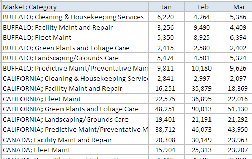
Figure 6-6: Matrix-style reports are often problematic in PivotTables.
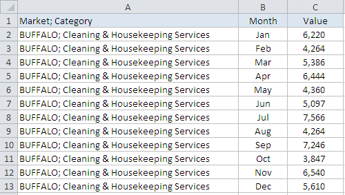
Figure 6-7: Tabular data sets are ideal when working with data.
There are countless methods you can use to transpose an entire data range. The macro in this section provides an easy way to automate this task.
Multiple consolidation ranges can only output three base fields: Row, Column, and Value. The Row field is always made up of the first column in your data source. The Column field is made up of all the column headers after the first column in your data source. The Value field is made up of the values in your data source.
Because of this, you can only have one dimension column. To understand this, take a look at Figure 6-6. Note that the first column is essentially a concatenated column consisting of two data dimensions: Market and Category. This is because a multiple consolidation range pivot table can handle only one dimension field.
How it works
You can transpose a dataset with a multiple consolidation range PivotTable. The manual steps to do so are
1. Press Alt+D+P to call up the Excel 2003 PivotTable Wizard.
2. Click the option for Multiple Consolidation Ranges, and then click Next.
3. Select the I Will Create the Page Fields option, and then click Next.
4. Define the range you are working with and click Finish to create the PivotTable.
5. Double-click on the intersection of the Grand Total row and column.
This macro duplicates the steps above, allowing you to transpose your data set in a fraction of the time.
Sub Macro77()
‘Step 1: Declare your Variables
Dim SourceRange As Range
Dim GrandRowRange As Range
Dim GrandColumnRange As Range
‘Step 2: Define your data source range
Set SourceRange = Sheets(“Sheet1”).Range(“A4:M87”)
‘Step 3: Build Multiple Consolidation Range Pivot Table
ActiveWorkbook.PivotCaches.Create(SourceType:=xlConsolidation, _
SourceData:=SourceRange.Address(ReferenceStyle:=xlR1C1), _
Version:=xlPivotTableVersion14).CreatePivotTable _
TableDestination:=””, _
TableName:=”Pvt2”, _
DefaultVersion:=xlPivotTableVersion14
‘Step 4: Find the Column and Row Grand Totals
ActiveSheet.PivotTables(1).PivotSelect “'Row Grand Total'”
Set GrandRowRange = Range(Selection.Address)
ActiveSheet.PivotTables(1).PivotSelect “'Column Grand Total'”
Set GrandColumnRange = Range(Selection.Address)
‘Step 5: Drill into the intersection of Row and Column
Intersect(GrandRowRange, GrandColumnRange).ShowDetail = True
End Sub
How to use it
You can implement this kind of a macro in a standard module:
1. Activate the Visual Basic Editor by pressing ALT+F11.
2. Right-click the project/workbook name in the Project window.
3. Choose Insert⇒Module.
4. Type or paste the code.