Chapter 10

Routing Protocols

The Following CompTIA Network+ Exam Objectives Are Covered in This Chapter:

• 1.4 Explain the purpose and properties of routing and switching.
  • EIGRP
  • OSPF
  • RIP
  • Routing metrics
• Hop counts
• MTU, bandwidth
• Costs
• Latency
• Next hop
• Routing tables
• Convergence (steady state)
• 2.1 Given a scenario, install and configure routers and switches.
  • Routing tables

Routing protocols are critical to a network’s design. This chapter focuses on dynamic routing protocols. Dynamic routing protocols run only on routers that use them in order to discover networks and update their routing tables. Using dynamic routing is easier on you, the system administrator, than using the labor-intensive, manually achieved, static routing method, but it’ll cost you in terms of router CPU processes and bandwidth on the network links.

The source of the increased bandwidth usage and CPU cycles is the operation of the dynamic routing protocol itself. A router running a dynamic routing protocol shares routing information with its neighboring routers, and it requires additional CPU cycles and additional bandwidth to accomplish that.

In this chapter, I’ll give you all the basic information you need to know about routing protocols so you can choose the correct one for each network you work on or design.

Routing Protocol Basics

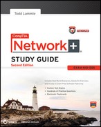
Because getting a solid visual can really help people learn, I’ll get you started by combining the last few figures used in Chapter 9, “Introduction to IP Routing.” This way, you can get the big picture and really understand how routing works. Figure 10-1 shows the complete routing tree that I broke up piece by piece at the end of Chapter 9.

As I touched on in Chapter 9, two types of routing protocols are used in internetworks: interior gateway protocols (IGPs) and exterior gateway protocols (EGPs). IGPs are used to exchange routing information with routers in the same autonomous system (AS). An AS is a collection of networks under a common administrative domain, which simply means that all routers sharing the same routing table information are in the same AS. EGPs are used to communicate between multiple ASs. A nice example of an EGP would be Border Gateway Protocol (BGP), which really is beyond the scope of this book; I’ll briefly describe it in this chapter anyway because there is a small objective about it on the exam. And no worries, we’ll continue our discussion of IGPs too.

There are a few key points about routing protocols that I think it would be a good idea to talk over before getting deeper into the specifics of each one. First on the list is something known as an administrative distance.

Administrative Distances

The administrative distance (AD) is used to rate the trustworthiness of routing information received on one router from its neighboring router. An AD is an integer from 0 to 255, where 0 equals the most trusted route and 255 the least. A value of 255 essentially means, “No traffic is allowed to be passed via this route.”

If a router receives two updates listing the same remote network, the first thing the router checks is the AD. If one of the advertised routes has a lower AD than the other, the route with the lower AD is the one that will get placed in the routing table.

If both advertised routes to the same network have the same AD, then routing protocol metrics like hop count or the amount of bandwidth on the lines will be used to find the best path to the remote network. And as it was with the AD, the advertised route with the lowest metric will be placed in the routing table. But if both advertised routes have the same AD as well as the same metrics, then the routing protocol will load-balance to the remote network. To perform load balancing, a router will send packets down each link to test for the best one.

Table 10-1 shows the default ADs that a router uses to decide which route to take to a remote network.

Table 10-1: Default administrative distances

Route source	Default AD
Connected interface	0
Static route	1
EIGRP	90
IGRP	100
OSPF	110
RIP	120
External EIGRP	170
Unknown	255 (this route will never be used)

Understand that if a network is directly connected, the router will always use the interface connected to that network. Also good to know is that if you configure a static route, the router will believe that route to be the preferred one over any other routes it learns about dynamically. You can change the ADs of static routes, but by default, they have an AD of 1. That’s only one place above zero, so you can see why a static route’s default AD will always be considered the best by the router.

This means that if you have a static route, a RIP-advertised route, and an EIGRP-advertised route listing the same network, then by default, the router will always use the static route unless you change the AD of the static route.

Classes of Routing Protocols

The three classes of routing protocols introduced in Chapter 9, and shown in Figure 10-1, are as follows:

Distance vector The distance vector protocols find the best path to a remote network by judging—you guessed it—distance. Each time a packet goes through a router, it equals something we call a hop. The route with the fewest hops to the network is determined to be the best route. The vector indicates the direction to the remote network. RIP, RIPv2, and Interior Gateway Routing Protocol (IGRP) are distance vector routing protocols. These protocols send the entire routing table to all directly connected neighbors.

Link State Using link state protocols, also called shortest path first protocols, the routers each create three separate tables. One of these tables keeps track of directly attached neighbors, one determines the topology of the entire internetwork, and one is used as the actual routing table. Link state routers know more about the internetwork than any distance vector routing protocol. OSPF and IS-IS are IP routing protocols that are completely link state. Link state protocols send updates containing the state of their own links to all other routers on the network.

Hybrid A hybrid protocol uses aspects of both distance vector and link state, and at this writing, there’s only one—EIGRP. It happens to be a Cisco-proprietary protocol, meaning that it will run on only Cisco equipment. So if you have a multivendor environment, by default, this won’t work for you.

I want you to understand that there’s no one set way of configuring routing protocols for use in every situation. This is something you really have to do on a case-by-case basis. Even though this might seem a little intimidating, if you understand how each of the different routing protocols works, I promise you’ll be capable of making good, solid decisions that will truly meet the individual needs of any business!

Distance Vector Routing Protocols

Okay, the distance vector routing algorithm passes complete routing table contents to neighboring routers, which then combine the received routing table entries with their own routing tables to complete the router’s routing table. This is called routing by rumor because a router receiving an update from a neighbor router believes the information about remote networks without finding out for itself if it actually is correct.

It’s possible to have a network that has multiple links to the same remote network, and if that’s the case, the AD of each received update is checked first. As I said, if the AD is the same, the protocol will then have to use other metrics to determine the best path to use to get to that remote network.

Distance vector uses only hop count to determine the best path to a network. If a router finds more than one link with the same hop count to the same remote network, it will automatically perform what’s known as round-robin load balancing.

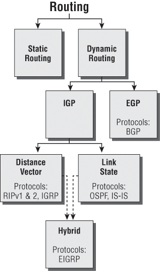
It’s important to understand what a distance vector routing protocol does when it starts up. In Figure 10-2, the four routers start off with only their directly connected networks in their routing table. After a distance vector routing protocol is started on each router, the routing tables are then updated with all route information gathered from neighbor routers.

As you can see in Figure 10-2, each router has only the directly connected networks in each of its routing tables. Each router sends its complete routing table, which includes the network number, exit interface, and hop count to the network, out to each active interface.

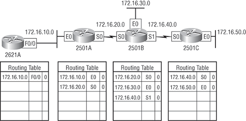
Now, in Figure 10-3, the routing tables are complete because they include information about all the networks in the internetwork. They are considered converged. Usually, data transmission will cease while routers are converging—a good reason in favor of fast convergence time! In fact, one of the main problems with RIP is its slow convergence time.

As you can see in Figure 10-3, once all the routers have converged, the routing table in each router keeps information about three important things:

• The remote network number
• The interface that the router will use to send packets to reach that particular network
• The hop count, or metric, to the network

Let’s start discussing dynamic routing protocols with one of the oldest routing protocols that is still in existence today.

Routing Information Protocol (RIP)

RIP is a true distance vector routing protocol. It sends the complete routing table out to all active interfaces every 30 seconds. RIP uses only one thing to determine the best way to a remote network—the hop count. And because it has a maximum allowable hop count of 15 by default, a hop count of 16 would be deemed unreachable. This means that although RIP works fairly well in small networks, it’s pretty inefficient on large networks with slow WAN links or on networks populated with a large number of routers.

RIP version 1 uses only classful routing, which means that all devices in the network must use the same subnet mask. This is because RIP version 1 doesn’t send updates with subnet mask information in tow. RIP version 2 provides something called prefix routing and does send subnet mask information with the route updates. Doing this is called classless routing.

RIP Version 2 (RIPv2)

Let’s spend a couple of minutes discussing RIPv2 before we move into the advanced distance vector (also referred to as hybrid), Cisco-proprietary routing protocol EIGRP.

RIP version 2 is mostly the same as RIP version 1. Both RIPv1 and RIPv2 are distance vector protocols, which means that each router running RIP sends its complete routing tables out all active interfaces at periodic time intervals. Also, the timers and loop-avoidance schemes are the same in both RIP versions. Both RIPv1 and RIPv2 are configured with classful addressing (but RIPv2 is considered classless because subnet information is sent with each route update), and both have the same AD (120).

But there are some important differences that make RIPv2 more scalable than RIPv1. And I’ve got to add a word of advice here before we move on: I’m definitely not advocating using RIP of either version in your network. But because RIP is an open standard, you can use RIP with any brand of router. You can also use OSPF because OSPF is an open standard as well.

Table 10-2 discusses the differences between RIPv1 and RIPv2.

Table 10-2: RIPv1 vs. RIPv2

RIPv1	RIPv2
Distance vector	Distance vector
Maximum hop count of 15	Maximum hop count of 15
Classful	Classless
Broadcast based	Uses multicast 224.0.0.9
No support for VLSM	Supports VLSM networks
No authentication	Allows for MD5 authentication
No support for discontiguous networks	Supports discontiguous networks (covered in the next section)

RIPv2, unlike RIPv1, is a classless routing protocol (even though it is configured as classful, like RIPv1), which means that it sends subnet mask information along with the route updates. By sending the subnet mask information with the updates, RIPv2 can support Variable Length Subnet Masks (VLSMs), which are described in the next next section; in addition, network boundaries are summarized.

VLSM and Discontiguous Networks

VLSM allows classless routing, meaning that the routing protocol sends subnet-mask information with the route updates. The reason it’s good to do this is to save address space. If we didn’t use a routing protocol that supports VLSMs, then every router interface, every node (PC, printer, server, and so on), would have to use the same subnet mask.

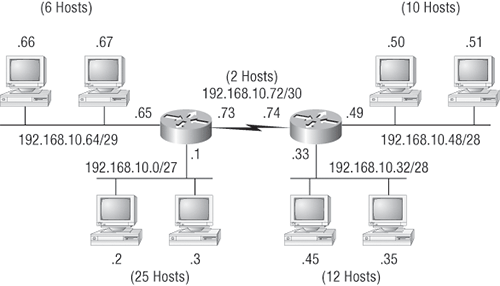
As the name suggests, with VLSMs we can have different subnet masks for different router interfaces. Check out Figure 10-4 to see an example of why classful network designs are inefficient.

Looking at this figure, you’ll notice that we have two routers, each with two LANs and connected together with a WAN serial link. In a typical classful network design example (RIP or RIPv2 routing protocol), you could subnet a network like this:

192.168.10.0 = Network

255.255.255.240 (/28) = Mask

Our subnets would be (you know this part, right?) 0, 16, 32, 48, 64, 80, and so on. This allows us to assign 16 subnets to our internetwork. But how many hosts would be available on each network? Well, as you probably know by now, each subnet provides only 14 hosts. This means that with a /28 mask each LAN can support 14 valid hosts—one LAN requires 25 addresses, so a /28 mask doesn’t provide enough addresses for the hosts in that LAN! Moreover the point-to-point WAN link also would consume 14 addresses when only two are required. It’s too bad we can’t just nick some valid hosts from that WAN link and give them to our LANs.

All hosts and router interfaces have the same subnet mask—again, this is called classful routing. And if we want this network to be more efficient, we definitely need to add different masks to each router interface.

But there’s still another problem—the link between the two routers will never use more than two valid hosts! This wastes valuable IP address space, and it’s the big reason I’m talking to you about VLSM networking.

Now let’s take Figure 10-4 and use a classless design…which will become the new network shown in Figure 10-5. In the previous example, we wasted address space—one LAN didn’t have enough addresses because every router interface and host used the same subnet mask. Not so good.

What would be good is to provide only the needed number of hosts on each router interface, meaning VLSMs.

So, if we use a /30 on our WAN links and a /27, /28, and /29 on our LANs, we’ll get 2 hosts per WAN interface and 30, 14, and 6 hosts per LAN interface—nice! This makes a huge difference—not only can we get just the right number of hosts on each LAN, we still have room to add more WANs and LANs using this same network.

Remember, in order to implement a VLSM design on your network, you need to have a routing protocol that sends subnet-mask information with the route updates. This would be RIPv2, EIGRP, or OSPF. RIPv1 and IGRP will not work in classless networks and are considered classful routing protocols.

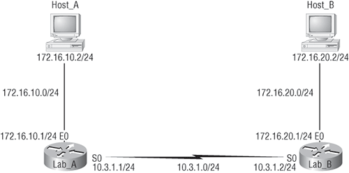
Now, what’s a discontiguous network? It’s one that has two or more subnetworks of a classful network connected together by different classful networks. Figure 10-6 displays a typical discontiguous network.

The subnets 172.16.10.0 and 172.16.20.0 are connected together with a 10.3.1.0 network. By default, each router thinks it has the only 172.16.0.0 classful network.

It’s important to understand that discontiguous networks just won’t work with RIPv1 at all. They don’t work by default on RIPv2 or EIGRP either, but discontiguous networks do work on OSPF networks by default because OSPF does not auto-summarize like RIPv2 and EIGRP.

EIGRP

EIGRP is a classless, Cisco proprietary, enhanced distance-vector protocol that possesses a real edge over another Cisco proprietary protocol, IGRP. That’s basically why it’s called Enhanced IGRP.

EIGRP uses the concept of an autonomous system to describe the set of contiguous routers that run the same routing protocol and share routing information. But unlike IGRP, EIGRP includes the subnet mask in its route updates. And as you now know, the advertisement of subnet information allows us to use VLSMs when designing our networks.

EIGRP is referred to as a hybrid routing protocol because it has characteristics of both distance vector and link state protocols. For example, EIGRP doesn’t send link state packets as OSPF does; instead, it sends traditional distance vector updates containing information about networks plus the cost of reaching them from the perspective of the advertising router. But EIGRP has link state characteristics as well—it synchronizes routing tables between neighbors at startup and then sends specific updates only when topology changes occur. This makes EIGRP suitable for very large networks.

There are a number of powerful features that make EIGRP a real standout from RIP, RIPv2, and other protocols. The main ones are listed here:

• Support for IP and IPv6 (and some other useless routed protocols) via protocol-dependent modules
• Considered classless (same as RIPv2 and OSPF)
• Support for VLSM / Classless Inter-Domain Routing (CIDR)
• Support for summaries and discontiguous networks
• Efficient neighbor discovery
• Communication via Reliable Transport Protocol (RTP)
• Best path selection via Diffusing Update Algorithm (DUAL)

Another great feature of EIGRP is that it’s simple to configure and turn on like a distance vector protocol, but it keeps track of more information than distance vector does. It creates and maintains additional tables instead of just one table as distance vector routing protocols do.

These tables are called the neighbor table, topology table, and routing table, as shown in Figure 10-7.

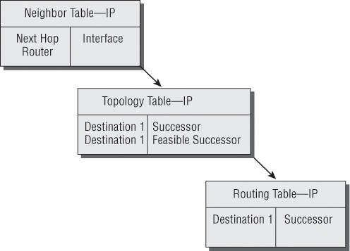
Neighbor table Each router keeps state information about adjacent neighbors. When a newly discovered neighbor is learned on a router interface, the address and interface of that neighbor are recorded, and the information is held in the neighbor table and stored in RAM. Sequence numbers are used to match acknowledgments with update packets. The last sequence number received from the neighbor is recorded so that out-of-order packets can be detected.

Topology table The topology table is populated by the neighbor table, and the best path to each remote network is found by running Diffusing Update Algorithm (DUAL). The topology table contains all destinations advertised by neighboring routers, holding each destination address and a list of neighbors that have advertised the destination. For each neighbor, the advertised metric, which comes only from the neighbor’s routing table, is recorded. If the neighbor is advertising this destination, it must be using the route to forward packets.

Feasible successor (backup routes) A feasible successor is a path whose reported distance is less than the feasible (best) distance, and it is considered a backup route. EIGRP will keep up to six feasible successors in the topology table. Only the one with the best metric (the successor) is copied and placed in the routing table.

Successor (routes in a routing table) A successor route (think successful!) is the best route to a remote network. A successor route is used by EIGRP to forward traffic to a destination and is stored in the routing table. It is backed up by a feasible successor route that is stored in the topology table—if one is available.

By using the feasible distance and having feasible successors in the topology table as backup links, EIGRP allows the network to converge instantly and updates to any neighbor only consist of traffic sent from EIGRP. All of these things make for a very fast, scalable, fault-tolerant routing protocol.

Border Gateway Protocol (BGP)

In a way, you can think of Border Gateway Protocol (BGP) as the heavyweight of routing protocols. This is an external routing protocol (used between autonomous systems, unlike RIP or OSPF, which are internal routing protocols) that uses a sophisticated algorithm to determine the best route. In fact, it just happens to be the core routing protocol of the Internet. And it’s not exactly breaking news that the Internet has become a vital resource in so many organizations, is it? No—but this growing dependence has resulted in redundant connections to many different ISPs.

This is where BGP comes in. The sheer onslaught of multiple connections would totally overwhelm other routing protocols like OSPF, which I am going to talk about in the next section. BGP is essentially an alternative to using default routes for controlling path selections. Default routes are configured on routers to control packets that have a destination IP address that is not found in the routing table. Please see CCNA: Cisco Certified Network Associate Study Guide (Sybex, 2011) for more information on static and default routing.

Because the Internet’s growth rate shows no signs of slowing, ISPs use BGP for its ability to make classless routing and summarization possible. These capabilities help to keep routing tables smaller and more efficient at the ISP core.

BGP is used for IGPs to communicate ASs together in larger networks, if needed, as shown in Figure 10-8.

So yes, very large private IP networks can make use of BGP. Let’s say you wanted to join a number of large OSPF networks together. Because OSPF just couldn’t scale up enough to handle such a huge load, you would go with BGP instead to connect the ASs together. Another situation in which BGP would come in really handy would be if you wanted to multi-home a network for better redundancy, either to a multiple access point of a single ISP or to multiple ISPs.

Internal routing protocols are employed to advertise all available networks, including the metric necessary to get to each of them. BGP is a personal favorite of mine because its routers exchange path vectors that give you detailed information on the BGP AS numbers, hop by hop (called an AS-Path), required to reach a specific destination network.

And BGP also tells you about any/all networks reachable at the end of the path. These factors are the biggest differences you need to remember about BGP. Unlike IGPs that simply tell you how to get to a specific network, BGP gives you the big picture on exactly what’s involved in getting to an AS, including the networks located in that AS itself.

And there’s more to that “BGP big picture”—this protocol carries information like the network prefixes found in the AS and includes the IP address needed to get to the next AS, (the next-hop attribute). It even gives you the history on how the networks at the end of the path were introduced into BGP in the first place, known as the origin code attribute.

All of these traits are what makes BGP so useful for constructing a graph of loop-free autonomous systems, for identifying routing policies, and for enabling us to create and enforce restrictions on routing behavior based upon the AS path—sweet!

Link State Routing Protocols

Link state protocols also fall into the classless category of routing protocols, and they work within packet-switched networks. OSPF and IS-IS are two examples of link state routing protocols.

Remember, for a protocol to be a classless routing protocol, the subnet-mask information must be carried with the routing update so that all neighbor routers know the cost of the network route that’s being advertised. One of the biggest differences between link state and distance vector protocols is that link state protocols learn and maintain much more information about the internetwork than distance vector routing protocols do. Distance vector routing protocols maintain only a routing table with the destination routes in it. Link state routing protocols maintain two additional tables with more detailed information, with the first of these being the neighbor table. The neighbor table is maintained through the use of hello packets that are exchanged by all routers to determine which other routers are available to exchange routing data with. All routers that can share routing data are stored in the neighbor table.

The second table maintained is the topology table, which is built and sustained through the use of link state advertisements or packets (LSAs or LSPs, depending on the protocol). In the topology table, you’ll find a listing for every destination network plus every neighbor (route) through which it can be reached. Essentially, it’s a map of the entire internetwork.

Once all of that raw data is shared and each one of the routers has the data in its topology table, the routing protocol runs the Shortest Path First (SPF) algorithm to compare it all and determine the best paths to each of the destination networks.

Open Shortest Path First (OSPF)

Open Shortest Path First (OSPF) is an open-standard routing protocol that’s been implemented by a wide variety of network vendors, including Cisco. OSPF works by using the Dijkstra algorithm. First, a shortest-path tree is constructed, and then the routing table is populated with the resulting best paths. OSPF converges quickly (although not as fast as EIGRP), and it supports multiple, equal-cost routes to the same destination. Like EIGRP, it supports both IP and IPv6 routed protocols, but OSPF must maintain a separate database and routing table for each, meaning you’re basically running two routing protocols if you are using IP and IPv6 with OSPF.

OSPF provides the following features:

• Consists of areas and autonomous systems
• Minimizes routing update traffic
• Allows scalability
• Supports VLSM/CIDR
• Has unlimited hop count
• Allows multivendor deployment (open standard)

OSPF is the first link state routing protocol that most people are introduced to, so it’s good to see how it compares to more traditional distance vector protocols like RIPv2 and RIPv1. Table 10-3 gives you a comparison of these three protocols.

Table 10-3: OSPF and RIP comparison

OSPF has many features beyond the few I’ve listed in Table 10-3, and all of them contribute to a fast, scalable, and robust protocol that can be actively deployed in thousands of production networks. One of the most noteworthy of its features is that after a network change (link up or down), OSPF converges (convergence is when all routers have been updated with the change) of any of the interior routing protocols we will discuss.

OSPF is supposed to be designed in a hierarchical fashion, which basically means that you can separate the larger internetwork into smaller internetworks called areas. This is definitely the best design for OSPF.

The following are reasons you really want to create OSPF in a hierarchical design:

• To decrease routing overhead
• To speed up convergence
• To confine network instability to single areas of the network

Pretty sweet benefits! But you have to earn them—OSPF is more elaborate and difficult to configure in this manner.

Figure 10-9 shows a typical OSPF simple design. Notice how each router connects to the backbone—called area 0, or the backbone area. OSPF must have an area 0, and all other areas should connect to this area. Routers that connect other areas to the backbone area within an AS are called area border routers (ABRs). Still, at least one interface of the ABR must be in area 0.

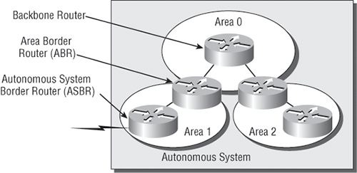
OSPF runs inside an autonomous system, but it can also connect multiple autonomous systems together. The router that connects these ASs is called an autonomous system border router (ASBR). Typically, in today’s networks, BGP is used to connect between ASs, not OSPF.

Ideally, you would create other areas of networks to help keep route updates to a minimum and to keep problems from propagating throughout the network. But that’s beyond the scope of this chapter. Just make note of it for your future networking studies.

Intermediate System-to-Intermediate System (IS-IS)

IS-IS is an IGP, meaning that it’s intended for use within an administrative domain or network, not for routing between ASs. That would be a job that an EGP (such as BGP, which we just covered) would handle instead.

IS-IS is a link state routing protocol, meaning it operates by reliably flooding topology information throughout a network of routers. Each router then independently builds a picture of the network’s topology, just as OSPF does. Packets or datagrams are forwarded based on the best topological path through the network to the destination.

Figure 10-10 shows an IS-IS network and the terminology used with IS-IS.

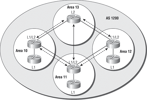
Here are the definitions for the terms used in the IS-IS network shown in Figure 10-10:

L1 Level 1 intermediate systems route within an area. When the destination is outside an area, they route toward a Level 2 system.

L2 Level 2 intermediate systems route between areas and toward other ASs.

The difference between IS-IS and OSPF is that IS-IS uses Connectionless Network Service (CLNS) to provide connectionless delivery of data packets between routers. OSPF uses IP to communicate between routers instead.

An advantage to having CLNS around is that it can easily send information about multiple routed protocols (IP and IPv6), and as I already mentioned, OSPF must maintain a completely different routing database for IP and IPv6, respectively, for it to be able to send updates for both protocols.

IS-IS supports the most important characteristics of OSPF and EIGRP because it supports VLSM and also because it converges quickly. Each of these three protocols has advantages and disadvantages, but it’s these two shared features that make any of them scalable and appropriate for supporting the large-scale networks of today.

One last thing—even though it’s not as common, IS-IS, although comparable to OSPF, is actually preferred by ISPs because of its ability to run IP and IPv6 without creating a separate database for each protocol as OSPF does. That single feature makes it more efficient in very large networks.

IPv6 Routing Protocols

Most of the routing protocols we’ve already discussed have been upgraded for use in IPv6 networks. Also, many of the functions and configurations that we’ve already learned will be used in almost the same way as they’re used now. Knowing that broadcasts have been eliminated in IPv6, it follows that any protocols that use entirely broadcast traffic will go the way of the dodo—but unlike the dodo, it’ll be good to say goodbye to these bandwidth-hogging, performance-annihilating little gremlins!

The routing protocols that we’ll still use in version 6 got a new name and a facelift. Let’s talk about a few of them now.

First on the list is RIPng (next generation). Those of you who have been in IT for a while know that RIP has worked very well for us on smaller networks, which happens to be the reason it didn’t get whacked and will still be around in IPv6. And we still have EIGRPv6 because it already had protocol-dependent modules and all we had to do was add a new one to it for the IPv6 protocol. Rounding out our group of protocol survivors is OSPFv3—that’s not a typo, it really is version 3. OSPF for IPv4 was actually version 2, so when it got its upgrade to IPv6, it became OSPFv3.

RIPng

To be honest, the primary features of RIPng are the same as they were with RIPv2. It is still a distance vector protocol, has a max hop count of 15, and still has the same loop avoidance mechanisms as well as using UDP port 521.

And it still uses multicast to send its updates too, but in IPv6, it uses FF02::9 for the transport address. This is actually kind of cool because in RIPv2, the multicast address was 224.0.0.9, so the address still has a 9 at the end in the new IPv6 multicast range. In fact, most routing protocols got to keep a little bit of their IPv4 identities like that.

But of course there are differences in the new version or it wouldn’t be a new version, would it? We know that routers keep the next-hop addresses of their neighbor routers for every destination network in their routing table. The difference is that with RIPng, the router keeps track of this next-hop address using the link-local address, not a global address. So just remember that RIPng will pretty much work the same way as with IPv4.

EIGRPv6

As with RIPng, EIGRPv6 works much the same as its IPv4 predecessor does—most of the features that EIGRP provided before EIGRPv6 will still be available.

EIGRPv6 is still an advanced distance vector protocol that has some link state features. The neighbor-discovery process using hellos still happens, and it still provides reliable communication with a reliable transport protocol that gives us loop-free fast convergence using DUAL.

Hello packets and updates are sent using multicast transmission, and as with RIPng, EIGRPv6’s multicast address stayed almost the same. In IPv4 it was 224.0.0.10; in IPv6, it’s FF02::A (A = 10 in hexadecimal notation).

Last to check out in our group is what OSPF looks like in the IPv6 routing protocol.

OSPFv3

The new version of OSPF continues the trend of the routing protocols having many similarities with their IPv4 versions.

The foundation of OSPF remains the same—it is still a link state routing protocol that divides an entire internetwork or autonomous system into areas, making a hierarchy.

Adjacencies (neighbor routers running OSPF) and next-hop attributes now use link-local addresses, and OSPFv3 still uses multicast traffic to send its updates and acknowledgements, with the addresses FF02::5 for OSPF routers and FF02::6 for OSPF-designated routers, which provide topological updates (route information) to other routers. These new addresses are the replacements for 224.0.0.5 and 224.0.0.6, respectively, which were used in OSPFv2.

With all this routing information behind you, it’s time to go through some review questions and then move on to learning all about switching in the next chapter.

Summary

This chapter covered the basic routing protocols that you may find on a network today. Probably the most common routing protocols you’ll run into are RIP, OSPF, and EIGRP.

I covered RIP, RIPv2, the differences between the two RIP protocols, EIGRP, and BGP in the section on distance vector protocols.

I finished by discussing OSPF and IS-IS and when you would possibly see each one in a network.

Exam Essentials

Remember the differences between RIPv1 and RIPv2. RIPv1 sends broadcasts every 30 seconds and has an AD of 120. RIPv2 sends multicasts (224.0.0.9) every 30 seconds and also has an AD of 120. RIPv2 sends subnet mask information with the route updates, which allows it to support classless networks and discontiguous networks. RIPv2 also supports authentication between routers, and RIPv1 does not.

Know EIGRP features. EIGRP is a classless, advanced distance vector protocol that supports IP, IPX, AppleTalk, and now IPv6. EIGRP uses a unique algorithm called DUAL to maintain route information, and it uses RTP to communicate with other EIGRP routers reliably.

Compare OSPF and RIPv1. OSPF is a link state protocol that supports VLSM and classless routing; RIPv1 is a distance vector protocol that does not support VLSM and supports only classful routing.

Written Lab

1. The default administrative distance of RIP is___________________.

2. The default administrative distance of EIGRP is___________________.

3. The default administrative distance of RIPv2 is___________________.

4. What is the default administrative distance of a static route?

5. What is the version or name of RIP that is used with IPv6?

6. What is the version or name of OSPF that is used with IPv6?

7. What is the version or name of EIGRP that is used with IPv6?

8. When would you use BGP?

9. When could you use EIGRP?

10. Is BGP considered link state or distance vector?

You can find the answers in Appendix B.

Review Questions

You can find the answers in Appendix A.

1. Which of the following protocols support VLSM, summarization, and discontiguous networking? (Choose three.)

A. RIPv1

B. IGRP

C. EIGRP

D. OSPF

E. BGP

F. RIPv2

2. Which of the following are considered distance vector routing protocols? (Choose two.)

A. OSPF

B. RIP

C. RIPv2

D. IS-IS

3. Which of the following are considered link state routing protocols? (Choose two.)

A. OSPF

B. RIP

C. RIPv2

D. IS-IS

4. Which of the following is considered a hybrid routing protocol?

A. OSPF

B. BGP

C. RIPv2

D. IS-IS

E. EIGRP

5. Why would you want to use a dynamic routing protocol instead of using static routes?

A. There is less overhead on the router.

B. Dynamic routing is more secure.

C. Dynamic routing scales to larger networks.

D. The network runs faster.

6. Which of the following is a vendor-specific routing protocol?

A. STP

B. OSPF

C. RIPv1

D. EIGRP

E. IS-IS

7. RIP has a long convergence time and users have been complaining of response time when a router goes down and RIP has to reconverge. Which can you implement to improve convergence time on the network?

A. Replace RIP with static routes.

B. Update RIP to RIPv2.

C. Update RIP to OSPF using link state.

D. Replace RIP with BGP as an exterior gateway protocol.

8. What is the administrative distance of OSPF?

A. 90

B. 100

C. 110

D. 120

9. Which of the following protocols will advertise routed IPv6 networks?

A. RIP

B. RIPng

C. OSPFv2

D. EIGRPv3

10. What is the difference between static and dynamic routing?

A. You use static routing in large, scalable networks.

B. Dynamic routing is used by a DNS server.

C. Dynamic routes are added automatically.

D. Static routes are added automatically.

11. Which routing protocol has a maximum hop count of 15?

A. RIPv1

B. IGRP

C. EIGRP

D. OSPF

12. Which of the following describes routing convergence time?

A. The time it takes for your VPN to connect

B. The time required by protocols to update their forwarding tables after changes have occurred

C. The time required for IDS to detect an attack

D. The time required by switches to update their link status and go into forwarding state

13. What routing protocol is typically used to connect ASs on the Internet?

A. IGRP

B. RIPv2

C. BGP

D. OSPF

14. RIPv2 sends out its routing table every 30 seconds just like RIPv1, but it does so more efficiently. What type of transmission does RIPv2 use to accomplish this task?

A. Broadcasts

B. Multicasts

C. Telecast

D. None of the above

15. Which routing protocols have an administrative distance of 120? (Choose two.)

A. RIPv1

B. RIPv2

C. EIGRP

D. OSPF

16. Which of the following routing protocols uses AS-Path as one of the methods to build the routing tables?

A. OSPF

B. IS-IS

C. BGP

D. RIP

E. EIGRP

17. Which IPv6 routing protocol uses UDP port 521?

A. RIPng

B. EIGRPv6

C. OSPFv3

D. IS-IS

18. What EIGRP information is held in RAM and maintained through the usage of hello and update packets? (Select all that apply.)

A. DUAL table

B. Neighbor table

C. Topology table

D. Successor route

19. Which is true regarding EIGRP successor routes?

A. Successor routes are saved in the neighbor table.

B. Successor routes are stored in the DUAL table.

C. Successor routes are used only if the primary route fails.

D. A successor route is used by EIGRP to forward traffic to a destination.

20. Which of the following uses only hop count as a metric to find the best path to a remote network?

A. RIP

B. EIGRP

C. OSPF

D. BGP