Chapter 13
Performance Tuning T-SQL
WHAT’S IN THIS CHAPTER
- Query Processing Including Tools Usage and Optimization
- The Query Tuning Process Including Joins, Query Plans, and Indexes
Performance tuning T-SQL is interesting but also quite frequently frustrating. It is interesting because there is so much involved in tuning that knowledge of SQL Server’s architecture and internals plays a large role in doing it well. It can be frustrating when you do not have access to change the source query as it resides inside a vendor application, or when it seems that whatever optimization technique is tried, the performance issue does not seem to be resolved. Of course, knowledge alone is not sufficient without the right tools, which you learn about in this chapter. If you have tuned a query and reduced its runtime, you may have jumped up and down with excitement, but sometimes you cannot achieve that result even after losing sleep for many nights.
In this chapter, you learn how to gather the data for query tuning, the tools for query tuning, the stages a query goes through before execution, and a little bit on how to analyze the execution plan. You must understand which stages a query passes through before actually being executed by the execution engine, so start with physical query processing.
PHYSICAL QUERY PROCESSING PART ONE: COMPILATION AND RECOMPILATION
SQL Server performs two main steps to produce the desired result when a query fires. As you would guess, the first step is query compilation, which generates the query plan; the second step is the execution of the query plan (this will be discussed later in the chapter). The compilation phase in SQL Server 2012 goes through three steps: parsing, algebrization, and optimization. In SQL Server 2000, there was a normalization phase, which was replaced with the algebrization piece in SQL Server 2005. The SQL Server team has spent much effort to re-architect and rewrite several parts of SQL Server. Of course, the goal is to redesign logic to serve current and future expansions of SQL Server functionality. Having said that, after the three steps just mentioned are completed, the compiler stores the optimized query plan in the plan cache.
Now you are going to investigate compilation and recompilation of queries, with a detailed look at parsing, algebrization and optimization in detail.
Compilation
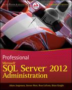
Before a query, batch, stored procedure, trigger, or dynamic SQL statement begins execution on SQL Server 2012, the batch is compiled into a plan. The plan is then executed for its effects or to produce results. The flowchart in Figure 13-1 displays the steps in the compilation process in SQL Server 2012.
When a batch starts, the compilation process tries to find the cached plan in the plan cache. If it finds a match, the execution engine takes over. If a match is not found, the parser starts parsing (explained later in this section). The plan guide match feature (introduced with SQL Server 2005) determines whether an existing plan guide for a particular statement exists. (You learn how to create the plan guide later.) If it exists, it uses the plan guide for that statement for execution. (The concepts of forced autoparam and simple autoparam are described later in the chapter.) If a match is found, the plan is sent to the algebrizer (explained later in this section), which creates a logical, or parse, tree for input to the optimizer (also explained later in this section). The logical tree or parse tree is generated by the process that checks whether the T-SQL is written correctly. The parse tree represents the logical steps necessary to execute the query. The plan is then cached in the plan cache. Of course, not all the plans are cached; for example, when you create a stored procedure with WITH RECOMPILE, the plan is not cached.
Recompilation
Sometimes a cached plan needs to be recompiled because it is not valid for some reason. Suppose that a batch has been compiled into a collection of one or more query plans. SQL Server 2012 checks for validity (correctness) and optimality of that query plan before it begins executing any of the individual query plans. If one of the checks fails, the statement corresponding to the query plan or the entire batch is compiled again, and a possibly different query plan is produced. Such compilations are known as recompilations.
From SQL Server 2005 onward, if a statement in a batch causes the recompilation, then only that statement recompiles, not the whole batch. This statement-level recompilation has some advantages. In particular, it results in less CPU time and memory use during batch recompilations and obtains fewer compile locks. Prior to this change, if you had a long stored procedure, it was sometimes necessary to break it into small chunks just to reduce compile time.
The reasons for recompilation can be broadly classified in two categories:
- Correctness
- Plan optimality
Correctness
If the query processor decides that the cache plan would produce incorrect results, it recompiles that statement or batch. There are multiple reasons why the plan would produce incorrect results — changes to the table or view referenced by the query, changes to the indexes used by the execution plan, updates to the statistics, an explicit call to sp_recompile, or executing a stored procedure using the WITH RECOMPILE option. The following sections investigate how the changes that can occur to the schemas of objects cause recompilation as well as how SET options can cause recompilation.
Schemas of Objects
Your query batch could be referencing many objects such as tables, views, user-defined functions (UDFs), or indexes; and if the schemas of any of the objects referenced in the query have changed since your batch was last compiled, your batch must be recompiled for statement-correctness reasons. Schema changes could include many things, such as adding an index on a table or in an indexed view, or adding or dropping a column in a table or view.
Since the release of SQL Server 2005, manually dropping or creating statistics on a table causes recompilation. Recompilation is triggered when the statistics are updated automatically, too. Manually updating statistics does not change the schema version. This means that queries that reference the table but do not use the updated statistics are not recompiled. Only queries that use the updated statistics are recompiled.
Using two-part object names (schema.objectname) is recommended as a best practice. Including the server and database name can cause issues when moving code between servers, for example, from Dev to QA.
Batches with unqualified object names may result in the generation of multiple query plans. For example, in "SELECT * FROM MyTable," MyTable may legitimately resolve to Fred.MyTable if Fred issues this query and he owns a table with that name. Similarly, MyTable may resolve to Joe.MyTable if Joe issues the query. In such cases, SQL Server 2012 does not reuse query plans. If, however, Fred issues "SELECT * FROM dbo.MyTable," and Joe issues the SAME query, there is no ambiguity because the object is uniquely identified, and query plan reuse can happen. However, if Fred runs the query "SELECT * FROM MyTable" a second time, the cached plan will be reused.
SET Options
Some of the SET options affect query results. If the setting of a SET option affecting plan reuse is changed inside of a batch, a compilation happens. The SET options that affect plan reusability are ANSI_NULLS, ANSI_NULL_DFLT_ON, ANSI_PADDING, ANSI_WARNINGS, CURSOR_CLOSE_ON_COMMIT, IMPLICIT_TRANSACTIONS, and QUOTED_IDENTIFIER.
A number of SET options have been marked for deprecation in a future version of SQL Server. The SET options ANSI_NULLS, ANSI_PADDING, and CONCAT_NULLS_YIELDS_NULL will always be set to ON. SET OFFSETS will be unavailable.
These SET options affect plan reuse because SQL Server performs constant folding, evaluating a constant expression at compile time to enable some optimizations, and because the settings of these options affect the results of such expressions.
Listing 13-1 demonstrates how SET options cause recompilation:
LISTING 13-1: RecompileSetOption.sql
USE AdventureWorks
GO

IF OBJECT_ID('dbo.RecompileSetOption') IS NOT NULL
   DROP PROC dbo.RecompileSetOption
GO

CREATE PROC dbo.RecompileSetOption
AS
SET ANSI_NULLS OFF

SELECT s.CustomerID, COUNT(s.SalesOrderID)
FROM Sales.SalesOrderHeader s
GROUP BY s.CustomerID
HAVING COUNT(s.SalesOrderID) > 8
GO

EXEC dbo.RecompileSetOption    -- Causes a recompilation
GO
EXEC dbo.RecompileSetOption    -- does not cause a recompilation
GO
By default, the SET ANSI_NULLS option is ON, so when you compile this stored procedure, it compiles with this option ON. Inside the stored procedure, you have set ANSI_NULLS to OFF, so when you begin executing this stored procedure, the compiled plan is not valid and recompiles with SET ANSI_NULLS OFF. The second execution does not cause a recompilation because the cached plan compiles with "ansi_nulls" set to OFF.
To avoid SET option–related recompilations, establish SET options at connection time, and ensure that they do not change for the duration of the connection. You can do this by not changing set options at any point within a query statement.
Plan Optimality
SQL Server is designed to generate the optimal query execution plan as data changes in your database. As you know, data distributions are tracked with statistics (histograms) for use in the SQL Server query processor. The table content changes because of INSERT, UPDATE, and DELETE operations. Table contents are tracked directly using the number of rows in the table and indirectly using statistics on table columns (explained in detail later in the chapter). The query processor checks the threshold to determine whether it should recompile the query plan, using the following formula:
[ Colmodctr (snapshot) - Colmodctr (current) ] >= RT
Since SQL Server 2005, the table modifications are tracked using Colmodctr. The Colmodctr is stored for each column, so changes to a table can be tracked with finer granularity in SQL Server 2005 and later. Rowmodctr is available in SQL Server 2005 and later, but it is only there for backward compatibility.
In this formula, colmodctr (snapshot) is the value stored at the time the query plan was generated, and colmodctr (current) is the current value. If the difference between these counters as shown in the formula is greater or equal to recompilation threshold (RT), then recompilation happens for that statement. RT is calculated as follows for permanent and temporary tables. The n refers to a table’s cardinality (the number of rows in the table) when a query plan is compiled.
For a permanent table, the formula is as follows:
If n <= 500, RT = 500
If n > 500, RT = 500 + 0.20 * n
For a temporary table, the formula is as follows:
If n < 6, RT = 6
If 6 <= n <= 500, RT = 500
If n > 500, RT = 500 + 0.20 * n
For a table variable, RT does not exist. Therefore, recompilations do not happen because of changes in cardinality to table variables. Table 13-1 shows how the colmodctr is modified in SQL Server 2005 and later through different data manipulation language (DML) statements.
TABLE 13-1: colmodctr Modification
| STATEMENT | COLMODCTR |
| INSERT | All colmodctr + = 1 (colmodctr is incremented by 1 for each column in the table for each insert). |
| DELETE | All colmodctr + = 1 |
| UPDATE | If the update is to non-key columns, colmodctr+= 1 for all of the updated columns. If the update is to key columns, colmodctr+= 2 for all the columns. |
| BULK INSERT | Like n INSERTs. All colmodctr += n (n is the number of rows bulk inserted). |
| TABLE TRUNCATION | Like n DELETEs. All colmodctr += n (n is the table’s cardinal). |
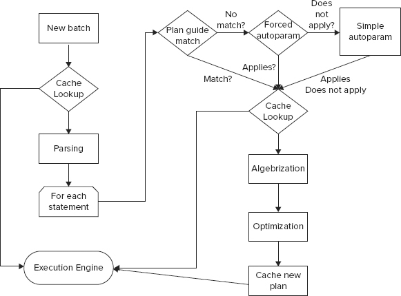
You can see the physical query process in action by following the code in Listing 13-2 and performing the steps associated with it. The goal is to determine whether the stored procedure plan is reused. Listing 13-2 also uses SQL Profiler and the dynamic management view (DMV) sys.dm_exec_cached_plans to examine some interesting details. To determine whether a compiled plan is reused, you must monitor the events SP:CacheMiss, SP:CacheHit, and SP:CacheInsert under the Stored Procedures event class. Figure 13-2 shows these stored procedure plan compilation events in SQL Profiler.
The following steps and code provide a working example of physical query processing.
1. Connect to the SQL Server on which you have the AdventureWorks database.
Don’t do this exercise on a production server!
2. Compile the stored procedure TestCacheReUse in AdventureWorks. The code is as follows in Listing 13-2.
LISTING 13-2: ExecuteSP.sql
USE AdventureWorks
GO
IF OBJECT_ID('dbo.TestCacheReUse') IS NOT NULL
   DROP PROC dbo.TestCacheReUse
GO
CREATE PROC dbo.TestCacheReUse
AS

SELECT BusinessEntityID, LoginID, JobTitle
FROM HumanResources.Employee
WHERE BusinessEntityID = 109
GO
3. Connect the SQL Profiler to your designated machine, and start it after selecting the events (refer to Figure 13-2). Now execute the stored procedure TestCacheReUse as follows:
USE AdventureWorks
GO
EXEC dbo.TestCacheReUse
In SQL Server Profiler you can find the SP:CacheMiss and SP:CacheInsert events, as shown in Figure 13-3.

The SP:CacheMiss event indicates that the compiled plan is not found in the plan cache (refer to Figure 13-3). The stored procedure plan is compiled and inserted into the plan cache indicated by SP:CacheInsert, and then the procedure TestCacheReUse is executed.
4. Execute the same procedure again. This time SQL Server 2012 finds the query plan in the plan cache, as shown in Figure 13-4.

The plan for the stored procedure TestCacheReUse was found in the plan cache, which is why you see the event SP:CacheHit (refer to Figure 13-4).
5. The DMV sys.dm_exec_cached_plans also provides information about the plans that are currently cached, along with some other information. Open the script DMV_CachePlanInfo.sql from the solution QueryPlanReUse, shown here; the syntax in the following query is valid only when the database is in level 90 compatibility mode or higher:
SELECT  bucketid, (SELECT Text FROM sys.dm_exec_sql_text(plan_handle)) AS
SQLStatement, usecounts,size_in_bytes, refcounts
FROM sys.dm_exec_cached_plans
WHERE cacheobjtype = 'Compiled Plan'
  AND objtype = 'proc'
6. Run this script; you should see output similar to what is shown in Figure 13-5.

This script uses the dynamic management function (DMF) sys.dm_exec_sql_text to get the SQL text for the plan_handle. Refer to Figure 13-5 to see that the compiled plan for the stored procedure TestCacheReUse that you executed earlier is cached. The column UseCounts in the output shows how many times this plan has been used since its inception. The first inception of the plan for this stored procedure was created when the SP:CacheInsert event happened (refer to Figure 13-3). You can also see the number of bytes consumed by the cache object (refer to Figure 13-5). In this case, the cache plan for the stored procedure TestCacheReUse has consumed 32KB in the plan cache. If you run DBCC FREEPROCCACHE now, and then run the query in the DMV_cachePlanInfo.sql script, you notice that the rows returned are 0 because DBCC FREEPROCCACHE cleared the procedure cache.
If you use WITH RECOMPILE in the stored procedure TestCacheReUse (as shown in the Listing 13-3) and run the stored procedure, the plan will not be cached in the procedure cache because you tell SQL Server 2012 (with the WITH RECOMPILE option) not to cache a plan for the stored procedure, and to recompile the stored procedure every time you execute it. Use this option wisely because compiling a stored procedure every time it executes can be costly, and compilation eats many CPU cycles.
Listing 13-3: RecompileSP.sql
USE AdventureWorks
GO
IF OBJECT_ID('dbo.TestCacheReUse') IS NOT NULL
   DROP PROC dbo.TestCacheReUse
GO
CREATE PROC dbo.TestCacheReUse
WITH RECOMPILE
AS

SELECT BusinessEntityID, LoginID, JobTitle
FROM HumanResources.Employee
WHERE BusinessEntityID = 109
GO
Tools and Commands for Recompilation Scenarios
You can use the following tools to observe or debug the recompilation-related events if you feel that recompilations are a source of bottlenecks on your system. One way to quickly assess that is to have a look at the Windows Performance Monitor counter SQL Server: SQL Statistics: SQL Re-Compilations/sec. This doesn’t provide specific details, but if this number is high compared to previously observed measurements, then it may indicate that there is an issue.
SQL Profiler
Capture the following events under the event classes Stored Procedure and TSQL to see the recompilation events. Be sure to select the column EventSubClass to view what caused the recompilation:
- SP:Starting
- SP:StmtCompleted
- SP:Recompile
- SP:Completed
- SP:CacheInsert
- SP:CacheHit
- SP:CacheMiss
You can also select the AutoStats event under the Performance event class to detect recompilations related to statistics updates.
Sys.syscacheobjects Virtual Table
Although this virtual table exists in the resource database, you can access it from any database.
The resource database was first introduced in SQL Server 2005. The resource database is a read-only database that contains all the system objects included with SQL Server 2012. SQL Server 2012 system objects, such as sys.objects, are physically persisted in the resource database, but they logically appear in the sys schema of every database. The resource database does not contain user data or user metadata.
The cacheobjtype column of this virtual table is particularly interesting. When cacheobjtype = "Compiled Plan", the row refers to a query plan. When cacheobjtype = "Executable Plan", the row refers to an execution context. Each execution context must have its associated query plan, but not vice versa. The objtype column indicates the type of object whose plan is cached (for example, "proc" or "Adhoc"). The setopts column encodes a bitmap indicating the SET options that were in effect when the plan was compiled. Sometimes multiple copies of the same compiled plan (that differ in only their setopts columns) are cached in a plan cache. This indicates that different connections use different sets of SET options (an undesirable situation). The usecounts column stores the number of times a cached object has been reused since the time the object was cached.
System Dynamic Management Views (DMV’s)
There are system DMV’s that can be used to investigate query plan recompilation issues. The most important one is sys.dm_exec_cached_plans. The view presents one row for every cached plan and can be used in conjunction with the sys.dm_exec_sql_text view to retrieve the SQL text of the query contained in the plan cache. Following is an example of this:
SELECT st.text, cp.plan_handle, cp.usecounts, cp.size_in_bytes,
  cp.cacheobjtype, cp.objtype
FROM sys.dm_exec_cached_plans cp
  CROSS APPLY sys.dm_exec_sql_text(cp.plan_handle) st
ORDER BY cp.usecounts DESC
The information to gather here can be found in the following columns:
- text: SQL Text of the query that generated the query plan.
- usecounts: Number of times a query plan has been reused. This number should be high and, if large amounts of low numbers are found, then the system is dealing with a large number of re-compilations.
- size_in_bytes: Number of bytes consumed by the plan.
- cacheobjtype: Type of the cache object. That is, if it’s a compiled plan or something similar.
Another system DMV to investigate is sys.dm_exec_query_stats. This view can be used to return performance statistics for all queries, aggregated across all executions of those queries. The following query will return the top 50 CPU consuming queries for a specific database (for example, AdventureWorks):
-- Top 50 CPU Consuming queries
USE AdventureWorks
GO
SELECT TOP 50
  DB_NAME(DB_ID()) AS [Database Name],
  qs.total_worker_time / execution_count AS avg_worker_time,
  SUBSTRING(st.TEXT, (qs.statement_start_offset / 2) + 1,
    ((CASE qs.statement_end_offset
      WHEN -1 THEN DATALENGTH(st.TEXT)
      ELSE qs.statement_end_offset
    END - qs.statement_start_offset) / 2) + 1)
  AS statement_text, *
  FROM
    sys.dm_exec_query_stats AS qs
    CROSS APPLY sys.dm_exec_sql_text(qs.sql_handle) AS st
  ORDER BY avg_worker_time DESC;
DBCC FREEPROCCACHE
The DBCC FREPROCCACHE command clears the cached query plan and execution context. Use the full command only in a development or test environment. Avoid running it in a production environment because this could clear ALL the procedure caches on the entire server and cause all subsequent queries to be recompiled. This could lead to severe performance problems. This command can be run with parameters to target a specific SQL handle, plan handle, or resource pool as shown here:
DBCC FREEPROCCACHE [ ( { plan_handle | sql_handle | pool_name } ) ]
[ WITH NO_INFOMSGS ]
See the article in BOL for more information at http://msdn.microsoft.com/en-us/library/ms174283(v=sql.110).aspx.
DBCC FLUSHPROCINDB (db_id)
The DBCC FLUSHPROCINDB (db_id) command is the same as DBCC FREEPROCCACHE except it clears only the cached plan for a given database. The recommendation for use is the same as DBCC FREEPROCCACHE.
Parser and Algebrizer
Parsing is the process to check the syntax and transform the SQL batch into a parse tree. Parsing includes, for example, whether a non-delimited column name starts with a digit. Parsing does not check whether the columns you have listed in a WHERE clause actually exist in any of the tables you have listed in the FROM clause. That is taken care of by the binding process (algebrizer). Parsing turns the SQL text into logical trees. One logical tree is created per query.
The algebrizer component was added in SQL Server 2005. This component replaced the normalizer in SQL Server 2000. The output of the parser — a parse tree — is the input to the algebrizer. The major function of the algebrizer is binding, so sometimes the entire algebrizer process is referred as binding. The binding process checks whether the semantics are correct. For example, if you try to JOIN table A with trigger T, then the binding process errors this out even though it may be parsed successfully. The following sections cover other tasks performed by the algebrizer.
Name Resolution
The algebrizer performs the tasks to check whether every object name in the query (the parse tree) actually refers to a valid table or column that exists in the system catalog, and whether it is visible in the query scope.
Type Derivation
The algebrizer determines the type for each node in the parse tree. For example, if you issue a UNION query, the algebrizer figures out the type derivation for the final data type. (The columns’ data types could be different when you union the results of queries.)
Aggregate Binding
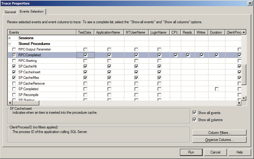
The algebrizer binds the aggregate to the host query and makes its decisions based on query syntax. Consider the following query in the AdventureWorks database:
 SELECT s.CustomerID
 FROM Sales.SalesOrderHeader s
 GROUP BY s.CustomerID
 HAVING EXISTS(SELECT * FROM Sales.Customer c
 WHERE c.TerritoryID > COUNT(s.SalesPersonID))
In this query, although the aggregation is done in the inner query that counts the ContactID, the actual operation of this aggregation is performed in the outer query. For example, in the query plan shown in Figure 13-6, you can see that the aggregation is done on the result from the SalesOrderHeader table although the aggregation is performed in the inner query. The outer query is converted to something like this:
SELECT COUNT(s.SalesPersonID)
 FROM Sales.SalesOrderHeader s
 GROUP BY s.SalesPersonID
Grouping Binding
Consider the following query:
 SELECT s.CustomerID, SalesPersonID, COUNT(s.SalesOrderID)
 FROM Sales.SalesOrderHeader s
 GROUP BY s.CustomerID, s.SalesPersonID
If you do not add the CustomerID and SalesPersonID columns in the GROUP BY list, the query does error out. The grouped queries have different semantics than the nongrouped queries. All nonaggregated columns or expressions in the SELECT list of a query with GROUP BY must have a direct match in the GROUP BY list. The process to verify this via the algebrizer is known as grouping binding.
Optimization
Optimization is probably the most complex and important piece to processing your queries. The logical tree created by the parser and algebrizer is the input to the optimizer. The optimizer needs the logical tree, metadata about objects involved in the query, such as columns, indexes, statistics, and constraints, and hardware information. The optimizer uses this information to create the compiled plan, which is made of physical operators. The logical tree includes logical operators that describe what to do, such as “read table,” “join,” and so on. The physical operators produced by the optimizer specify algorithms that describe how to do, such as “index seek,” “index scan,” “hash join,” and so on. The optimizer tells SQL Server how to exactly carry out the steps to get the results efficiently. Its job is to produce an efficient execution plan for each query in the batch or stored procedure. Figure 13-7 shows this process graphically.

The parser and the algebrizer describe “what to do,” and the optimizer describes “how to do it” (refer to Figure 13-7). SQL Server’s query optimizer is a cost-based optimizer, which means it can create a plan with the least cost. Prior to embarking on a full-blown, cost-based optimization, the query optimizer checks to see if a trivial plan can suffice. A trivial plan is used when the query optimizer knows that there is only one viable plan to satisfy the query. SELECT * FROM <tablename> is one example of this. Complex queries may have millions of possible execution plans. The optimizer does not explore them all though; instead it tries to find a plan that has a cost reasonably close to the theoretical minimum. This is done to come up with a good plan in a reasonable amount of time. Sometimes the query optimization stage ends with a Good Enough Plan Found message or a Time Out. The Good Enough Plan Found message is raised when the query optimizer decides that the current lowest cost plan is so cheap that additional optimization is not worth the cost of doing additional optimization. The Time Out is generated when the optimizer has explored all allowed optimization rules and the optimization stage ends. At that point, the optimizer returns the best complete query plan. The lowest estimated cost doesn’t mean the lowest resource cost. The optimizer chooses the plan to get the results quickly to the users. Suppose the optimizer chooses a parallel plan for your queries that uses multiple CPUs, which typically uses more resources than the serial plan but offers faster results. Of course, the optimizer cannot always come up with the best plan, which is why you have a job — for query tuning.
Optimization Flow
The flowchart in Figure 13-8 explains the steps involved in optimizing a query. These steps are simplified for explanation purposes. (The state-of-the-art optimization engine written by the SQL Server development team isn’t oversimplified.)

The input to the optimizer is a logical tree produced by the algebrizer (refer to Figure 13-8). The query optimizer is a transformation-based engine. These transformations are applied to fragments of the query tree. Three kinds of transformation rules are applied: simplification, exploration, and implementation. The following sections discuss each of these transformations.
Simplification
The simplification process creates an output tree that is more optimized and returns results faster than the input tree. For example, it might push the filter down in the tree, reduce the group by columns, reduce redundant or excessive items in the tree, or perform other transformations. Figure 13-9 shows an example of simplification transformation (filter pushing).

You can see that the logical tree on the left has the filter after the join (refer to Figure 13-9). The optimizer pushes the filter further down in the tree to filter the data out of the Orders table with a predicate on O_OrderPriority. This optimizes the query by performing the filtering early in the execution.
Figure 13-10 is another example of the simplification transformation (aggregate reduction). It differs from Figure 13-9 because it includes reducing the number of Group By columns in the execution plan.
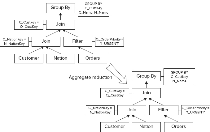
The C_Name column is removed from the Group By clause because it contains the column C_Custkey (refer to Figure 13-7 for the T-SQL statement), which is unique on the Customer table, so there is no need to include the C_Name column in the Group By clause.
Exploration
As mentioned previously, SQL Server uses a cost-based optimizer implementation. Therefore, during the exploration process, the optimizer looks at alternative options to come up with the cheapest plan (see Figure 13-11). It makes a global choice using the estimated cost.

The optimizer explores the options related to which table should be used for inner versus outer joins. This is not a simple determination because it depends on many things, such as the size of the table, the available indexes, statistics, and operators higher in the tree. It is not a clear choice like the examples you saw in the simplification transformation.
Implementation
The third transformation is implementation. Figure 13-12 shows an example.

As explained earlier, the implantation transforms the “what to do” part into the “how to do” part. In this example, the JOIN logical operation transforms into a HASH JOIN physical operation. The query cost is derived from physical operators based on model-of-execution algorithms (I/O and CPU) and estimations of data distribution, data properties, and size. Needless to say, the cost also depends on hardware such as the number of CPUs and the amount of memory available at the time of optimization.
Refer back to Figure 13-8. If the optimizer compared the cost of every valid plan and chose the least costly one, the optimization process could take a long time, and the number of valid plans could be huge. Therefore, the optimization process is divided into three search phases. As discussed earlier, a set of transformation rules is associated with each phase. After each phase, SQL Server 2012 evaluates the cost of the cheapest query plan to that point. If the plan is cheap enough, then the optimizer stops there and chooses that query plan. If the plan is not cheap enough, the optimizer runs through the next phase, which has an additional set of rules that are more complex.
The first phase of the cost-based optimization, Phase 0, contains a limited set of rules. These rules are applied to queries with at least four tables. Because JOIN reordering alone generates many valid plans, the optimizer uses a limited number of join orders in Phase 0 and considers only hash and loop joins in this phase. In other words, if this phase finds a plan with an estimated cost below 0.2 (internal cost unit), the optimization ends there.
The second phase, Phase 1, uses more transformation rules and different join orders. The best plan that costs less than 1.0 would cause optimization to stop in this phase. Until Phase 1, the plans are nonparallel (serial query plans).
Consider this: What if you have more than one CPU in your system? In that case, if the cost of the plan produced in Phase 1 is more than the cost threshold for parallelism (see sp_configure for this parameter; the default value is 5), then Phase 1 is repeated to find the best parallel plan. Then the cost of the serial plan produced earlier is compared with the new parallel plan, and the next phase, Phase 2 (the full optimization phase), is executed for the cheaper of the two plans.
PHYSICAL QUERY PROCESSING PART TWO: EXECUTION
After compilation, the execution engine takes over; it generates the execution plan, it copies the plan into its executable form and executes the steps in the query plan to produce the wanted result. If the same query or stored procedure is executed again, the compilation phase is skipped, and the execution engine uses the same cached plan to start the execution. Once that is complete, the data needs to be accessed and there are a myriad of ways to perform that index access. There is always room for tuning, but you must have enough data to start with. Therefore, you need to take a baseline of the system’s performance and compare against that baseline so that you know where to start. Chapter 12, “Monitoring Your SQL Server,” has details on getting the baseline. Just because a process is slow doesn’t mean that you have to start tuning SQL statements. First you need to do many basic things, such as configure the SQL Server 2012 database, and make sure tempdb and the log files are on their own drives. It is important to get the server configuration correct. See Chapter 10, “Configuring the Server for Optimal Performance,” and Chapter 11, “Optimizing SQL Server 2012,” for details about configuring your server and database for optimal performance. There is also a white paper on tempdb that you should read. This document is for SQL Server 2005, but it’s useful for SQL Server 2012 as well and can be found at: www.microsoft.com/technet/prodtechnol/sql/2005/workingwithtempdb.mspx.
Don’t overlook the obvious. For example, suppose you notice that performance is suddenly quite bad on your server. If you have done a baseline and that doesn’t show much change in performance, then it is unlikely that the sudden performance change was caused by an application in most cases, unless a new patch for your application caused some performance changes. In that case, look at your server configuration to see if that changed recently. Sometimes you merely run out of disk space, especially on drives where your page files reside, and that can bring the server to its knees.
Database I/O Information
Normally, an enterprise application has one or two databases residing on the server, in which case you would know that you need to look into queries against those databases. Each query may require a high level of I/O and, ideally, would like to take the maximum level of I/O available to entire server. However, if you have many databases on the server and you are not sure which database is causing a lot of I/O and may be responsible for a performance issue, you must look at the I/O activities against the database to find out which causes the most I/O and stalls on the I/O and how that can affect the execution time of your specific query. The DMF called sys.dm_io_virtual_file_stats comes in handy for this purpose.
Listing 13-4 provides this information.
LISTING 13-4: DatabseIO.sql
-- Database IO analysis.
WITH IOFORDATABASE AS
(
SELECT
 DB_NAME(VFS.database_id) AS DatabaseName
,CASE WHEN smf.type = 1 THEN 'LOG_FILE' ELSE 'DATA_FILE' END AS DatabaseFile_Type
,SUM(VFS.num_of_bytes_written) AS IO_Write
,SUM(VFS.num_of_bytes_read) AS IO_Read
,SUM(VFS.num_of_bytes_read + VFS.num_of_bytes_written) AS Total_IO
,SUM(VFS.io_stall) AS IO_STALL
FROM sys.dm_io_virtual_file_stats(NULL, NULL) AS VFS
JOIN sys.master_files AS smf
  ON VFS.database_id = smf.database_id
 AND VFS.file_id = smf.file_id
GROUP BY
 DB_NAME(VFS.database_id)
,smf.type
)
SELECT
 ROW_NUMBER() OVER(ORDER BY io_stall DESC) AS RowNumber
,DatabaseName
,DatabaseFile_Type
,CAST(1.0 * IO_Read/ (1024 * 1024) AS DECIMAL(12, 2)) AS IO_Read_MB
,CAST(1.0 * IO_Write/ (1024 * 1024) AS DECIMAL(12, 2)) AS IO_Write_MB
,CAST(1. * Total_IO / (1024 * 1024) AS DECIMAL(12, 2)) AS IO_TOTAL_MB
,CAST(IO_STALL / 1000. AS DECIMAL(12, 2)) AS IO_STALL_Seconds
,CAST(100. * IO_STALL / SUM(IO_STALL) OVER() AS DECIMAL(10, 2)) AS IO_STALL_Pct
FROM IOFORDATABASE
ORDER BY IO_STALL_Seconds DESC
Figure 13-13 shows sample output from this script.

The counters can be explained as such:
- DatabaseName: Name of the database
- DatabaseFile_Type: Data file or Log file for the associated database name
- IO_Read_MB: Number of bytes read from the database file
- IO_Write_MB: Number of bytes written to the database file
- IO_TOTAL_MB: Total number of bytes transferred to/from the database file
- IO_STALL_Seconds: Time, in seconds, that users waited for I/O to be completed on the file
- IO_STALL_Pct: IO stall percentage relative to the entire query
The counters show the value from the time the instance of SQL Server starts, but it gives you a good idea of which database is hammered. This query gives you a good starting point to further investigate the process level (stored procedures, ad-hoc T-SQL statements, and so on) for the database in question.
Next, look at how to gather the query plan and analyze it. You also learn about the different tools you need in this process.
Working with the Query Plan
Looking at the query plan is the first step to take in the process of query tuning. The SQL Server query plan comes in different flavors: textual, graphical, and, with SQL Server 2012, XML format. Showplan describes any of these query plan flavors. Different types of Showplans have different information. SQL Server 2012 can produce a plan with operators only, with cost information, and with XML format, which can provide some additional runtime details. Table 13-2 summarizes the various Showplan formats.
TABLE 13-2: Showplan Formats

Estimated Execution Plan
This section describes how to get the estimated execution plan. In a later section you learn how to get the actual execution plan. There are five ways you can get the estimated execution plan:
- SET SHOWPLAN_TEXT
- SET SHOWPLAN_ALL
- SET SHOWPLAN_XML
- Graphical estimated execution plan using SQL Server Management Studio (SSMS)
- SQL Trace
The SQL Trace option is covered in a separate section at the end of the chapter; the other options are described in the following sections.
SET SHOWPLAN_TEXT and SET SHOWPLAN_ALL
Start with a simple query to demonstrate how to read the query plan. The code for the query is shown in Listing 13-5:
LISTING 13-5: SimpleQueryPlan.sql
USE AdventureWorks
GO
SET SHOWPLAN_TEXT ON
GO
SELECT sh.CustomerID, st.Name, SUM(sh.SubTotal) AS SubTotal
FROM Sales.SalesOrderHeader sh
JOIN Sales.Customer c
  ON c.CustomerID = sh.CustomerID
JOIN Sales.SalesTerritory st
  ON st.TerritoryID = c.TerritoryID
GROUP BY sh.CustomerID, st.Name
HAVING SUM(sh.SubTotal) > 2000.00
GO
SET SHOWPLAN_TEXT OFF
GO
When you SET the SHOWPLAN_TEXT ON, the query does not execute; it just produces the estimated plan. The textual plan is shown next.
The output tells you that there are seven operators: Filter, Hash Match (Inner Join), Hash Match (Aggregate), Clustered Index Scan, Merge Join, Clustered Index Scan, and Index Scan, which are shown in bold in the query plan here.
SELECT sh.CustomerID, st.Name, SUM(sh.SubTotal) AS SubTotal
FROM Sales.SalesOrderHeader sh
   JOIN Sales.Customer c
     ON c.CustomerID = sh.CustomerID
   JOIN Sales.SalesTerritory st
     ON st.TerritoryID = c.TerritoryID
   GROUP BY sh.CustomerID, st.Name   HAVING SUM(sh.SubTotal) > 2000.00

StmtText
  |--Filter(WHERE:([Expr1006]>(2000.00)))
       |--Hash Match(Inner Join, HASH:([st].[TerritoryID])=([c].[TerritoryID]),
RESIDUAL:([AdventureWorks].[Sales].[SalesTerritory].[TerritoryID]
as [st].[TerritoryID]=[AdventureWorks].[Sales].[Customer].[TerritoryID]
as [c].[TerritoryID]))
            |--Clustered Index
Scan(OBJECT:([AdventureWorks].[Sales].[SalesTerritory].
[PK_SalesTerritory_TerritoryID] AS [st]))
            |--Hash Match(Inner Join, HASH:([sh].[CustomerID])=([c].[CustomerID]))
                 |--Hash Match(Aggregate, HASH:([sh].[CustomerID]) DEFINE:
([Expr1006]=SUM([AdventureWorks].[Sales].[SalesOrderHeader].[SubTotal]
as [sh].[SubTotal])))
                 |    |--Clustered Index Scan(OBJECT:
([AdventureWorks].[Sales].[SalesOrderHeader].
[PK_SalesOrderHeader_SalesOrderID] AS [sh]))
                 |--Index Scan(OBJECT:
([AdventureWorks].[Sales].[Customer].[IX_Customer_TerritoryID]
AS [c]))
It may be easier to view the plan output in SSMS since the formatting here doesn’t look that good. You can run this query in the AdventureWorks database. In this plan all you have are the operators’ names and their basic arguments. For more details on the query plan, other options are available, which you explore soon.
To analyze the plan you read branches in inner levels before outer ones (bottom to top), and branches that appear in the same level from top to bottom. You can tell which branches are inner and which are outer based on the position of the pipe (|) character. When the plan executes, the general flow of the rows is from the top down and from right to left. An operator with more indentation produces rows consumed by an operator with less indentation and produces rows for the next operator above, and so forth. For the JOIN operators, two input operators exist at the same level to the right of the JOIN operator, denoting the two row sets. The higher of the two (in this case, Clustered Index Scan on the object Sales.SalesTerritory) is the outer table (so Sales.SalesTerritory is the outer table) and the lower (Index Scan on the object Sales.Customer) is the inner table. The operation on the outer table is initiated first, and the one on the inner table is repeatedly executed for each row of the outer table that arrives to the join operator. The join algorithms are explained in detail later.
Now you can analyze the plan for the query. As shown in the plan, the hash match (inner join) operation has two levels: hash match (aggregate) and merge join. Now look at the merge join. The merge join has two levels: The first is the clustered index scan on Sales.Territory, and the index scanned on this object is PK_SalesTerritory_TerritoryID. You explore index access methods in more detail a little later in the chapter. That is the outer table for the merge join. The inner table Sales.Customer is scanned only once because of the merge join, and that physical operation is done using an index scan on index IX_Customer_TerritoryID on the sales.Customer table. The merge join is on the TerritoryID, as per the plan Merge Join(Inner Join, MERGE:([st].[TerritoryID]) = ([c].[TerritoryID]). Because the RESIDUAL predicate is present in the merge join, all rows that satisfy the merge predicate evaluate the residual predicate, and only those rows that satisfy it are returned.
Now the result of this merge join becomes the inner table for hash match (inner join): Hash Match (Inner Join, HASH:([sh].[CustomerID]) = ([c].[CustomerID])). The outer table is the result of Hash Match (Aggregate). You can see that the CustomerID is the hash key (HASH:([sh].[CustomerID]) in the hash aggregate operation. Therefore, the aggregation is performed and, as per the query, the SUM operation is done on the column SubTotal from the Sales.SalesOrderHeader table (defined by the DEFINE:([Expr1006]). Now the Hash Match (Inner join) operation is performed on CustomerID (the result of the merge join) repeatedly for each row from the outer table (the result of hash match [aggregate]). Finally, the filter is applied on column SubTotal using the filter physical operator with the predicate (WHERE:([Expr1006]>(2000.00)))to get only rows with SubTotal > 2000.00.
The merge join itself is fast, but it can be an expensive choice if sort operations are required. However, if the data volume is large and the wanted data can be obtained presorted from existing B-tree indexes, Merge Join is often the fastest available join algorithm. In addition, Merge Join performance can vary a lot based on one-to-many or many-to-many joins.
In the query file, you set the SET SHOWPLAN_TEXT OFF following the query. This is because SET SHOWPLAN_TEXT ON is not only causing the query plan to show up, but it is also turning off the query execution for the connection. The query execution is turned off for this connection until you execute SET SHOWPLAN_TEXT OFF on the same connection. The SET SHOWPLAN_ALL command is similar to SET SHOWPLAN_TEXT. The only difference is the additional information about the query plan produced by SET SHOWPLAN_ALL. It adds the estimated number of rows produced by each operator in the query plan, the estimated CPU time, the estimated I/O time, and the total cost estimate that was used internally when comparing this plan to other possible plans.
SET SHOWPLAN_XML
The SET SHOWPLAN_XML feature was added in SQL Server 2005 to retrieve the Showplan in XML form. The output of the SHOWPLAN_XML is generated by a compilation of a batch, so it produces a single XML document for the whole batch. See Listing 13-6 to see how you can get the estimated plan in XML.
LISTING 13-6: ShowPlan_XML.sql
USE AdventureWorks
GO
SET SHOWPLAN_XML ON
GO
SELECT sh.CustomerID, st.Name, SUM(sh.SubTotal) AS SubTotal
FROM Sales.SalesOrderHeader sh
JOIN Sales.Customer c
  ON c.CustomerID = sh.CustomerID
JOIN Sales.SalesTerritory st
  ON st.TerritoryID = c.TerritoryID
GROUP BY sh.CustomerID, st.Name
HAVING SUM(sh.SubTotal) > 2000.00
GO
SET SHOWPLAN_XML OFF
GO
When you run this query in Management Studio, you can see a link in the result tab. Click the link to open the XML document inside Management Studio and save that document with the extension .sqlplan. When you open that file using Management Studio, you get a graphical query plan. Figure 13-14 shows the graphical plan from the XML document generated by this query.

XML is the richest format of the Showplan. It contains some unique information not available in other Showplan formats. The XML Showplan contains the size of the plan in cache (the CachedPlanSize attributes) and parameter values for which the plan has been optimized (the Parameter sniffing element). When a stored procedure compiles for the first time, the values of the parameters supplied with the execution call optimize the statements within that stored procedure. This process is known as parameter sniffing. Also available is some runtime information, which is unique to the XML plan and described further in the section, “Actual Execution Plan” later in this chapter.
You can write code to parse and analyze the XML Showplan. This is probably the greatest advantage it offers because this task is hard to achieve with other forms of the Showplan.
Refer to the white paper at http://msdn.microsoft.com/en-us/library/ms345130.aspx for information on how you can extract the estimated execution cost of a query from its XML Showplan using CLR functions. This document is for SQL Server 2005 but still applies. You can use this technique to ensure that users can submit only those queries costing less than a predetermined threshold to a server running SQL Server, thereby ensuring it is not overloaded with costly, long-running queries.
Graphical Estimated Showplan
You can view a graphical estimated plan in Management Studio. To access the plan, either use the shortcut key Ctrl+L or select Query ![]() Display Estimated Execution plan. You can also select the button indicated in Figure 13-15.
Display Estimated Execution plan. You can also select the button indicated in Figure 13-15.

If you use any of these options to display the graphical estimated query plan, it displays the plan as soon as compilation is completed because compilation complexity can vary according to the number and size of the tables. Right-clicking the graphical plan area in the Execution Plan tab reveals different zoom options and properties for the graphical plan.
Actual Execution Plan
This section describes the options you can use to get the actual execution plan (SET STATISTICS XML ON|OFF and SET STATISTICS PROFILE ON|OFF) using the graphical actual execution plan option in Management Studio. You can get the actual execution plan using SQL Trace as well; see the section, “Gathering Query Plans for Analysis with SQL Trace” later in this chapter.
SET STATISTICS XML ON|OFF
Two kinds of runtime information are in the XML Showplan: per SQL statement and per thread. If a statement has a parameter, the plan contains the parameterRuntimeValue attribute, which shows the value of each parameter when the statement was executed. The degreeOfParallelism attribute shows the actual degree of parallelism. The degree of parallelism shows the number of concurrent threads working on the single query. The compile time value for degree of parallelism is always half the number of CPUs available to SQL Server unless two CPUs are in the system. In that case, the value will be 2 as well.
The XML plan may also contain warnings. These are events generated during compilation or execution time. For example, missing statistics are a compiler-generated event. One important feature in SQL Server 2012 (originally added in SQL Server 2005) is the USE PLAN hint. This feature requires the plan hint in XML format, so you can use the XML Showplan. Using the USE PLAN hint, you can force the query to be executed using a certain plan. For example, suppose you find that a query runs slowly in the production environment but faster in the preproduction environment. You also find that the plan generated in the production environment is not optimal for some reason. In that case, you can use the better plan generated in the preproduction environment and force that plan in the production environment using the USE PLAN hint. For more details on how to implement it, refer to the Books Online (BOL) topic, “Using the USE PLAN Query Hint.”
There are new warnings that have been included in SQL Server 2012 execution plan. These two messages specifically warn against implicit (or, sometimes, explicit) type conversions that cause the available index not to be used. The first warning message is:
 Type conversion in expression ColumnExpression may affect
"CardinalityEstimate" in query plan choice
This means that there is a type conversion on a certain column that will affect the CardinalityEstimate. The other warning message is:
Type conversion in expression ColumnExpression may affect
"SeekPlan" in query plan choice.
This means that the type conversion that is happening on a certain column will cause the index not to be used.
SET STATISTICS PROFILE ON|OFF
The SET STATISTICS PROFILE ON|OFF option is better than the previous option, which you should use it for query analysis and tuning. Run the following query using the code shown in Listing 13-7. If you don’t want to mess with your AdventureWorks database, you can back up and restore the AdventureWorks database with a different name. If you do that, be sure to change the USE DatabaseName line in the script.
LISTING 13-7: Statistics_Profile.sql
USE AdventureWorks
GO
SET STATISTICS PROFILE ON
GO
SELECT p.Name AS ProdName, c.TerritoryID, SUM(od.OrderQty)
FROM Sales.SalesOrderDetail od
JOIN Production.Product p
  ON p.ProductID = od.ProductID
JOIN Sales.SalesOrderHeader oh
  ON oh.SalesOrderID = od.SalesOrderID
JOIN Sales.Customer c
  ON c.CustomerID = oh.CustomerID
WHERE OrderDate >= '2006-06-09'
  AND OrderDate <= '2006-06-11'
GROUP BY p.Name, c.TerritoryID
GO
SET STATISTICS PROFILE OFF
After you run the query, you get output similar to what is shown in Figure 13-16.

The four most important columns in the output of SET STATISTICS PROFILE are Rows, EstimateRows, Executes, and, of course, the StmtText. The Rows column contains the number of rows actually returned by each operator.
Graphical Actual Execution Plan
You can use Management Studio to view the graphical actual execution plan. Again, either use the shortcut Ctrl+M, select Query ![]() Include Actual Execution plan, or select the button indicated in Figure 13-17.
Include Actual Execution plan, or select the button indicated in Figure 13-17.
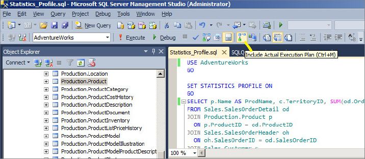
If you use any of these options to display the graphical actual query plan, nothing happens. After query execution, the actual plan displays in a separate tab.
Index Access Methods
There are a number of index access methods that SQL Server uses to retrieve data needed to build execution plans. In this section you get to explore the ways that these methods are different from each other and how the index access methods may affect the performance of the query. You can use this knowledge when you tune the query and decide whether it uses the correct index access method and take the appropriate action.
In addition, you should make a copy (Backup and Restore, or take a snapshot) of the AdventureWorks database on your machine so that if you drop or create indexes on it, the original AdventureWorks database remains intact. When you restore the database, call it AW_2 for these examples.
Table Scan
A table scan involves a sequential scan of all data pages belonging to the table. Run the following script in the AW_2 database:
SELECT * INTO dbo.New_SalesOrderHeader
FROM Sales.SalesOrderHeader
After you run this script to make a copy of the SalesOrderHeader table, run the following script:
SELECT SalesOrderID, OrderDate, CustomerID
FROM dbo.New_SalesOrderHeader
Because this is a heap, this statement causes a table scan. If you want, you can always get the actual textual plan using SET STATISTICS PROFILE ON. Figure 13-18 displays the graphical plan.
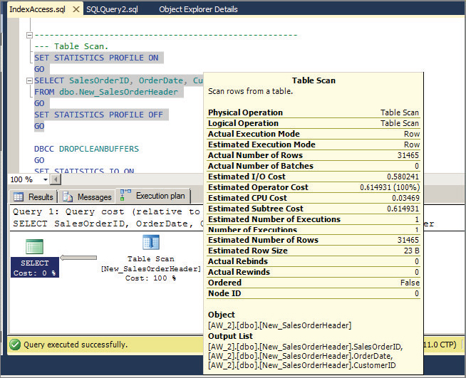
In a table scan, SQL Server uses Index Allocation Map (IAM) pages to direct the disk arm to scan the extents belonging to the table according to their physical order on disk. As you might guess, the number of physical reads would be the same as the number of pages for this table.
Now look at the STATISTICS IO output for the example query in Listing 13-8. This is a session-level setting. STATISTICS IO provides you with I/O-related statistics for the query statement that caused a table scan which was run.
SET STATISTICS IO is set at runtime and not at parse time. This is an important tool in your query-tuning arsenal because disk I/O is normally a bottleneck on your system, so you must to identify how many I/O’s your query generates and whether they are necessary.
LISTING 13-8: IndexAccess1.sql
DBCC DROPCLEANBUFFERS
GO
SET STATISTICS IO ON
GO
SELECT SalesOrderID, OrderDate, CustomerID
FROM dbo.New_SalesOrderHeader
GO
SET STATISTICS IO OFF
The statistics I/O information is as follows:
Table 'New_SalesOrderHeader'. Scan count 1, logical reads 794,
physical reads 0, read-ahead reads 276, lob logical reads 0,
lob physical reads 0, lob read-ahead reads 0.
The scan count tells you how many times the table was accessed for this query. If you have multiple tables in your query, you see statistics showing I/O information for each table. In this case, the New_SalesOrderHeader table was accessed once.
The logical reads counter indicates how many pages were read from the data cache. In this case, 794 reads were done from cache. The logical reads number may be a little different on your machine. As mentioned earlier, because of the whole table scan, the number of logical reads equals the number of pages allocated to this table.
You can also run the following query to verify the number of pages allocated to the table.
select in_row_reserved_page_count
from sys.dm_db_partition_stats
 WHERE OBJECT_ID = OBJECT_ID('New_SalesOrderHeader')
The physical reads counter indicates the number of pages read from the disk. It shows 0 for the preceding code. This doesn’t mean that there were no physical reads from disk though.
The read-ahead reads counter indicates the number of pages from the physical disk that are placed into the internal data cache when SQL Server guesses that you will need them later in the query. In this case, this counter shows 276, which is the total number of physical reads that occurred. Both the physical reads and read-ahead reads counters indicate the amount of physical disk activity. These numbers may, too, be different on your machine.
The lob logical reads, lob physical reads, and lob read-ahead reads are the same as the other reads, but these counters indicate reads for the large objects — for example, if you read a column with the data types varchar(max), nvarchar(max), xml, or varbinary(max). When T-SQL statements retrieve lob columns, some lob retrieval operations might require traversing the lob tree multiple times. This may cause SET STATISTICS IO to report higher than expected logical reads.
Clustered Index Scan (Unordered)
Try creating a clustered index on the New_SalesOrderHeader table. A clustered index is structured as a balanced tree. (Most indexes in SQL Server are traditionally structured as balanced trees. New indexes found in SQL Server 2012, such as ColumnStore, full-text, and spatial indexes are not.) A balanced tree is one in which “no leaf is much farther away from the root than any other leaf” (adopted from www.nist.gov/dads/HTML/balancedtree.html). Different balancing schemes allow different definitions of “much farther” and different amounts of work to keep them balanced. A clustered index maintains the entire table’s data at its leaf level.
A clustered index is not a copy of the table’s data; it is the data.
Now run the script in Listing 13-9 and query to see the effect of adding a clustered index.
LISTING 13-9: IndexAccess2.sql
CREATE CLUSTERED INDEX IXCU_SalesOrderID ON New_SalesOrderHeader(SalesOrderID)
GO
DBCC DROPCLEANBUFFERS
GO
SET STATISTICS IO ON
GO
SELECT SalesOrderID, RevisionNumber, OrderDate, DueDate
FROM New_SalesOrderHeader
GO
SET STATISTICS IO OFF
The results of Statistics IO are shown here, and the query plan is shown in Figure 13-19:

Table 'New_SalesOrderHeader'. Scan count 1, logical reads 794,
physical reads 0, read-ahead reads 276, lob logical reads 0,
lob physical reads 0, lob read-ahead reads 0.
As shown in the Statistics IO output, the number of pages read was 794 (logical reads), which is the same as the table scan (a little more actually because the leaf level in a clustered index also contains unique row information plus a link to the previous and next page in a doubly linked list, so more space is required to hold that information). Even though the execution plan shows a clustered index scan, the activities are the same as the table scan, so unless you have a predicate on a clustered index key, the whole clustered index will be scanned to get the data, which is the same as a table scan. You can also see in Figure 13-19, in the information box of the clustered index scan operators, that the scan was not ordered (Ordered = False), which means that the access method did not rely on the linked list between the data pages and the leaf-level that maintains the logical order of the index.
Clustered Index Scan (Ordered)
An ordered clustered index scan is also a full scan of the clustered index, but the data is returned in order by the clustering key. This time, run the query found in Listing 13-10. This query can access the same table but is ordered by the SalesOrderID column:
LISTING 13-10: IndexAccess3.sql
DBCC DROPCLEANBUFFERS
GO
SET STATISTICS IO ON
GO
SELECT SalesOrderID,RevisionNumber, OrderDate, DueDate
FROM New_SalesOrderHeader
ORDER BY SalesOrderID
GO
SET STATISTICS IO OFF
The statistics I/O information is as follows:
Table 'New_SalesOrderHeader'. Scan count 1, logical reads 794,
physical reads 0, read-ahead reads 276, lob logical reads 0,
lob physical reads 0, lob read-ahead reads 0.
The query plan is shown in Figure 13-20.

As you can see, the query plan is the same in Figure 13-20 as the one in Figure 13-19, but here you have Ordered = True. The statistics IO information is also the same as the unordered clustered index scan. Unlike the unordered clustered index scan, the performance of the ordered clustered index scan depends on the fragmentation level of the index. Fragmentation is out-of-order pages, which means that although Page 1 appears after Page 2 according to the linked list, physically Page 2 comes before Page 1 on the disk, or there is a gap in sequential pages. It is more expensive to swing back but gaps going forward can affect the size of the reads. The percentage of fragmentation is greater if more pages in the leaf level of the index are out of order with respect to the total number of pages. Moving the disk arm sequentially is always faster than random arm movement, so if the fragmentation is higher than for ordered data, there will be more random arm movement, resulting in slower performance.
If you do not need the data sorted, do not include the ORDER BY clause.
Even though you have a covering non-clustered index, the optimizer in Figure 13-19 did not choose it this time because you asked that the data be sorted on the SalesOrderID column (which is obviously not sorted on the leaf level of the non-clustered index).
Covering Non-Clustered Index Scan (Unordered)
A covering index means that a non-clustered index contains all the columns specified in a query. Look at this using the query used in Listing 13-11:
LISTING 13-11: IndexAccess4.sql
CREATE NONCLUSTERED INDEX IXNC_SalesOrderID ON New_SalesOrderHeader(OrderDate)
INCLUDE(RevisionNumber, DueDate)
GO
DBCC DROPCLEANBUFFERS
GO
SET STATISTICS IO ON
GO
SELECT SalesOrderID, RevisionNumber, OrderDate, DueDate
FROM New_SalesOrderHeader
GO
SET STATISTICS IO OFF
This script creates a non-clustered index on the OrderDate column. Notice the INCLUDE clause with the column names RevisionName and DueDate. The INCLUDE feature, introduced in SQL Server 2005, enables you to specify the non-key columns to be added to the leaf level of the non-clustered index. The RevisionName and DueDate columns are included because your query needs these columns. The non-clustered index is chosen for this operation so that the data can be served directly from the leaf level of the non-clustered index (because the non-clustered index has the data for these included columns). See the CREATE INDEX topic in BOL for details on the INCLUDE clause. The statistics I/O information for the query is shown here:
Table 'New_SalesOrderHeader'. Scan count 1, logical reads 108,
physical reads 0, read-ahead reads 0, lob logical reads 0,
lob physical reads 0, lob read-ahead reads 0.
The query plan is shown in Figure 13-21.

As you can see from the statistics I/O result, only 108 logical reads were done to fulfill this query. The results returned by the clustered index query and the covering non-clustered index query are identical (number of columns and number of rows), but there were 794 logical reads in the clustered index and only 108 logical reads in the non-clustered scan because the non-clustered index has covered the query and served the data from its leaf level.
The clustered index leaf level contains the full data rows (all columns), whereas the non-clustered index has only one key column and two included columns. That means the row size is smaller for a non-clustered index, and the smaller row size can hold more data and requires less I/O.
Covering Non-Clustered Index Scan (Ordered)
If you run the query found in Listing 13-11 with OrderDate in the ORDER BY clause, the optimizer chooses the covering non-clustered index. The query plan would be exactly the same as shown in Figure 13-21, except that you see Ordered = True in the information box. The statistics IO information is also the same as for the non-ordered covering non-clustered index scan. Of course, an ordered index scan is not only used when you explicitly request the data sorted; the optimizer can also choose to sort the data if the plan uses an operator that can benefit from sorted data.
Non-Clustered Index Seek with Ordered Partial Scan and Lookups
To demonstrate the non-clustered index seek with ordered partial scan and lookups access method, you first need to drop the clustered index on the New_SalesOrderHeader table. Run the script in Listing 13-12:
LISTING 13-12: IndexAccess5.sql
DROP INDEX New_SalesOrderHeader.IXCU_SalesOrderID
GO
DBCC DROPCLEANBUFFERS
GO
SET STATISTICS IO ON
GO
SELECT SalesOrderID,RevisionNumber, OrderDate, DueDate
FROM New_SalesOrderHeader
WHERE OrderDate BETWEEN '2007-10-08 00:00:00.000' AND '2007-10-10 00:00:00.000'
GO
SET STATISTICS IO OFF
The statistics IO looks like this:
(186 row(s) affected)
Table 'New_SalesOrderHeader'. Scan count 1, logical reads 188,
physical reads 0, read-ahead reads 0, lob logical reads 0,
lob physical reads 0, lob read-ahead reads 0.
The query execution plan is shown in Figure 13-22.

Remember that you don’t have a clustered index on this table. This is called a heap. In the query, you have requested the SalesOrderID, RevisionNumber, OrderDate, DueDate, and SalesOrderNumber columns, and added a predicate on the OrderDate column. Because of the predicate on the key column in the IXNC_SalesOrderID index, the optimizer chooses this index and looks for all the rows that have the OrderDate specified in the WHERE clause. This index also has all the columns at its leaf level except for SalesOrderID. To find the SalesOrderID column value, SQL Server performs RID lookups of the corresponding data row for each key. As each key is found, SQL Server can apply the lookup. In addition, because this is a heap table, each lookup translates to a single page read. Because there are 186 rows qualified by the WHERE clause, there will be 186 reads for data row lookup. If you look at the statistics IO information, there are 188 logical reads, which means that out of those 188 logical reads, 186 are the result of the RID lookup. You can probably guess that most of the cost in this query is in the RID lookup, which is also evident in the query plan, which shows that the cost of the RID lookup operation is 99 percent. Lookups are always random I/Os (as opposed to sequential), which are more costly. When seeking many times, however, SQL Server often sorts to make I/Os more sequential.
This query plan demonstrated an RID lookup on a heap. Run the script in Listing 13-13 to create a clustered index and run the same query again:
LISTING 13-13: IndexAccess6.sql
CREATE CLUSTERED INDEX IXCU_SalesOrderID ON New_SalesOrderHeader(SalesOrderID)
GO
DBCC DROPCLEANBUFFERS
GO
SET STATISTICS IO ON
GO
SELECT SalesOrderID,RevisionNumber, OrderDate, DueDate, SalesOrderNumber
FROM New_SalesOrderHeader
WHERE OrderDate BETWEEN '2007-10-08 00:00:00.000' AND '2007-10-10 00:00:00.000'
GO
SET STATISTICS IO OFF
The following code shows the statistics IO output for this query:
(186 row(s) affected)
Table 'New_SalesOrderHeader'. Scan count 1, logical reads 581,
physical reads 0, read-ahead reads 5, lob logical reads 0,
lob physical reads 0, lob read-ahead reads 0.
Figure 13-23 shows the query plan for this query.
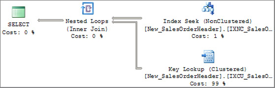
The query plans in Figure 13-22 and Figure 13-23 are almost identical except that in Figure 13-23 a clustered index is sought for each row found in the outer reference (the non-clustered index). Again, you can see in Figure 13-23 that the clustered index seek incurs most of the cost (99 percent) for this query, but note the statistics IO information for the two queries. The logical reads in the clustered index seek query plan are a lot higher than those in the RID lookup plan. This doesn’t mean that a clustered index on the table is bad, though. This index access method is efficient only when the predicate is highly selective, or a point query. Selectivity is defined as the percentage of the number of rows returned by the query out of the total number of rows in the table. A point query is one that has an equals (=) operator in the predicate. Because the cost of the lookup operation is greater, the optimizer decided to just do the clustered index scan. For example, if you change the WHERE clause in the query to WHERE OrderDate BETWEEN '2007-10-08 00:00:00.000' AND '2007-12-10 00:00:00.000', then the optimizer would just do the clustered index scan to return the result for that query. Remember that the non-leaf levels of the clustered index typically reside in cache because of all the lookup operations going through it, so you shouldn’t concern yourself too much about the higher cost of the query in the clustered index seek scenario shown in Figure 13-23.
Clustered Index Seek with Ordered Partial Scan
The optimizer normally uses the clustered index seek with an ordered partial scan technique for range queries, in which you filter based on the first key column of the clustered index. To observe this technique, run the query in Listing 13-14:
LISTING 13-14: IndexAccess7.sql
DBCC DROPCLEANBUFFERS
GO
SET STATISTICS IO ON
GO
SELECT SalesOrderID, RevisionNumber, OrderDate, DueDate, SalesOrderNumber
FROM New_SalesOrderHeader
WHERE SalesOrderID BETWEEN 43696 AND 45734
GO
SET STATISTICS IO OFF
The statistics IO output is as follows:
(2039 row(s) affected)
Table 'New_SalesOrderHeader'. Scan count 1, logical reads 56,
physical reads 0, read-ahead reads 0, lob logical reads 0,
lob physical reads 0, lob read-ahead reads 0.
The query plan is shown in Figure 13-24.
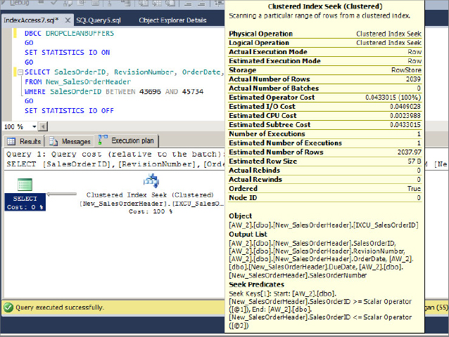
This index access method first performs a seek operation on the first key (43696 in this case) and then performs an ordered partial scan at the leaf level, starting from the first key in the range and continuing until the last key (45734). Because the leaf level of the clustered index is actually the data rows, no lookup is required in this access method.
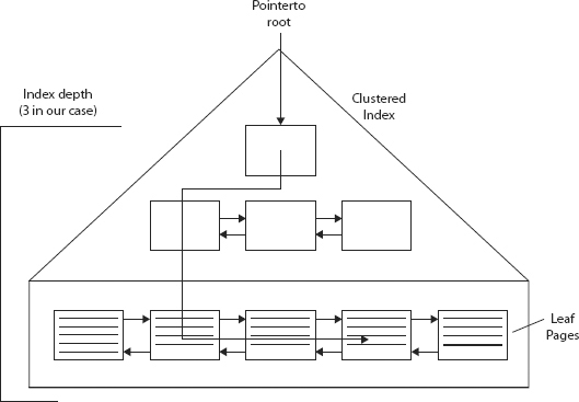
Look at Figure 13-25 to understand the I/O cost for this index access method. To read at least a single leaf page, the number of seek operations required is equal to the number of levels in the index.
How do you find the level in the index? Run the INDEXPROPERTY function with the IndexDepth property:
 SELECT INDEXPROPERTY (OBJECT_ID('New_SalesOrderHeader'), 'IXCU_SalesOrderID',
 'IndexDepth')
In this case, the index depth is 3, and of course the last level is the leaf level where the data resides. As shown in Figure 13-25, the cost of the seek operation (three random reads in this case because that is the depth of the index) and the cost of the ordered partial scan within the leaf level to get the data (in this case 53, according to the read-ahead reads) add up to 56 logical reads, as indicated in the statistics IO information. As you can see, an ordered partial scan typically incurs the bulk of the query’s cost because it involves most of the I/O to scan the range (53 in this case). As mentioned earlier, index fragmentation plays an important role in ordered partial scan operations, so when there is high fragmentation in the index, the disk arm needs to move a lot, which results in degraded performance.
The query plan shown in Figure 13-24 is called a trivial plan, which means that there is no better plan than this and the plan does not depend on the selectivity of the query. As long as you have a predicate on the SalesOrderID columns, no matter how many rows are sought, the plan is always the same unless you have a better index that the query optimizer can choose from.
Fragmentation
Throughout this chapter, there have been a number of places in which fragmentation was mentioned. Most specifically, in the difference between ordered and unordered index scans, you looked at how fragmentation can affect the performance of the query due to the order of pages and extents in a table. The following section elaborates on this. The two types of fragmentation are logical scan fragmentation and average page density. Logical scan fragmentation is the percentage of out-of-order pages in the index in regard to their physical order, rather than their logical order, in the linked list. This fragmentation has a substantial impact on ordered scan operations like the one shown in Figure 13-24. This type of fragmentation has no impact on operations that do not rely on an ordered scan, such as seek operations, unordered scans, or lookup operations.
The average page density is the percentage of pages that are full. A low percentage (fewer pages full) has a negative impact on the queries that read the data because these queries end up reading more pages than they could, were the pages better populated. The upside of having free space in pages is that insert operations in these pages do not cause page splits, which are expensive and lead to fragmentation. In short, free space in pages is bad for a data warehouse type of system (more read queries), whereas it is good for an OLTP system that involves many data modification operations. However, you need to remember that this is a balancing act between free space and page splits.
Rebuilding the indexes and specifying the proper fill factor based on your application reduces or removes the fragmentation. Using appropriate data types, that is, char(2) for state, can also be the difference between good performance and page splits when they are updated from empty to populated. You can use the following DMF to find out both types of fragmentation in your index. Be aware that querying this DMF can affect performance because it reads data from both the leaf and nonleaf levels depending on the value (LIMITED, SAMPLED or DETAILED) that is specified for the final parameter of the DMF. For example, to find out the fragmentation for indexes on the New_SalesOrderHeader table, run the following query:
 SELECT
* FROM sys.dm_db_index_physical_stats (DB_ID(),
 OBJECT_ID('dbo.New_SalesOrderHeader'), NULL, NULL, NULL)
Look for the avg_fragmentation_in_percent column for logical fragmentation. Ideally, it should be 0, which indicates no logical fragmentation. For average page density, look at the avg_page_space_used_in_percent column. It shows the average percentage of available data storage space used in all pages.
SQL Server 2005 added a feature to build the indexes online — an ONLINE option is added to the CREATE and ALTER INDEX statements. This Enterprise Edition feature enables you to create, drop, and rebuild the index online. See Chapter 14, “Indexing Your Database,” for more details. Following is an example of rebuilding the index IXNC_SalesOrderID on the New_SalesOrderHeader table:
ALTER INDEX IXNC_SalesOrderID ON dbo.New_SalesOrderHeader
REBUILD WITH (ONLINE = ON)
Statistics
SQL Server 2012 collects statistical information about the distribution of values in one or more columns of a table or indexed view. The uniqueness of data found in a particular column is known as cardinality. High-cardinality refers to a column with values that are unique, whereas low-cardinality refers to a column that has many values that are the same. The two main types of statistics are single-column or multicolumn. . Each statistical object includes a histogram that displays the distribution of values in the first column of the list of columns contained in that statistical object.
The query optimizer uses these statistics to estimate the cardinality and thus the selectivity of expressions. When those are calculated, the sizes of intermediate and final query results are estimated. Good statistics enable the optimizer to accurately assess the cost of different query plans and choose a high-quality plan. All information about a single statistics object is stored in several columns of a single row in the sysindexes table and in a statistics binary large object (statblob) kept in an internal-only table.
If your execution plan has a large difference between the estimated row count and the actual row count, the first things you should check are the statistics on the join columns and the column in the WHERE clause for that table. (Be careful with the inner side of loop joins; the row count should match the estimated rows multiplied by the estimated executions.) Make sure that the statistics are current. One way to verify this is to check the UpdateDate, Rows, and Rows Sampled columns returned by DBCC SHOW_STATISTICS. You must keep up-to-date statistics. Up-to-date statistics are a reflection of the data, not the age of the statistics. With no data changes, statistics can be valid indefinitely. You can use the following views and command to get details about statistics:
- To see how many statistics exist in your table, you can use the sys.stats view.
- To view which columns are part of the statistics, you can use the sys.stats_columns view.
- To view the histogram and density information, you can use DBCC SHOW_STATISTICS. For example, to view the histogram information for the IXNC_SalesOrderID index on the New_SalesOrderHeader table, run the following command:
DBCC SHOW_STATISTICS ('dbo.New_SalesOrderHeader', 'IXNC_SalesOrderID')
Join Algorithms
You saw earlier the different types of joins in the query plans. Now consider how you can use the physical strategies in SQL Server 2012 to process joins. Before SQL Server 7.0, there was only one join algorithm, called nested loops. Since version 7.0, SQL Server also supports hash and merge join algorithms. This section describes each of them and explains the conditions under which each provides better performance.
Nested Loop or Loop Join
The nested loop join, also called nested iteration, uses one join input as the outer input table (shown as the top input in the graphical execution plan; see Figure 13-26) and the other input as the inner (bottom) input table. The outer loop consumes the outer input table row by row. The inner loop, executed for each outer row, searches for matching rows in the inner input table. Listing 13-15 is an example that produces a nested loop join.
LISTING 13-15: Join.sql
--Nested Loop Join

 SELECT C.CustomerID, c.TerritoryID
 FROM Sales.SalesOrderHeader oh
 JOIN Sales.Customer c
   ON c.CustomerID = oh.CustomerID
 WHERE c.CustomerID IN (10,12)
 GROUP BY C.CustomerID, c.TerritoryID
A nested loop join is particularly effective if the outer input is small and the inner input is sorted and large. In many small transactions, such as those affecting only a small set of rows, indexed nested loop joins are superior to both merge joins and hash joins. In large queries, however, nested loop joins are often not the optimal choice. Of course, the presence of a nested loop join operator in the execution plan doesn’t indicate whether it’s an efficient plan. A nested loop join is the default algorithm. This does not mean that it is the first algorithm used (that would be the in-memory hash join), but that it can always be applied if another algorithm does match the specific criteria. For example, the “requires join” algorithm must be equijoin. (The join condition is based on the equality operator.)
In the example query, a clustered index seek is performed on the outer table Customer where CustomerID is 10 or 12, and for each CustomerID, an index seek is performed on the inner table SalesOrderHeader. Therefore, Index IX_SalesOrderHeader_CustomerID is sought two times (one time for CustomerID 10 and one time for CustomerID 12) on the SalesOrderHeader table.
Hash Join
The hash join has two inputs like every other join: the build input (outer table) and the probe input (inner table). The query optimizer assigns these roles so that the smaller of the two inputs is the build input. A variant of the hash join (hash aggregate physical operator) can do duplicate removal and grouping, such as SUM (OrderQty) GROUP BY TerritoryID. These modifications use only one input for both the build and probe roles.
The following query is an example of a hash join, and the graphical execution plan is shown in Figure 13-27:
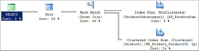
--Hash Match

 SELECT p.Name As ProductName, ps.Name As ProductSubcategoryName
 FROM Production.Product p
 JOIN Production.ProductSubcategory ps
   ON p.ProductSubcategoryID = ps.ProductSubcategoryID
 ORDER BY p.Name,  ps.Name
As discussed earlier, the hash join first scans or computes the entire build input and then builds a hash table in memory if it fits the memory grant. (In Figure 14-27, it is the Production.ProductSubCategory table.) Each row is inserted into a hash bucket according to the hash value computed for the hash key, so building the hash table needs memory. If the entire build input is smaller than the available memory, all rows can be inserted into the hash table. (You see what happens if there is not enough memory shortly.) This build phase is followed by the probe phase. The entire probe input (refer to Figure 14-27; it is the Production.Product table) is scanned or computed one row at a time, and for each probe row (from the Production.Product table), the hash key’s value is computed, the corresponding hash bucket (the one created from the Production.ProductSubCategory table) is scanned, and the matches are produced. This strategy is called an in-memory hash join.
If you’re talking about the AdventureWorks database running on your laptop with 1GB of RAM, you won’t have the problem of not fitting the hash table in memory. In the real world, however, with millions of rows in a table, there might not be enough memory to fit the hash table. If the build input does not fit in memory, a hash join proceeds in several steps. This is known as a grace hash join. In this hash join strategy, each step has a build phase and a probe phase. Initially, the entire build and probe inputs are consumed and partitioned (using a hash function on the hash keys) into multiple files. Using the hash function on the hash keys guarantees that any two joining records must be in the same pair of files. Therefore, the task of joining two large inputs has been reduced to multiple, but smaller, instances of the same tasks. The hash join is then applied to each pair of partitioned files. If the input is so large that the preceding steps need to be performed many times, multiple partitioning steps and multiple partitioning levels are required. This hash strategy is called a recursive hash join.
SQL Server always starts with an in-memory hash join and changes to other strategies if necessary.
Recursive hash joins (or hash bailouts) cause reduced performance in your server. If you see many Hash Warning events in a trace (the Hash Warning event is under the Errors and Warnings event class), update statistics on the columns that are being joined. You should capture this event if you see that you have many hash joins in your query. This ensures that hash bailouts are not causing performance problems on your server. When appropriate indexes on join columns are missing, the optimizer normally chooses the hash join.
Merge Join
The merge join, exemplified in the following code, relies on sorted input and is an efficient algorithm if both inputs are available sorted (see Figure 14-28).
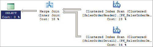
With a one-to-many merge join, a merge join operator scans each input only once, which is why it is superior to other operators if the predicate is not selective. For sorted input, the optimizer can use a clustered index. If a non-clustered index covers the join and select columns, the optimizer can choose that option because it has fewer pages to fetch.
A many-to-many merge join is a little more complicated. A many-to-many merge join uses a temporary table to store rows. If duplicate values exist from each input, one of the inputs must rewind to the start of the duplicates as each duplicate from the other input is processed.
In this query, both tables have a clustered index on the SalesOrderID column, so the optimizer chooses a merge join. Sometimes the optimizer chooses the merge join, even if one of the inputs is not presorted by an index, by adding a sort to the plan. The optimizer would do that if the input were small. If the optimizer chooses to sort before the merge, check whether the input has many rows and is not presorted by an index. To prevent the sort, you must add the required indexes to avoid a costly operation.
SELECT oh.SalesOrderID, oh.OrderDate,od.ProductID
 FROM Sales.SalesOrderDetail od
 JOIN Sales.SalesOrderHeader oh
   ON oh.SalesOrderID = od.SalesOrderID
Data Modification Query Plan
When you execute data modifications, the generated plan has two stages. The first stage is read-only, which determines which rows need to be inserted, updated, or deleted.
During the first stage, the execution plan generates a data stream that describes the changes. For INSERT statements you have column values, so the data stream contains the column values. DELETE statements have key column(s), and UPDATE statements have both data streams, the changed columns’ values and the table key. If you have foreign keys, the plan includes performing constraint validation. It also maintains indexes; and if any triggers exist, it fires these triggers as well.
The two maintenance strategies for INSERT, UPDATE, and DELETE statements are per-row and per-index. Consider the following DELETE query, which has a per-row query plan:
 DELETE FROM New_SalesOrderHeader
 WHERE OrderDate = '2007-07-01 00:00:00.000'
The query plan is shown in Figure 13-29.
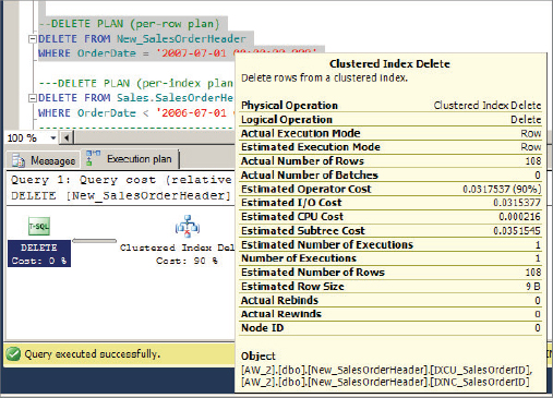
With a per-row plan, SQL Server 2012 maintains the indexes and the base table together for each row affected by the query. The updates to all non-clustered indexes are performed with each row update on the base table. The base table could be a heap or a clustered index. If you look at the Clustered Index Delete information box in Figure 13-29, in the Object information you can notice that both the clustered index and the non-clustered index are listed, which indicates that the indexes are maintained with a per-row operation.
Because of the short code path and update to all indexes and tables together, the per-row update strategy is more efficient in terms of CPU cycles.
Now consider another query plan with the following query. The change in this query is to the WHERE clause (changed to <). Use the Sales.SalesOrderHeader table to produce the plan for this example:
 DELETE FROM Sales.SalesOrderHeader
 WHERE OrderDate < '2006-07-01 00:00:00.000'
The query plan is shown in Figure 13-30. This figure shows only part of the plan because so many indexes are on this table in the AdventureWorks database. Run the statement in SSMS to see the full query plan.

This query plan performs per-index maintenance. The plan first deletes qualifying rows from the clustered index, and at the same time it builds the temporary spool table containing the clustering key values for the other non-clustered indexes that must be maintained. SQL Server 2012 reads the spool data as many times as the number of non-clustered indexes on the table. The sort operator between the index delete operator and the spool operator indicates that SQL Server 2012 sorts the data according to the key column of the index it is about to delete so that the index pages can be accessed optimally. The sequence operator enforces the execution order of each branch. SQL Server 2012 updates the indexes one after another from the top of the plan to the bottom.
As shown in the query plan, per-index maintenance is more complicated; but because it maintains individual indexes after sorting the key (Sort operator), it never visits the same page again, saving in I/O. Therefore, when you update many rows, the optimizer usually chooses the per-index plan.
Query Processing Enhancements on Partitioned Tables and Indexes
Before you look further into this topic, you may want to refer to the section “Partition Tables and Indexes” in Chapter 15 for a better understanding of partitioned tables.
SQL Server 2012 improves query processing performance on partitioned tables for many parallel plans, changing the way parallel and serial plans are represented. It also enhances the partitioning information provided in both compile-time and run-time execution plans to help you better understand what’s going on in the query plan.
Partitioned tables and indexes are supported only in SQL Server Enterprise and Developer editions.
Partition-Aware Seek Operation
The partition-aware SEEK operation is best understood through an example. Suppose you have a table called Sales with columns WeekID, GeographyID, ProductID, and SalesAmount. This table is partitioned on WeekID, which means each partition contains sales for a week. Suppose also that this table has a clustered index on GeographyID. Now say you want to perform a query like the following:
SELECT * FROM Sales WHERE GeographyID = 4 AND WeekID < 10
The partition boundaries for table Sales are defined by the following partition function:
CREATE PARTITION FUNCTION myRangePF1 (int) AS RANGE LEFT FOR VALUES (3, 7, 10);
In SQL Server 2012, when the query optimizer starts processing this query, it inserts PartitionID (which is hidden to represent the partition number in a partitioned table) as a leading column in the SEEK or SCAN operation. The query optimizer looks at the clustered index on GeographyID with composite columns, with PartitionID as the leading column (PartitionID, GeographyID). First, SQL Server 2012 determines which partitions it needs to look at during the first-level SEEK operation. In this case, because this table is partitioned on WeekID, and the predicate in the query is WeekID < 10, SQL Server 2012 can find all the partitions that have WeekID less than 10 first (see Figure 13-31). Here SQL Server 2012 finds three partitions that have WeekID less than 10, so it performs a second-level SEEK operation within those three partitions to find the records that have GeographyID = 4.

Parallel Query Execution Strategy for Partitioned Objects
SQL Server 2012 has implemented a new way to use parallelism to improve query performance when you access the partitioned table. If the number of threads is less than the number of partitions, the query processor assigns each thread to a different partition, initially leaving one or more partitions without an assigned thread. When a thread finishes executing on a partition, the query processor assigns it to the next partition until each partition has been assigned a single thread. This is the only case in which the query processor reallocates threads to other partitions.
If the number of threads is equal to the number of partitions, the query processor assigns one thread to each partition. When a thread finishes, it is not reallocated to another partition.
What if SQL Server 2012 has more threads than the number of partitions it actually needs to access to get the data? Refer to Figure 13-31. You have data in three partitions, and SQL Server has 10 threads to access the partitions. SQL Server uses all the available threads to access those partitions, but how can it assign those threads to each partition? It assigns three threads to each partition, and the remaining thread is assigned to one partition. Therefore, out of three partitions, two have six threads working on them (three threads each), and one partition has four threads working on it. If you have only one partition to access, then all the available threads are assigned to that partition — in this case, 10. When a thread finishes its execution, it is not reassigned to another partition.
Remember the following key points to achieve better query performance on partitioned tables when you access large amounts of data:
- Use more memory to reduce I/O cost if your performance data proves that your system is I/O bound.
- Take advantage that multicore processors are on a commodity server because SQL Server 2012 can also use it for parallel query processing capabilities.
- Make sure you have a clustered index on partitioned tables so that the query processor can take advantage of index scanning optimizations done in SQL Server 2012.
- If you aggregate a large amount of data from a partitioned table, make sure you have enough tempdb space on your server. See the article “Capacity Planning for tempdb” in BOL for more information on how to monitor tempdb space usage.
Execution Plans for Partitioned Heaps
As mentioned earlier, PartitionID is always a leading column to seek for a particular partition or range of partitions, even if the partitioned table is a heap. In SQL Server 2012, a partitioned heap is treated as a logical index on the partition ID. Partition elimination on a partitioned heap is represented in an execution plan as a Table Scan operator with a SEEK predicate on partition ID. The following example shows the Showplan information provided:
 |-- Table Scan (OBJECT: ([db].[dbo].[Sales]),
    SEEK: ([PtnId1001]=[Expr1011]) ORDERED FORWARD)
As you can see, even if it looks like a table scan, it still seeks on PartitionID.
Gathering Query Plans for Analysis with SQL Trace
Earlier you examined the query plans with different option such as SET STATISTICS PROFILE ON and SET STATISTICS XML ON. This technique does not work when you want to gather the query plans in your production environment. You have to use SQL Trace to get the query plan for analysis. See Chapter 12 for details about how to create server-side traces and import the trace data into a database table. You should create a server-side trace to capture events. In addition, import the data into a database table for analysis, rather than in SQL Profiler because SQL Profiler doesn’t offer as many options to play with data.
Please make sure that you set filters for your criteria when you gather the data with a server-side trace because the file size can grow quickly. In addition, depending on whether you prefer a textual execution plan or XML, you can check one of the events Showplan Statistics Profile or Showplan XML Statistics Profile.
In this chapter you learned how to do Query parsing, compiling, and optimization are all key performance tuning strategies in SQL Server 2012. Additionally, knowing how to read the query plan is imperative. When you read the query plan (using STATISTICS PROFILE, for example) the most important columns you want to look at are Rows, Executes, and EstimatedRows. If you see a big discrepancy between Rows (the actual row count) and EstimatedRows, remove that small query from your main query and start your analysis there. Not every performance problem with a query stems from bad statistics or cardinality estimations. In the real world, where users are less experienced, most performance problems result from user errors (lack of indexes and such). Check the statistics on the columns in the JOIN and WHERE clauses.
Another important part of Performance tuning includes the various index access methods and join algorithms. Normally, I/O is the slowest process, so your goal in query tuning is to reduce the number of I/Os and balance the data modification operation (in an OLTP system), and for that knowledge of the index, access methods and join algorithms are vital. Tuning is not easy, but with patience and attention to details, you can get to the root of the problem. Of course, make sure that your server and disk configuration are done properly. New features starting in SQL Server 2008 help facilitate the performance tuning you will perform, such as the MERGE and the query-processing enhancements on partitioned tables and indexes. Now that you know about configuring your server, optimizing SQL Server, and tuning queries, you can move on to learn about indexing your database in the next chapter.