Chapter 12
Monitoring Your SQL Server
WHAT’S IN THIS CHAPTER
- Monitor SQL Server Behavior with Dynamic Management
- Monitor SQL Server Error Log, and the Windows Event Logs
- A Quick Look at the Management Data Warehouse, UMDW, and Utility Control Point
- Monitoring SQL with the SCOM Management Pack, SQL Server Best Practices Analyzer, and System Center Advisor
Implementing good monitoring enables you to move from reactively dealing with events to proactively diagnosing problems and fixing them before your users are even aware there is a problem. This chapter teaches you how to proactively monitor your SQL Server system so that you can prevent or react to events before the server gets to the point where users begin calling.
Here’s a quick example. Say you recently took over an existing system after the DBA moved to a different team. This system’s applications ran well, but there was something that needed fixing every other day — transaction logs filling, tempdb out of space, not enough locks, and filegroups filling up; Nothing major, just a slow steady trickle of problems that needed fixing. This is the DBA’s death of 1,000 cuts. Your time is sucked away doing these essential maintenance tasks until you get to the point where you don’t have time to do anything else.
After a few weeks of this, you manage to put some new monitoring in place and make several proactive changes to resolve issues before anything breaks. These changes aren’t rocket science; they are simple things such as moving data to a new filegroup, turning on autogrow for several files and extending them to allow a known amount of growth, and rebuilding badly fragmented indexes that were reserving unneeded space. All this takes considerably less time than dealing with the steady stream of failures and provided a greatly improved experience for the users of this system.
So what does it take to monitor this system? Nothing dramatic — just a few simple steps, mostly some T-SQL monitoring of tables, database and filegroup free space, index usage, and fragmentation. I did a few things to monitor resource usage and help find the key pain points. After you understood the pain points, you can take a few steps to get ahead of the curve on fixing things.
Now that you’ve seen the value in monitoring SQL Server, you can learn how to do this for yourself.
The goal when monitoring databases is to see what’s going on inside SQL Server — namely, how effectively SQL Server uses the server resources (CPU, Memory, and I/O). You want this information so that you can see how well the system performs. The data needs to be captured over time to enable you to build a profile of what the system normally looks like: How much of what resource do you use for each part of the system’s working cycle? From the data collected over time you can start to build a baseline of “normal” activity. That baseline enables you to identify abnormal activities that might lead to issues if left unchecked.
Abnormal activity could be an increase in a specific table’s growth rate, a change in replication throughput, or a query or job taking longer than usual or using more of a scarce server resource than you expected. Identifying these anomalies before they become an issue that causes your users to call and complain makes for a much easier life. Using this data, you can identify what might be about to break, or where changes need to be made to rectify the root cause before the problem becomes entrenched.
Sometimes this monitoring is related to performance issues such as slow-running queries or deadlocks, but in many cases the data points to something that you can change to avoid problems in the future.
This philosophy is about the equivalent of “an apple a day keeps the doctor away” — preventative medicine for your SQL Server.
Determining Your Monitoring Objectives
Before you start monitoring you must first clearly identify your reasons for monitoring. These reasons may include the following:
- Establish a baseline.
- Identify new trends before they become problems.
- Monitor database growth.
- Identify daily, weekly, and monthly maintenance tasks.
- Identify performance changes over time.
- Audit user activity.
- Diagnose a specific performance problem.
Establishing a Baseline
Monitoring is extremely important to help ensure the smooth running of your SQL Server systems. However, just monitoring by itself, and determining the value of a key performance metric at any point in time, is not of great value unless you have a sound baseline to compare the metric against. Are 50 transactions per second good, mediocre, or bad? If the server runs at 75 percent CPU, is that normal? Is it normal for this time of day, on this day of the week, during this month of the year? With a baseline of the system’s performance, you immediately have something to compare the current metrics against.
If your baseline shows that you normally get 30 transactions per second, then 50 transactions per second might be good; the system can process more transactions. However, it may also be an indication that something else is going on, which has caused an increase in the transactions. What your baseline looks like depends on your system, of course. In some cases it might be a set of Performance Monitor logs with key server resource and SQL counters captured during several periods of significant system activity, or stress tests. In another case, it might be the results of analysis of a SQL Profiler trace captured during a period of high activity. The analysis might be as simple as a list of the stored procedure calls made by a particular application, with the call frequency.
To determine whether your SQL Server system performs optimally, take performance measurements at a regular interval over time, even when no problem occurs, to establish a server performance baseline. How many samples and how long each needs to be are determined by the nature of the workload on your servers. If your servers have a cyclical workload, the samples should aim to query at multiple points in several cycles to allow a good estimation of min, max, and average rates. If the workload is uniform, then fewer samples over shorter periods can provide a good indication of min, max, and average rates. At a minimum, use baseline performance to determine the following:
- Peak and off-peak hours of operation
- Query or batch response time
Another consideration is how often the baseline should be recaptured. In a system that is rapidly growing, you may need to recapture a baseline frequently. When current performance has changed by 15 to 25 percent compared to the old baseline, it is a good point to consider recapturing the baseline.
Comparing Current Metrics to the Baseline
A key part of comparing current metrics to those in the baseline is determining an acceptable limit from the baseline outside of which the current metric is not acceptable and which flags an issue that needs investigating.
What is acceptable here depends on the application and the specific metric. For example, a metric looking at free space in a database filegroup for a system with massive data growth and an aggressive archiving strategy might set a limit of 20 percent free space before triggering some kind of alert. On a different system with little database growth, that same metric might be set to just 5 percent.
You must make your own judgment of what is an acceptable limit for deviation from the baseline based on your knowledge of how your system is growing and changing.
CHOOSING THE APPROPRIATE MONITORING TOOLS
After you define your monitoring goals, you should select the appropriate tools for monitoring. The following list describes the basic monitoring tools:
- Performance Monitor: Performance Monitor is a useful tool that tracks resource use on Microsoft operating systems. It can monitor resource usage for the server and provide information specific to SQL Server either locally or for a remote server. You can use it to capture a baseline of server resource usage, or it can monitor over longer periods of time to help identify trends. It can also be useful for ad hoc monitoring to help identify any resource bottlenecks responsible for performance issues. You can configure it to generate alerts when predetermined thresholds are exceeded.
- Extended Events: Extended Events provide a highly scalable and configurable architecture to enable you to collect information to troubleshoot issues with SQL Server. It is a lightweight system with a graphical UI that enables new sessions to be easily created.
Extended Events provides the system_health session. This is a default health session that runs with minimal overhead, and continuously collects system data that may help you troubleshoot your performance problem without having to create your own custom Extended Events session.
While exploring the Extended Events node in SSMS, you may notice an additional default session, the AlwaysOn_health session. This is an undocumented session created to provide health monitoring for Availability Groups.
- SQL Profiler: This tool is a graphical application that enables you to capture a trace of events that occurred in SQL Server. All SQL Server events can be captured by this tool into the trace. The trace can be stored in a file or written to a SQL Server table.
SQL Profiler also enables the captured events to be replayed. This makes it a valuable tool for workload analysis, testing, and performance tuning. It can monitor a SQL Server instance locally or remotely. You can also use the features of SQL Profiler within a custom application, by using the Profiler system stored procedures.
SQL Profiler has been deprecated in SQL Server 2012, so you should plan on moving away from using this tool, and instead use Extended events for trace capture activities, and Distributed Replay for replaying events.
- SQL Trace: SQL Trace is the T-SQL stored procedure way to invoke a SQL Server trace without needing to start up the SQL Profiler application. It requires a little more work to set up, but it’s a lightweight way to capture a trace; and because it’s scriptable, it enables the automation of trace capture, making it easy to repeatedly capture the same events.
With the announcement of the deprecation of SQL Server profiler, you should start moving all your trace based monitoring to Extended Events.
- Default trace: Introduced with SQL Server 2005, the default trace is a lightweight trace that runs in a continuous loop and captures a small set of key database and server events. This is useful in diagnosing events that may have occurred when no other monitoring was in place.
- Activity Monitor in SQL Server Management Studio: This tool graphically displays the following information:
- Processes running on an instance of SQL Server
- Resource Waits
- Data File IO activity
- Recent Expensive Queries
- Dynamic management views and functions: Dynamic management views and functions return server state information that you can use to monitor the health of a server instance, diagnose problems, and tune performance. These are one of the best tools added to SQL Server 2005 for ad hoc monitoring. These views provide a snapshot of the exact state of SQL Server at the point they are queried. This is extremely valuable, but you may need to do a lot of work to interpret the meaning of some of the data returned, because they often provide just a running total of some internal counter. You need to add quite a bit of additional code to provide useful trend information. There are numerous examples in the “Monitoring with Dynamic Management Views and Functions” section later in this chapter that show how to do this.
- System Stored procedures: Some system-stored procedures provide useful information for SQL Server monitoring, such as sp_who, sp_who2, sp_lock, and several others. These stored procedures are best for ad hoc monitoring, not trend analysis.
- Utility Control Point (UCP): The Utility Control Point is a management construct introduced in SQL Server 2008 R2. It adds to the Data Collection sets of the Management Data Warehouse and includes reports on activity within a SQL Server Utility. The SQL Server Utility is another addition for SQL Server 2008 R2, and is a management container for server resources that can be monitored using the UCP.
- Standard Reports: The standard reports that ship with SQL Server are a great way to get a look into what’s happening inside SQL Server without needing to dive into DMVs, Extended Events, and the default Trace.
- SQL Server Best Practice Analyzer: A set of rules implemented in Microsoft Baseline Configuration Analyzer (MBCA) that implement checks for SQL Server best practices. The tool is available as a download, and has a fixed set of rules. Also see System Center Advisor.
- System Center Advisor: An extension of the SQL Server Best Practice Analyzer, this is a cloud-based utility to analyze your SQL Servers and provide feedback on their configuration and operation against the set of accepted best practices for configuring and operating SQL Server.
- System Center Management Pack: SQL Server has had a management pack for some time now, but it’s not well known, or used by DBAs. The Management Pack enables you to create exception-driven events that drive operator interaction with SQL Server to resolve specific issues. The rest of the chapter discusses these tools in detail.
Performance Monitor, also known as Perfmon, or System Monitor, is the User Interface that most readers will become familiar with as their interface with Performance Monitoring. Performance Monitor is a Windows tool that’s found in the Administrative Tools folder on any Windows PC, or Server. It has the ability to graphically show performance counter data as a graph (the default setting) or as a histogram, or in a textual report format.
Performance Monitor is an important tool because not only does it inform you about how SQL Server performs, it is also the tool that indicates how Windows performs. Performance Monitor provides a huge set of counters, but don’t be daunted. This section covers a few of them, but there is likely no one who understands all of them.
This section is not an introduction to using Performance Monitor. (Although later in this section you learn about two valuable tools, Logman, and Relog, that make using Performance Monitor a lot easier in a production environment.) This section instead focuses on how you can use the capabilities of this tool to diagnose performance problems in your system. For general information about using Performance Monitor, look at the Windows 7 or Windows Server 2008 R2 documentation.
As mentioned in the previous section “The Goal of Monitoring,” you need to monitor three server resources:
- CPU
- Memory
- I/O (primarily disk I/O)
Monitor these key counters over a “typical” interesting business usage period. Depending on your business usage cycles, this could be a particular day, or couple of days when the system experiences peaks of usage. You would not gather data over a weekend or holiday. You want to get an accurate picture of what’s happening during typical business usage, and not when the system is idle. You should also take into account any specific knowledge of your business and monitor for peaks of activity such as end of week, end of month, or other special activities.
DETERMINING SAMPLE TIME
The question of what sample period to use often comes up. (Sample period is displayed as the “Sample Every” value on the general tab of a Performance Monitor chart’s property page.) A general rule of thumb is that the shorter the overall monitoring period, then the shorter the sample period. If you are capturing data for 5-10 minutes you might use a one second sample interval. If you are capturing data for multiple days, then 15 seconds, 30 seconds, or even 1-5 minutes might be better sample periods. The real decision points are around managing the overall capture file size, and ensuring that the data you capture has fine enough resolution to let you discern interesting events. If you are looking for something that happens over a short period of time, then you need an even shorter sample time to be able to see it. So for an event that you think might last 10-15 seconds, you should aim for a sample rate that gives you at least 3-5 samples during that period; for the 15 second event, you might choose a 3 second sample period, which would give you 5 samples during the 15 second event. One last point to consider is that if you’re interested in maintenance activity performance, such as for backups, index maintenance, data archival, and so on, then that actually is a case where you might want to monitor at night and on weekends, and during normal business down time, as that’s when the maintenance activities are typically scheduled to run.
CPU Resource Counters
Several counters show the state of the available CPU resources. Bottlenecks due to CPU resource shortages are frequently caused by problems such as more users than expected, one or more users running expensive queries, or routine operational activities such as index rebuilding.
The first step to find the cause of the bottleneck is to identify that the bottleneck is a CPU resource issue. The following counters can help you do this:
- Object: Processor - Counter: % Processor Time: This counter determines the percentage of time each processor is busy. There is a _Total instance of the counter that for multiprocessor systems measures the total processor utilization across all processors in the system. On multiprocessor machines, the _Total instance might not show a processor bottleneck when one exists. This can happen when queries execute that run on either a single thread or fewer threads than there are processors. This is often the case on OLTP systems, or where MAXDOP has been set to less than the number of processors available.
In this case, a query can be bottlenecked on the CPU as it’s using 100 percent of the single CPU it’s scheduled to run on, or in the case of a parallel query as it’s using 100 percent of multiple CPUs, but in both cases other idle CPUs are available that this query is not using.
If the _Total instance of this counter is regularly at more than 80 percent, that’s a good indication that the server is reaching the limits of the current hardware. Your options here are to buy more or faster processors, or optimize the queries to use less CPU. See Chapter 11, “Optimizing SQL Server 2012,” for a detailed discussion on hardware.
- Object: System - Counter: Processor Queue Length: The processor queue length is a measure of how many threads sit in a ready state waiting on a processor to become available to run them. Interpreting and using this counter is an advanced operating system performance-tuning option needed only when investigating complex multithreaded code problems. For SQL Server systems, processor utilization can identify CPU bottlenecks much more easily than trying to interpret this counter.
- Object: Processor - Counter: % Privileged Time: This counter indicates the percentage of the sample interval when the processor was executing in kernel mode. On a SQL Server system, kernel mode time is time spent executing system services such as the memory manager, or more likely, the I/O manager. In most cases, privileged time equates to time spent reading and writing from disk or the network.
It is useful to monitor this counter when you find an indication of high CPU usage. If this counter indicates that more than 15 percent to 20 percent of processor time is spent executing privileged code, you may have a problem, possibly with one of the I/O drivers, or possibly with a filter driver installed by antivirus software scanning the SQL data or log files.
- Object: Process - Counter: % Processor Time - Instance: sqlservr: This counter measures the percentage of the sample interval during which the SQL Server Process uses the available processors. When the Processor % Processor Time counter is high, or you suspect a CPU bottleneck, look at this counter to confirm that it is SQL Server using the CPU, and not some other process.
- Object: Process - Counter: % Privileged Time - Instance: sqlservr: This counter measures the percentage of the sample that the SQL Server Process runs in kernel mode. This will be the kernel mode portion of the total %ProcessorTime shown in the previous counter. As with the previous counter, this counter is useful when investigating high CPU usage on the server to confirm that it is SQL Server using the processor resource, and not some other process.
- Object: Process - Counter: % User Time - Instance: sqlservr: This counter measures the percentage of the sample that the SQL Server Process runs in User mode. This is the User mode portion of the total %ProcessorTime shown in the previous counter. Combined with %Privileged, time should add up to %ProcessorTime.
After determining that you have a processor bottleneck, the next step is to track down its root cause. This might lead you to a single query, a set of queries, a set of users, an application, or an operational task causing the bottleneck. To further isolate the root cause, you need to dig deeper into what runs inside SQL Server. See the Performance Monitoring Tools section later in this chapter to help you do this. After you identify a processor bottleneck, consult the relevant chapter for details on how to resolve it. See Chapter 10 for information on “Configuring the Server for Optimal Performance,” Chapter 11 for “Optimizing SQL Server 2012,” Chapter 13 for “Performance Tuning T-SQL,” and Chapter 14 for information on “Indexing Your Database.”
Disk Activity
SQL Server relies on the Windows operating system to perform I/O operations. The disk system handles the storage and movement of data on your system, giving it a powerful influence on your system’s overall responsiveness. Disk I/O is frequently the cause of bottlenecks in a system. You need to observe many factors in determining the performance of the disk system, including the level of usage, the rate of throughput, the amount of disk space available, and whether a queue is developing for the disk systems. Unless your database fits into physical memory, SQL Server constantly brings database pages into and out of the buffer pool. This generates substantial I/O traffic. Similarly, log records need to be flushed to the disk before a transaction can be declared committed. SQL Server 2005 started to make considerably more use of tempdb and this hasn’t changed with SQL Server 2012, so beginning with SQL Server 2005, tempdb I/O activity can also cause a performance bottleneck.
Many of the disk I/O factors are interrelated. For example, if disk utilization is high, disk throughput might peak, latency for each I/O starts to increase, and eventually a queue might begin to form. These conditions can result in increased response time, causing performance to slow.
Several other factors can impact I/O performance, such as fragmentation or low disk space. Make sure you monitor for free disk space and take action when it falls below a given threshold. In general, the level of free space to raise an alert is when free disk space falls below 15 percent to 20 percent. Above this level of free space, many disk systems start to slow down because they need to spend more time searching for increasingly fragmented free space.
You should look at several key metrics when monitoring I/O performance:
- Throughput, IOPS: How many I/Os per second (IOPS) can the storage subsystem deliver?
- Throughput, MB/sec: How many MB/sec can the I/O subsystem deliver?
- Latency: How long does each I/O request take?
- Queue depth: How many I/O requests are waiting in the queue?
For each of these metrics you should also distinguish between read-and-write activity.
Physical Versus Logical Disk Counters
There is often confusion around the difference between Physical and Logical Disk Counters. This section explains the similarities and differences, provides specific examples of different disk configurations, and explains how to interpret the results seen on the different disk configurations.
One way to think about the difference between the logical and the physical disk counters is that the logical disk counters monitor I/O where the I/O request leaves the application layer (or as the requests enter kernel mode), whereas the physical disk counters monitor I/O as it leaves the bottom of the kernel storage driver stack. Figure 12-1 shows the I/O software stack and illustrates where the logical disk and physical disk counters monitor I/O.

In some scenarios the logical and physical counters provide the same results; in others they provide different results.
The different IO subsystem configurations that affect the values displayed by the logical and physical disk counters are discussed in the following sections.
Single Disk, Single Partition
Figure 12-2 shows a single disk with a single partition. In this case there will be a single set of logical disk counters and a single set of physical disk counters. This configuration works well in a small SQL Server configuration with a few disks, where the SQL data and log files are already spread over multiple Single Disk, Single Partition disks.

Single Disk, Multiple Partitions
Figure 12-3 shows a single disk split into multiple partitions. In this case, there are multiple instances of the logical disk counters, one per partition, and just a single set of physical disk counters. This kind of configuration doesn’t provide any performance advantages, but it does allow more accurate monitoring of I/O to the different partitions. If you place different sets of data onto different partitions, you can see how much I/O goes to each set by monitoring the logical disk counters.

One danger with this configuration is that you may be mislead into thinking you actually have different physical disks, and so you think you are isolating data IO from Log IO from tempdb IO because they are on different “drives,” when in fact, all the IO is going to the same physical disk.
An example of this might be to put SQL log files on one partition, tempdb data files on another partition, a filegroup for data on another partition, a filegroup for indexes on another partition, and backups on another partition.
Multiple Disks, Single Volume — Software RAID
Figure 12-4 shows multiple disks configured in a software RAID array and mounted as a single volume. In this configuration there is a single set of logical disk counters and multiple sets of physical disk counters.

This configuration works well in a small SQL Server configuration where the hardware budget won’t stretch to a RAID array controller, but multiple disks are available and you want to create a RAID volume spanning them. For more information on RAID, refer to Chapter 10, “Configuring the Server for Optimal Performance.”
Multiple Disks, Single Volume — Hardware RAID
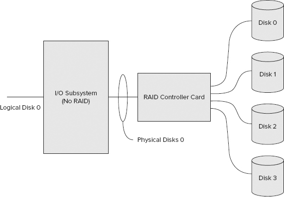
Figure 12-5 shows a hardware RAID array. In this configuration, multiple disks are managed by the hardware RAID controller. The operating system sees only a single physical disk presented to it by the array controller card. The disk counters appear to be the same as the single disk, single partition configuration — that is, a single set of physical disk counters and a corresponding single set of logical disk counters.
The Object: Physical Disk - Counter: Disk Writes/Sec and Object: Physical Disk - Counter: Disk Reads/Sec provide information about how many I/O operations are performed per second over the sample interval. This information is useful to determine whether the I/O subsystem is approaching capacity. It can be used in isolation to compare against the theoretical ideal for the I/O subsystem based upon the number and type of disks in the I/O subsystem. It is also useful when compared against the I/O subsystem baseline to determine how close you are to maximum capacity.
Monitoring I/O Throughput - MB/Sec
The Object: Physical Disk - Counter: Disk Write Bytes/Sec and Object: Physical Disk - Counter: Disk Read Bytes/Sec provide information about how many MB/Sec are read and written to and from the disk over the sample interval. This is an average over the sample period, so with long sample periods it may average out to big peaks and troughs in throughput. Over a short sample period, this may fluctuate dramatically, as it sees the results of one or two larger I/Os flooding the I/O subsystem. This information is useful to determine whether the I/O subsystem is approaching its capacity.
As with the other Disk IO counters, Disk Read Bytes/Sec and Disk Write Bytes/Sec can be used in isolation to compare against the theoretical throughput for the number and type of disks in the I/O subsystem, but it is more useful when it can be compared against a baseline of the maximum throughput available from the I/O subsystem.
Monitoring I/O Latency
The Object: Physical Disk - Counter: Avg. Disk Sec/Write and Object: Physical Disk - Counter: Avg. Disk Sec/Read provide information on how long each read-and-write operation is taking. These two counters show average latency. It is an average taken over every I/O issued during the sample period.
This information is extremely useful and can be used independently to determine how well the I/O subsystem deals with the current I/O load. Ideally, these counters should be below 5–10 milliseconds (ms). On larger data warehouse or decision support systems, it is acceptable for the values of these counters to be in the range of 10–20 ms. Sustained values over 50 ms are an indication that the I/O subsystem is heavily stressed, and that a more detailed investigation of I/O should be undertaken.
These counters show performance degradations before queuing starts. These counters should also be used with the following disk queue length counters to help diagnose I/O subsystem bottlenecks.
Monitoring I/O Queue Depth
The Object: Physical Disk - Counter: Avg. Disk Write Queue Length and Object: Physical Disk - Counter: Avg. Disk Read Queue Length provide information on the read-and-write queue depth. These two counters show the average queue depth over the sample period. Disk queue lengths greater than 2 for a single physical disk indicate that there may be an I/O subsystem bottleneck.
Correctly interpreting these counters is more challenging when the I/O subsystem is a RAID array, or when the disk controller has built-in caching and intelligence. In these cases, the controller will have its own queue, which is designed to absorb and buffer, and effectively hide from this counter, any queuing going on at the disk level. For these reasons, monitoring these counters is less useful than monitoring the latency counters. If these counters do show queue lengths consistently greater than 2, it’s a good indication of a potential I/O subsystem bottleneck.
Monitoring Individual Instances Versus Total
In multidisk systems with several disks, monitoring all the preceding counters for all available disks provides a mass of fluctuating counters to monitor. In some cases, monitoring the _Total instance, which combines the values for all instances, can be a useful way to detect I/O problems. The scenario in which this doesn’t work is when I/O to different disks has different characteristics. In this case, the _Total instance shows a reasonably good average number, although some disks may sit idle and others melt from all the I/O requests they service.
Monitoring Transfers Versus Read and Write
One thing you may have noticed in the list of counters is that the transfer counters are missing. This is because the transfer counters average out the read-and-write activity. For a system that is heavy on one kind of I/O at the expense of the other (reads versus writes), the transfer counters do not show an accurate picture of what happens.
In addition, read I/O and write I/O usually have different characteristics, and different performance than the underlying storage. Monitoring a combination of two potentially disparate values doesn’t provide a meaningful metric.
Monitoring %Disk Counters
Another set of disk counters missing from this list are all the %Disk counters. Although these counters can provide interesting information, there are enough problems with the results (that is, the total percentage can often exceed 100) that these counters don’t provide a useful detailed metric.
If you can afford to monitor all the counters detailed in the preceding sections, you can have a much more complete view of what’s going on with your system.
If you want a few simple metrics that provide a good approximate indication of overall I/O subsystem activity, then the %Disk Time, %Disk Read Time, and %Disk Write time counters can provide that.
Isolating Disk Activity Created by SQL Server
All the counters you should monitor to find disk bottlenecks have been discussed. However, you may have multiple applications running on your servers, and one of those other applications could cause a lot of disk I/O. To confirm that the disk bottleneck is being caused by SQL Server, you should isolate the disk activities created by SQL Server. Monitor the following counters to determine whether the disk activity is caused by SQL server:
- SQL Server: Buffer Manager: Page reads/sec
- SQL Server: Buffer Manager: Page writes/sec
Sometimes your application is too big for the hardware you have, and a problem that appears to be related to disk I/O may be resolved by adding more RAM. Make sure you do a proper analysis before making a decision. That’s where trend analysis is helpful because you can see how the performance problem evolved.
Is Disk Performance the Bottleneck?
With the help of the disk counters, you can determine whether you have disk bottlenecks in your system. Several conditions must exist for you to make that determination, including a sustained rate of disk activity well above your baseline, persistent disk queue length longer than two per disk, and the absence of a significant amount of paging. Without this combination of factors, it is unlikely that you have a disk bottleneck in your system.
Sometimes your disk hardware may be faulty, and that could cause a lot of interrupts to the CPU. Another possibility could be that a processor bottleneck is caused by a disk subsystem, which can have a systemwide performance impact. Make sure you consider this when you analyze the performance data.
If, after monitoring your system, you come to the conclusion that you have a disk bottleneck, you need to resolve the problem. See Chapter 10, for more details on configuring SQL Server for optimal performance, Chapter 11 for optimizing SQL Server, and Chapter 13, “Performance Tuning T-SQL” for SQL query tuning.
Memory Usage
Memory is perhaps the most critical resource affecting SQL Server performance. Without enough memory, SQL Server is forced to keep reading and writing data to disk to complete a query. Disk access is anywhere from 1,000 to 100,000 times slower than memory access, depending on exactly how fast your memory is.
Because of this, ensuring SQL Server has enough memory is one of the most important steps you can take to keep SQL Server running as fast as possible. Monitoring memory usage, how much is available, and how well SQL Server uses the available memory is therefore a vitally important step.
In an ideal environment, SQL Server runs on a dedicated machine and shares memory only with the operating system and other essential applications. However, in many environments, budget or other constraints mean that SQL shares a server with other applications. In this case you need to monitor how much memory each application uses and verify that everyone plays well together.
Low memory conditions can slow the operation of the applications and services on your system. Monitor an instance of SQL Server periodically to confirm that the memory usage is within typical ranges. When your server is low on memory, paging — the process of moving virtual memory back and forth between physical memory and the disk — can be prolonged, resulting in more work for your disks. The paging activity might need to compete with other transactions performed, intensifying disk bottleneck.
Since SQL Server is one of the best behaved server applications available, when the operating system triggers the low memory notification event, SQL releases memory for other applications to use; it actually starves itself of memory if another memory-greedy application runs on the machine. The good news is that SQL releases only a small amount of memory at a time, so it may take hours, and even days, before SQL starts to suffer. Unfortunately, if the other application desperately needs more memory, it can take hours before SQL frees up enough memory for the other application to run without excessive paging. Since issues such as those mentioned can cause significant problems, monitor the counters described in the following sections to identify memory bottlenecks.
Solid State Drives (SSD) are starting to appear at lower cost points that make them attractive for use in more database configurations. Although the I/O throughput of SSDs is 100s to 1000s of times larger and faster than even the fastest spinning disks, their throughput is still considerably lower, and their latency higher than direct memory access. However, it is still too soon to determine how the slow march of solid state devices can alter how you think about memory usage in SQL Server.
Monitoring Available Memory
The Object: Memory - Counter: Available Mbytes reports how many megabytes of memory are currently available for programs to use. It is the best single indication that there may be a memory bottleneck on the server.
Determining the appropriate value for this counter depends on the size of the system you monitor. If this counter routinely shows values less than 128MB, you may have a serious memory shortage.
On a server with 4GB or more of physical memory (RAM), the operating system can send a low memory notification when available memory reaches 128MB. At this point, SQL releases some of its memory for other processes to use.
Ideally, aim to have at least 256MB to 500MB of Available MBytes. On larger systems with more than 16GB of RAM, this number should be increased to 500MB–1GB. If you have more than 64GB of RAM on your server, increase this to 1–2GB.
Monitoring SQL Server Process Memory Usage
Having used the Memory – Counter: Available Mbytes to determine that a potential memory shortage exists; the next step is to determine which processes use the available memory. As your focus is on SQL Server, you hope that it is SQL Server that uses the memory. However, you should always confirm that this is the case.
The usual place to look for a process’s memory usage is in the Process object under the instance for the process. For SQL Server, these counters are detailed in the following list:
- Object: Process – Instance: sqlserver - Counter: Virtual Bytes: This counter indicates the size of the virtual address space allocated by the process. Virtual address space (VAS) is used by a lot of processes that aren’t related to memory performance. This counter is of value when looking for the root cause of SQL Server out-of-memory errors. If running on a 32-bit system, virtual address space is limited to 2GB (except when the /3GB switch is enabled). In this environment, if virtual bytes approach 1.5GB to 1.7GB, that is about as much space as can be allocated. At this point the root cause of the problem is a VAS limitation issue, and the resolution is to reduce SQL Server’s memory usage, enable AWE, boot using /3GB, or move to a 64-bit environment. On a 64-bit system this counter is of less interest because VAS pressure is not going to occur. To learn more about AWE, refer to Chapter 11.
This counter includes the AWE window, but it does not show how much physical memory is reserved though AWE.
- Object: Process – Instance: sqlservr – Counter: Working Set: This counter indicates the size of the working set for the SQL Server process. The working set is the total set of pages currently resident in memory, as opposed to being paged to disk. It can provide an indication of memory pressure when this is significantly lower than the Private Bytes for the process.
This counter does not include AWE memory allocations.
- Object: Process – Instance: sqlservr – Counter: Private Bytes: The Private Bytes counter tells you how much memory this process has allocated that cannot be shared with other processes — that is, it’s private to this process. To understand the difference between this counter and virtual bytes, you just need to know that certain files loaded into a process’s memory space — the EXE, any DLLs, and memory mapped files — will automatically be shared by the operating system. Therefore, Private Bytes indicates the amount of memory used by the process for its stacks, heaps, and any other virtually allocated memory in use. You could compare this to the total memory used by the system. When this value is a significant portion of the total system memory, it is a good indication that SQL Server memory usage is the root of the overall server memory shortage.
It does not show anything about AWE memory.
Monitoring SQL Server AWE Memory
In SQL Server 2012, support for using AWE on 32-bit systems has been removed, so this section is only relevant to 64-bit systems.
If your SQL Server is configured to use AWE memory, the regular process memory counters do not show how much memory SQL Server actually uses. In this scenario, you may see “AvailableMB,” indicating that 15GB of the available 16GB of memory is in use, but when you add up the memory actually in use (the working set) for all running processes, it falls a long way short of the 15GB used. This is because SQL Server has taken 12GB of memory and uses it through AWE.
In this case, the only way to see this AWE memory is to look at the SQL Server–specific counters that indicate how much memory SQL uses:
- Object: SQL Server:Buffer Manager – Counter: Database Pages: Shows the number of pages used by the buffer pool for database content
- Object: SQL Server:Buffer Manager – Counter; Target Pages: Shows how many pages SQL Server wants to allocate for the buffer pool
- Object: SQL Server:Buffer Manager – Counter: Total Pages: Shows how many pages SQL Server currently uses for the buffer pool
- Object: SQL Server:Memory Manager – Counter: Target Server Memory (KB): Shows how much memory SQL Server would like to use for all its memory requirements
- Object: SQL Server:Memory Manager – Counter: Total Server Memory (KB): Shows how much memory SQL Server currently uses
Other SQL Server Memory Counters
The following is a list of some additional SQL Server memory counters. When looking at memory issues, these counters can provide more detailed information than the counters already described:
- Buffer Cache Hit Ratio: This counter indicates how many page requests were found in the buffer pool. It tends to be a little coarse in that 98 percent and above is good, but 97.9 percent might indicate a memory issue.
- Free Pages: This counter indicates how many free pages SQL Server has for new page requests. Acceptable values for this counter depend on how much memory you have available and the memory usage profile for your applications. Having a good baseline is useful, as the values for this counter can be compared to the baseline to determine whether there is a current memory issue, or whether the value is part of the expected behavior of the system.
This counter should be read with the Page Life Expectancy counter.
- Page Life Expectancy: This counter provides an indication of the time, in seconds, that a page is expected to remain in the buffer pool before being flushed to disk. The current Best Practices from Microsoft state that values above 300 are generally considered okay. Values approaching 300 are a cause for concern. Values below 300 are a good indication of a memory shortage. These Best Practices are now getting a bit dated however. They were written when a large system might have 4 dual or quad core processors, and 16GB of RAM. Today’s commodity hardware comes with a 2P system with 10, 12, 16+ cores, and the ability to have 256GB or more of memory. Therefore, those best practice numbers are less relevant. Because of this, you should interpret this counter in conjunction with other counters to understand if there really is memory pressure.
Read this counter with the Free Pages counter. You should expect to see Free Pages drop dramatically as the page life expectancy drops below 300. When considered together, Free Pages and Page Life expectancy provide an indication of memory pressure that may result in a bottleneck.
Scripting Memory Counters with Logman
Following is a Logman script that can create a counter log of the memory counters discussed in this section (see the “Logman” section later in the chapter for more information):
Logman create counter "Memory Counters" -si 05 -v nnnnnn -o
"c:perflogsMemory Counters" -c "MemoryAvailable MBytes"
"Process(sqlservr)Virtual Bytes" "Process(sqlservr)Working Set"
"Process(sqlservr)Private Bytes" "SQLServer:Buffer ManagerDatabase
pages" "SQLServer:Buffer ManagerTarget pages" "SQLServer:Buffer
ManagerTotal pages" "SQLServer:Memory ManagerTarget Server Memory (KB)"
"SQLServer:Memory ManagerTotal Server Memory (KB)"
Resolving Memory Bottlenecks
The easy solution to memory bottlenecks is to add more memory; but previously stated, tuning your application always comes first. Try to find queries that are memory-intensive, for instance queries with large worktables — such as hashes for joins and sorts — to see if you can tune them. You can learn more about tuning T-SQL queries in Chapter 13 “Performance Tuning T-SQL.”
In addition, refer to Chapter 10 to ensure that you have configured your server properly. If you are running a 32-bit machine and after adding more memory you are still running into memory bottlenecks, then look into a 64-bit system.
Performance Monitoring Tools
A few tools are well hidden in the command-line utilities that have shipped with Windows operating systems for some time. Two of these that are extremely valuable when using Performance Monitor are Logman and Relog.
Logman
Logman is a command-line way to script performance monitoring counter logs. You can create, alter, start, and stop counter logs using Logman.
You have seen several examples earlier in this chapter of using Logman to create different counter logs. Following is a short command-line script file to start and stop a counter collection:
REM start counter collection
logman start "Memory Counters"
timeout /t 5
REM add a timeout for some short period
REM to allow the collection to start
REM do something interesting here

REM stop the counter collection
logman stop "Memory Counters"
timeout /t 5
REM make sure to wait 5 to ensure its stopped
Complete documentation for Logman is available through the Windows help system.
Logman Script for I/O Counters
The following script can create a new counter log called IO Counters and collect samples for every counter previously detailed, for all instances and with a 5-second sample interval, and write the log to c:perflogsIO Counters, appending a six-digit incrementing sequence number to each log:
Logman create counter "IO Counters" -si 05 -v nnnnnn -o "c:perflogsIO
Counters" -c "PhysicalDisk(*)Avg. Disk Bytes/Read" " PhysicalDisk(*)Avg.
Disk Bytes/Write" "PhysicalDisk(*)Avg. Disk Read Queue Length"
"PhysicalDisk(*)Avg. Disk sec/Read" "PhysicalDisk(*)Avg. Disk sec/Write"
"PhysicalDisk(*)Avg. Disk Write Queue Length" "PhysicalDisk(*)Disk Read
Bytes/sec" "PhysicalDisk(*)Disk Reads/sec" "PhysicalDisk(*)Disk Write
Bytes/sec" "PhysicalDisk(*)Disk Writes/sec"
After running this script, run the following command to confirm that the settings are as expected:
logman query "IO Counters"
Relog
Relog is a command-line utility that enables you to read a log file and write selected parts of it to a new log file.
You can use it to change the file format from blg to csv. You can use it to resample data and turn a large file with a short sample period into a smaller file with a longer sample period. You can also use it to extract a short period of data for a subset of counters from a much larger file.
Complete documentation for Relog is available through the Windows help system.
Events are fired at the time of some significant occurrence within SQL Server. Using events enables you to react to the behavior at the time it occurs, and not have to wait until some later time. SQL Server generates many different events and has several tools available to monitor some of these events.
The following list describes the different features you can use to monitor events that happened in the Database Engine:
- system_health Session: The system_health session is included by default with SQL Server, starts automatically when SQL Starts, and runs with no noticeable performance impact. It collects a minimal set of system information that can help resolve performance issues.
- Default Trace: Initially added in SQL Server 2005, this is perhaps one of the best kept secrets in SQL Server. It’s virtually impossible to find any documentation on this feature. The default trace is basically a flight data recorder for SQL Server. It records the last 5MB of key events. The events it records were selected to be lightweight, yet valuable when troubleshooting a critical SQL event.
- SQL Trace: This records specified events and stores them in a file (or files) that you can use later to analyze the data. You have to specify which Database Engine events you want to trace when you define the trace. Following are two ways to access the trace data:
- Using SQL Server Profiler, a graphical user interface
- Through T-SQL system stored procedures
- SQL Server Profiler: This exploits all the event-capturing functionality of SQL Trace and adds the capability to trace information to or from a table, save the trace definitions as templates, extract query plans and deadlock events as separate XML files, and replay trace results for diagnosis and optimization. Another option, and perhaps least understood, is using a database table to store the trace. Storing the trace file in a database table enables the use of T-SQL queries to perform complex analysis of the events in the trace.
- Event notifications: These send information to a Service Broker service about many of the events generated by SQL Server. Unlike traces, event notifications can be used to perform an action inside SQL Server in response to events. Because event notifications execute asynchronously, these actions do not consume any resources defined by the immediate transaction, meaning, for example, that if you want to be notified when a table is altered in a database, then the ALTER TABLE statement would not consume more resources or be delayed because you have defined event notification.
- Extended Events: These were new with SQL Server 2008 and extend the Event Notification mechanism. They are built on the Event Tracing for Windows (ETW) framework. Extended Events are a different set of events from those used by Event Notifications and can be used to diagnose issues such as low memory conditions, high CPU use, and deadlocks. The logs created when using SQL Server Extended Events can also be correlated with other ETW logs using tracerpt.exe. See the topic on Extended Events in SQL Server Books Online for more references to information on using ETW and tracerpt.exe. For more details, see the section “SQL Server Extended Event Notification” later in this chapter.
Following are a number of reasons why you should monitor events that occur inside your SQL Server:
- Find the worst-performing queries or stored procedures: You can do this using either Extended Events or through SQL Profiler / SQL Trace. To use SQL Profiler, you can find a trace template on this book’s website at www.wrox.com, which you can import into your SQL Server Profiler to capture this scenario. This includes the Showplan Statistics Profile, Showplan XML, and Showplan XML Statistics Profile under Performance event groups. These events are included because after you determine the worst-performing queries, you need to see what query plan was generated by them. Just looking at the duration of the T-SQL batch or stored procedure does not get you anywhere. Consider filtering the trace data by setting some value in the Duration column to retrieve only those events that are longer than a specific duration so that you minimize your dataset for analysis.
- Audit user activities: You can either use the new SQL Audit capabilities in Extended Events to create a SQL Audit, or create a trace with Audit Login events. If you choose the latter, select the EventClass (the default), EventSubClass, LoginSID, and LoginName data columns; this way you can audit user activities in SQL Server. You may add more events from the Security Audit event group or data columns based on your need. You may someday need this type of information for legal purposes in addition to your technical purposes.
- Identify the cause of a deadlock: You can do this using Extended Events. Much of the information needed is available in the system_health session that runs by default on every instance of SQL Server. You look into how to do that in more detail later in this chapter.
You can also do this the “old way” by setting the startup trace flags for tracing deadlocks. SQL Trace doesn’t persist between server cycles unless you use SQL Job to achieve this. You can use startup trace flag 1204 or 1222 (1222 returns more verbose information than 1204 and resembles an XML document) to trace a deadlock anytime it happens on your SQL Server. Refer to Chapter 4, “Managing and Troubleshooting the Database Engine,” to learn more about these trace flags and how to set them. To capture deadlock information using SQL Trace, you need to capture these events in your trace: Start with Standard trace template and add the Lock event classes (Lock: Deadlock graph, Lock: Deadlock, or Lock: Deadlock Chain). If you specify the Deadlock graph event class, SQL Server Profiler produces a graphical representation of the deadlock.
- Collect a representative set of events for stress testing: For some benchmarking, you want to reply to the trace generated. SQL Server provides the standard template TSQL_Replay to capture a trace that can be replayed later. If you want to use a trace to replay later, make sure that you use this standard template because to replay the trace, SQL Server needs some specific events captured, and this template does just that. Later in this chapter you see how to replay the trace.
- Create a workload to use for the Database Engine Tuning Adviser: SQL Server Profiler provides a predefined Tuning template that gathers the appropriate Transact-SQL events in the trace output, so it can be used as a workload for the Database Engine Tuning Advisor.
- Take a performance baseline: Earlier you learned that you should take a baseline and update it at regular intervals to compare with previous baselines to determine how your application performs. For example, suppose you have a batch process that loads some data once a day and validates it, does some transformation, and so on, and puts it into your warehouse after deleting the existing set of data. After some time there is an increase in data volume and suddenly your process starts slowing down. You would guess that an increase in data volume is slowing the process down, but is that the only reason? In fact, there could be more than one reason. The query plan generated may be different — because the stats may be incorrect, because your data volume increased, and so on. If you have a statistic profile for the query plan taken during the regular baseline, with other data (such as performance logs) you can quickly identify the root cause.
The following sections provide details on each of the event monitoring tools.
The Default Trace
The default trace was introduced in SQL Server 2005. This trace is always on and captures a minimal set of lightweight events. If after learning more about the default trace you decide you actually do not want it running, you can turn it off using the following T-SQL code:
 -- Turn ON advanced options
 exec sp_configure 'show advanced options', '1'
 reconfigure with override
 go
 -- Turn OFF default trace
 exec sp_configure 'default trace enabled', '0'
 reconfigure with override
 go
 -- Turn OFF advanced options
 exec sp_configure 'show advanced options', '0'
 reconfigure with override
 go
If you do turn the default trace off, and then you realize how valuable it is and want to turn it back on again, you can do that by using the same code you used to turn it on, just set the sp_configure value for ‘default trace enabled’ to 1 and not 0.
The default trace logs 30 events to five trace files that work as a First-In, First-Out buffer, with the oldest file being deleted to make room for new events in the next trc file.
The default trace files live in the SQL Server log folder. Among the SQL Server Error log files you can find five trace files. These are just regular SQL Server trace files, so you can open them in SQL Profiler.
The key thing is to have some idea of what events are recorded in the default trace, and remember to look at it when something happens to SQL Server. The events captured in the default trace fall into six categories,
- Database: These events are for examining data and log file growth events, as well as database mirroring state changes.
- Errors and warnings: These events capture information about the error log and query execution based warnings around missing column stats, join predicates, sorts, and hashes.
- Full-Text: These events show information about full text crawling, when a crawl starts, stops, or is aborted.
- Objects: These events capture information around User object activity, specifically Create, Delete, and Alter on any user object. If you need to know when a particular object was created, altered, or deleted, this could be the place to go look.
- Security Audit: This captures events for the major security events occurring in SQL Server. There is quite a comprehensive list of sub events (not listed here).If you’re looking for security based information, then this should be the first place you go looking.
- Server: The server category contains just one event, Server Memory Change. This event indicates when SQL Server memory usage increases or decreases by 1MB, or 5% of max server memory, whichever is larger.
You can see these categories by opening one of the default trace files in SQL Server Profiler and examining the trace file properties. By default, you don’t have permission to open the trace files while they live in the Logs folder, so either copy the file to another location, or alter the permissions on the file that you want to open in profiler.
When you open the trace file properties, you see that for each category all event columns are selected for all the events in the default trace.
system_health Session
The system_health session is a default extended events session that is created for you by SQL Server. It is very lightweight and has minimal impact on performance. With previous technologies like SQL Server Profiler and the default trace, customers have worried about the performance impact of running these monitoring tools. Extended Events and the system_health session mitigate those concerns.
The system_health session contains a wealth of information that can help diagnose issues with SQL Server. The following is a list of some of the information collected by this session.
- SQL text and Session ID for sessions that:
- Have a severity ≥ 20
- Encounter a memory related error
- Have waited on latches for ≥ 15 seconds
- Have waited on Locks for ≥ 30 seconds
- Deadlocks
- Nonyielding scheduler problems
SQL Trace
As mentioned earlier, you have two ways to define the SQL Trace: using T-SQL system stored procedures and SQL Server Profiler. This section first explains the SQL Trace architecture; then you study an example to create the server-side trace using the T-SQL system stored procedure.
Before you start, you need to know some basic trace terminology:
- Event: The occurrence of an action within an instance of the Microsoft SQL Server Database Engine or the SQL Server Database Engine, such as the Audit: Logout event, which happens when a user logs out of SQL Server.
- Data column: An attribute of an event, such as the SPID column for the Audit:Logout event, which indicates the SQL SPID of the user who logged off. Another example is the ApplicationName column, which gives you an application name for the event.

In SQL Server, trace column values greater than 1GB return an error and are truncated in the trace output.
- Filter: Criteria that limit the events collected in a trace. For example, if you are interested only in the events generated by the SQL Server Management Studio – Query application, you can set the filter on the ApplicationName column to SQL Server Management Studio – Query and you see only events generated by this application in your trace.
- Template: In SQL Server Profiler, a file that defines the event classes and data columns to be collected in a trace. Many default templates are provided with SQL Server, and these files are located in the directory Program FilesMicrosoft SQL Server110ToolsProfilerTemplatesMicrosoft SQL Server110.
For even more terminology related to trace, refer to the Books Online section “SQL Trace Terminology.”
SQL Trace Architecture
You should understand how SQL Trace works before looking at an example. Figure 12-6 shows the basic form of the architecture. Events are the main unit of activity for tracing. When you define the trace, you specify which events you want to trace. For example, if you want to trace the SP: Starting event, SQL Server traces only this event (with some other default events that SQL Server always captures). The event source can be any source that produces the trace event, such as a T-SQL statement, deadlocks, other events, and more.

After an event occurs, if the event class has been included in a trace definition, the event information is gathered by the trace. If filters have been defined for the event class (for example, if you are interested only in the events for LoginName= 'foo') in the trace definition, the filters are applied and the trace event information is passed to a queue. From the queue, the trace information is written to a file, or it can be used by Server Management Objects (SMO) in applications, such as SQL Server Profiler.
Creating a Server-Side Trace Using T-SQL Stored Procedures
If you have used SQL Profiler before, you know that creating a trace using it is easy. Creating a trace using T-SQL system stored procedures requires some extra effort because it uses internal IDs for events and data column definitions. Fortunately, the sp_trace_setevent article in SQL Server Books Online (BOL) documents the internal ID number for each event and each data column. You need four stored procedures to create and start a server-side trace:
1. Use sp_trace_create to create a trace definition. The new trace will be in a stopped state.
2. After you define a trace using sp_trace_create, use sp_trace_setevent to add or remove an event or event column to a trace. sp_trace_setevent may be executed only on existing traces that are stopped (whose status is 0). An error is returned if this stored procedure is executed on a trace that does not exist or whose status is not 0.
3. Apply a filter to a trace using. sp_trace_setfilter. This stored procedure may be executed only on existing traces that are stopped. SQL Server returns an error if this stored procedure is executed on a trace that does not exist or whose status is not 0.
4. Use sp_trace_setstatus to modify the current state of the specified trace.
5. Now you can create a server-side trace. This trace can capture the events Audit Login and SQL: StmtStarting. It can capture the data columns SPID, DatabaseName, TextData, and HostName for the Audit Login event; and it can capture the data columns ApplicationName, SPID, TextData, and DatabaseName for the SQL: StmtStarting event.
6. Capture the trace data for the application SQL Server Management Studio–Query only. Save the trace data in a file located on some remote share. The maximum file size should be 6MB, and you need to enable file rollover so that another file is created when the current file becomes larger than 6MB.
7. Finally, you want the server to process the trace data, and to stop the trace at a certain time.
Server-side traces are much more efficient than client-side tracing with SQL Server Profiler. Defining server-side traces using stored procedures is a bit hard, but there is an easy way to do it, discussed soon.
An example of the code to create a server side trace is shown in Listing 12-1.
LISTING 12-1: CreateTrace.sql
-- Create a Queue
declare @rc int
declare @TraceID int
declare @maxfilesize bigint
declare @DateTime datetime

set @maxfilesize = 10
set @DateTime = '2012-06-28 14:00:00.000'
---------------------
-- The .trc extension will be appended to the filename automatically.
-- If you are writing from remote server to local drive,
-- please use UNC path and make sure server has write access to your network
share
exec @rc = sp_trace_create @traceid = @TraceID output
,@options = 2
,@tracefile = N'<SQL Server Drive>:	emp	raceServerSideTrace'
,@maxfilesize  = @maxfilesize
,@stoptime  = @Datetime
,@filecount = NULL
if (@rc != 0) goto error

-- Set the events
declare @on bit
set @on = 1
exec sp_trace_setevent
 @traceid = @TraceID
,@eventid  = 14
,@columnid = 8
,@on = @on

exec sp_trace_setevent @TraceID, 14, 1, @on
exec sp_trace_setevent @TraceID, 14, 35, @on
exec sp_trace_setevent @TraceID, 14, 12, @on
exec sp_trace_setevent @TraceID, 40, 1, @on
exec sp_trace_setevent @TraceID, 40, 10, @on
exec sp_trace_setevent @TraceID, 40, 35, @on
exec sp_trace_setevent @TraceID, 40, 12, @on

-- Set the Filters
declare @intfilter int
declare @bigintfilter bigint

exec sp_trace_setfilter
 @traceid = @TraceID
,@columnid = 10
,@logical_operator = 1
,@comparison_operator = 6
,@value = N'SQL Server Management Studio - Query'

-- Set the trace status to start
exec sp_trace_setstatus @traceid = @TraceID, @status = 1

-- display trace id for future references
select TraceID=@TraceID
goto finish

error:
select ErrorCode=@rc

finish:
go
Let’s take a look at this stored procedure. The @traceid parameter returns an integer that you must use if you want to modify the trace, stop or restart it, or look at its properties.
The second parameter, @options, enables you to specify one or more trace options. A value of 1 tells the trace to produce a rowset and send it to Profiler. You can’t use this option value if you capture to a server-side file. Typically, only Profiler-created traces have this option value. Traces that use the sp_trace_create stored procedure should never have an option value of 1 because this value is reserved for Profiler-defined traces. Because the value for the @options parameter is a bitmap, you can combine values by adding them together. For example, if you want a trace that enables file rollover and shuts down SQL Server if SQL Server can’t write to the trace file, the option value is 6 (4+2). In this case, the option value 2 means that when the trace file reaches the size specified by the value in the parameter @maxfilesize, the current trace file is closed, and a new file is created. All new records will be written to the new file; and the new file will have the same name as the previous file, but an integer will be appended to indicate its sequence. For details about other @option values, refer to the sp_trace_setevent article in SQL Server Books Online at http://technet.microsoft.com/en-us/library/ms186265(SQL.110).aspx.
Not all option values can be combined. For example, option value 8, by definition, doesn’t combine with any other option value.
In the @tracefile parameter, you can specify where you want to store the trace results: either a local directory (such as N 'C:MSSQLTrace race.trc') or a UNC to a share or path (N'ServernameSharenameDirectory race.trc'). The extension .trc is added automatically, so you don’t need to specify that.
You cannot specify the @tracefile if you set the @option value to 8; in that case, the server stores the last 5MB of trace information.
You can specify the maximum size of the trace file before it creates another file to add the trace data using the @maxfilesize parameter, in MB. In this case you have specified 10MB, which means that when the trace file size exceeds 10MB, SQL Trace creates another file and starts adding data there. Use this option because if you create one big file, it’s not easy to move it around; and if you have multiple files, then you can start looking at the older files while trace is writing to the new file. In addition, if disk space issues arise while gathering the trace data, you can move files to different drives or servers.
You can optionally specify the trace stop time using the @stoptime parameter, which is of the datetime type.
The @filecount parameter specifies the maximum number of trace files to be maintained with the same base filename. Refer to Books Online for a detailed description of this parameter.
Now look at how to set up the events and choose the data columns for those events. The stored procedure sp_trace_setevent can do that job with the following steps:
1. The first parameter you use is the traceid, which you got from the sp_trace_create stored procedure.
2. The second parameter you use, @eventid, is the internal ID of the event you want to trace. The first call of the stored procedure specifies 14, which is the Audit Login event.
3. In the third parameter, specify which data column you want to capture for the event indicated. In this case, you have set @columnid to 8, which is the data column HostName. Call this stored procedure for each data column you want for a particular event. Call this stored procedure multiple times for @eventid 14 because you want multiple data columns.
4. The last parameter you use is @ON, which is a bit parameter that specifies whether you want to turn the event on or off. As mentioned earlier, the sp_trace_setevent article in SQL Server Books Online documents the internal ID number for each event and each data column.
5. Once the event is established, set the filter on it. Use the stored procedure sp_trace_setfilter to set the filter on a particular event and the data column. The article sp_trace_setfilter in BOL documents the internal ID number for the @comparison_operator and @logical_operator parameters. In this case, you want only the trace generated by the application name SQL Server Management Studio – Query.
6. To start the trace use the stored procedure sp_trace_setstatus. You can specify the trace ID you want to take action on with the option 0, 1, or 2. Because you want to start the trace, you have specified 1. If you want to stop it, specify 0. If you specify 2, it closes the specified trace and deletes its definition from the server.
7. You’re all set to run the server-side trace. You specified the @datetime option to stop the trace. You need to change the datetime value as your needs dictate. Make sure that if you specify the UNC path for the trace file, the SQL Server service account has write access to the share. Run the script now.
It seems like plenty of work to get these internal IDs right when you create the server-side trace. Fortunately, there is an easy way to create the server-side trace using SQL Server Profiler, as you see in a moment.
You can define all the events, data columns, filters, filenames (you need to select the option to save to the file because you cannot store to a table when you create a server-side trace) and size using SQL Server Profiler and then click Run. After that, select File ![]() Export
Export ![]() Script Trace Definition
Script Trace Definition ![]() For SQL Server, and save the script. Now you have the script to create the server-side trace. You may need to check the @maxfilesize option to ensure that it has the correct value if you have changed something other than the default, which is 5MB.
For SQL Server, and save the script. Now you have the script to create the server-side trace. You may need to check the @maxfilesize option to ensure that it has the correct value if you have changed something other than the default, which is 5MB.
When you define the server-side trace, you cannot store the trace result directly into the table. You must store it into the file; later you can use a function, discussed next, to put the trace data into a table.
Retrieving the Trace Metadata
Now that you have defined the trace, you also need to understand how to get the information about the trace. There are built-in functions you can use to do that. The function fn_trace_getinfo (trace_id) can get the information about a particular trace. If you do not know the trace_id, specify DEFAULT as the function argument, and it lists all the traces.
Run the following T-SQL. Be sure to change the trace_id parameter value to whatever trace_id you got when you ran the script in Listing 12-1:
 SELECT
* FROM fn_trace_getinfo (2)
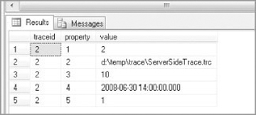
Figure 12-7 shows the output. Notice, the Property 1 row contains the @options parameter value. A trace with a Property 1 value of 1 is most likely a trace started from Profiler. The Property 2 row contains the trace filename, if any. The Property 3 row contains the maximum file size, which is 10MB in this case; and the Property 4 row contains the stop time, which has some value for this trace. The Property 5 row shows the trace’s status — in this case 1, which means that Trace is running.
The function fn_trace_geteventinfo()shows you the events and data columns that a particular trace captures, but the function returns the data with the event and data column IDs, instead of a name or explanation, so you must track down their meaning.
The function fn_trace_getfilterinfo() returns information about a particular trace’s filters like so:
 SELECT
* FROM fn_trace_geteventinfo (2)
Retrieving Data from the Trace File
You can retrieve the trace data from the file in two ways: using the function fn_trace_gettable or with SQL Server Profiler. Both are valuable in different situations.
The function fn_trace_gettable is a table-valued function, so you can read directly from the file using this function and insert the data into a table to analyze like so:
 SELECT * FROM fn_trace_gettable
( '<SQL Server Drive>:	emp	raceServerSideTrace .trc' , DEFAULT)
You can also use SELECT INTO in this query to store the result in a table. Put the trace data into a table because then you can write a T-SQL statement to query the data. For example, the TextData column is created with the ntext data type. You can alter the data type to nvarchar(max) so that you can use the string functions. You should not use the ntext or text data types anyway, because they will be deprecated in a future SQL Server release; use nvarchar(max)or varchar(max) instead. Even though the trace is running, you can still read the data from the file to which Trace is writing. You don’t need to stop the trace for that. The only gotcha in storing the trace data into a table is that the EventClass value is stored as an int value and not as a friendly name. Listing 12-2 creates a table and inserts the eventclassid and its name into that table. You can then use this table to get the event class name when you analyze the trace result stored there. You can write a query like the following to do that, assuming that you have stored the trace result in the table TraceResult:
LISTING 12-2: EventClassID_Name.sql
SELECT ECN.EventClassName, TR.
* FROM TraceResult TR
 LEFT JOIN EventClassIdToName ECN
ON ECN.EventClassID = TR.EventClass
SQL Server Profiler
SQL Server Profiler is a rich interface used to create and manage traces and analyze and replay trace results. SQL Server Profiler shows how SQL Server resolves queries internally. This enables you to see exactly what Transact-SQL statements or multidimensional expressions are submitted to the server and how the server accesses the database or cube to return result sets.
In SQL Server 2012, SQL Server profiler has been marked as being deprecated. Because of this, you should move any monitoring capabilities using this tool to the newer tools based on extended events.
You can read the trace file created using a T-SQL stored procedure with SQL Profiler. To use SQL Profiler to read the trace file, just go to the File menu and open the trace file you are interested in.
In SQL Server 2008, the server reports both the duration of an event and CPU time used by the event, in milliseconds. In SQL Server 2005, the server reports the duration of an event in microseconds (one millionth of a second) and the amount of CPU time used by the event in milliseconds (one thousandth of a second). In SQL Server 2000, the server reported both duration and CPU time in milliseconds. In SQL Server 2005, the SQL Server Profiler graphical user interface displays the Duration column in milliseconds by default, but when a trace is saved to either a file or a database table, the Duration column value is written in microseconds. If you want to display the duration column in microseconds in SQL Profiler, go to Tools ![]() Options and select the option Show Values in Duration Column in Microseconds (SQL Server 2005 Only).
Options and select the option Show Values in Duration Column in Microseconds (SQL Server 2005 Only).
Being able to capture and examine the XML plan for a particular query is very valuable when trying to troubleshoot issues with a particular query. SQL Server Profiler makes this possible using the XML Showplan option. Additionally, being able to correlate a Profiler trace with a Performance Monitor chart can help to diagnose performance problems by enabling you to correlate which queries are executing in a Profiler trace against performance counters captured in Performance Monitor. With this capability you can see exactly what was executing when a particular behavior was observed in the perfmon graph. The following sections discuss these options in more detail.
Showplan XML
You can get the query plan in an XML document and use this document later to generate the graphical query plan. Showplan output in XML format can be moved from one computer to another and thus rendered on any computer, even on computers where SQL Server is not installed. Showplan output in XML format can also be programmatically processed using XML technologies, such as XPath, XQuery, and so on. XML Showplan processing is supported in SQL Server 2005, which contains a built-in query evaluation engine for XPath and XQuery.
You can generate XML Showplan output using the following means:
- From the query editor toolbar in SQL Server Management Studio, select Display Estimated Execution Plan or Include Actual Execution Plan.
- Use the Transact-SQL Showplan SET statement options SHOWPLAN_XML and STATISTICS XML.
- Select the SQL Server Profiler event classes Showplan XML, Showplan XML for Query Compile, and Showplan XML Statistics Profile for tracing.
- Use the sys.dm_exec_query_plan dynamic management view.
XML Showplans are returned in the nvarchar (max) data type for all these methods except the last. XML Showplans are returned in the xml data type when you use this dynamic management view.
You can visit http://schemas.microsoft.com/sqlserver/2004/07/showplan/showplanxml.xsd for the XML Showplan schema, or you can look in the directory where SQL Server is installed: C:Program Files (x86)Microsoft SQL Server110ToolsBinnschemassqlserver2004�7showplan.
Chapter 13 explains how to read the query plan.
Figure 12-8 shows what a query plan looks like in SQL Profiler when you choose the Showplan XML event. This event is under the Performance object. To see these additional events, you need to click the Events Selection tab and select the Show All Events option.
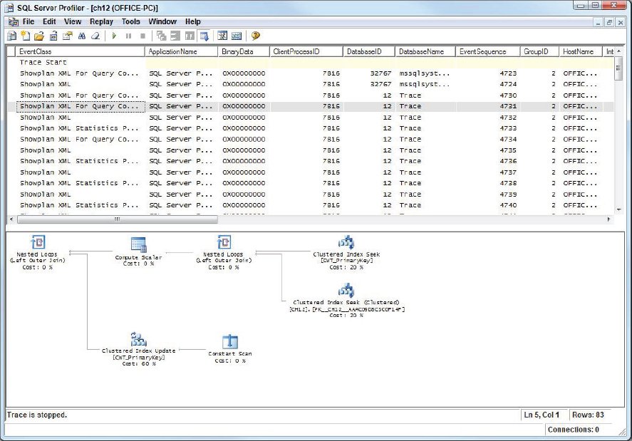
If you right-click the Showplan XML event, you see a menu item Extract Event Data. This saves the query plan with a .sqlplan extension. You can later open that file with SQL Server Management Studio or Profiler, and it displays the graphical plan exactly, as shown in Figure 12-8. You can also use File ![]() Export
Export ![]() Extract SQL Server Event in SQL Profiler to achieve the same results.
Extract SQL Server Event in SQL Profiler to achieve the same results.
When you set up the trace using Profiler, if you choose Showplan XML or Showplan Statistics Profile or Showplan XML for Query Compile, a tab shows up in the Trace Properties dialog, as shown in Figure 12-9.

Also shown in Figure 12-9 is a Deadlock XML option to store the deadlock graph in an XML document, which you can view later in SQL Management Studio or Profiler. This option is enabled only if you choose the Deadlock Graph event.
You can also use SET SHOWPLAN_XML ON before you execute the query, which can give you an estimated execution plan in XML without executing it. You can also use SET STATISTICS XML ON, which can give you an execution plan in XML format, as shown in Figure 12-10. Click the link in the XML Showplan to open an XML editor within SQL Server Management Studio.
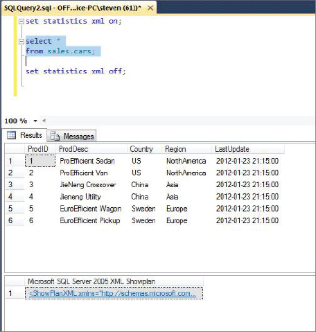
If you want to see the graphical execution plan from this XML document, you can save the document with a .sqlplan extension. Open that file in SQL Server Management Studio, and you get the graphical execution plan. Figure 12-11 shows the graphical execution plan generated from the XML document.

When the Showplan XML event class is included in a trace, the amount of overhead significantly impedes performance. Showplan XML stores a query plan that is created when the query is optimized. To minimize the overhead incurred, limit the use of this event class to traces that monitor specific problems for brief periods of time, and be sure to use the data column filter based on specifics you are going to trace.
Correlating a Trace with Windows Performance Log Data
In SQL Server 2005, a new feature was added to correlate the trace data with Performance Monitor log data based on the StartTime and EndTime data columns in the SQL trace file. If you have taken Trace and Performance Monitor data at the same time, you can relate the events that happened in SQL Server with the server activities such as processor time, disk activity, and memory usage. Figures 12-12 and 12-13 show an example of correlating trace and Performance Monitor log data.


To bring up the performance data after you open a trace file, click File ![]() Import Performance Data. That brings up the dialog shown in Figure 12-12. This option is not enabled unless you open a saved trace file. The trace file must also contain the starting and completed events for the types of activity you are interested in, including SPStarting, SPComplete, StmtStarting, StmtComplete, and so on. Without these events, the Import Performance Data option remains disabled. You can select the performance counters you are interested in and then click OK. That brings the performance counters inside the Profiler to correlate the SQL Server activity during a specific time, as shown in Figure 12-13. Move the red vertical bar to select a particular time you are interested in to see what was happening at that time in SQL Server.
Import Performance Data. That brings up the dialog shown in Figure 12-12. This option is not enabled unless you open a saved trace file. The trace file must also contain the starting and completed events for the types of activity you are interested in, including SPStarting, SPComplete, StmtStarting, StmtComplete, and so on. Without these events, the Import Performance Data option remains disabled. You can select the performance counters you are interested in and then click OK. That brings the performance counters inside the Profiler to correlate the SQL Server activity during a specific time, as shown in Figure 12-13. Move the red vertical bar to select a particular time you are interested in to see what was happening at that time in SQL Server.
If you look at the peak value for a performance counter — for example, average disk queue length — that brings up whatever query SQL Server was executing at the time. However, that doesn’t mean the query caused the disk queue length to increase exactly at that time. The query might have started a little earlier and now requests a lot of data from disk, which may cause the average disk queue length to shoot up. In short, be careful before you jump to conclusions; make sure you look at the whole picture.
Replaying a Trace
Replay is the capability to save a trace and replay it later. This functionality enables you to reproduce the activity captured in a trace. When you create or edit a trace, you can save the trace to replay it later. Be sure to choose the predefined template called TSQL_Replay when you create the trace using SQL Profiler. SQL Server needs specific events and data columns to be captured to replay the trace later. If you miss those events and data columns, SQL Server does not replay the trace. Trace replay supports debugging by using the Toggle Breakpoint and the Run to Cursor options on the SQL Server Profiler Replay menu. These options especially improve the analysis of long scripts because they can break the replay of the trace into short segments so they can be analyzed incrementally.
The following types of events are ignored when you replay the trace:
- Traces that contain transactional replication and other transaction log activity. These events are skipped. Other types of replication do not mark the transaction log, so they are not affected.
- Traces that contain operations involving globally unique identifiers (GUID). These events are skipped.
- Traces that contain operations on text, ntext, and image columns involving the bcp utility, the BULK INSERT, READTEXT, WRITETEXT, and UPDATETEXT statements, and full-text operations. These events are skipped.
- Traces that contain session binding: sp_getbindtoken and sp_bindsession system stored procedures. These events are skipped.
- SQL Server Profiler does not support replaying traces collected by Microsoft SQL Server version 7.0 or earlier.
In addition, some requirements must be met to replay the trace on the target server:
- All logins and users contained in the trace must be created already on the target and in the same database as the source.
- All logins and users in the target must have the same permissions they had in the source.
- All login passwords must be the same as those of the user who executes the replay. You can use the Transfer Login task in SSIS to transfer the logins to the target server on which you want to replay the trace.
- The database IDs on the target ideally should be the same as those on the source. However, if they are not the same, matching can be performed based on the database name if it is present in the trace, so make sure that you have the DatabaseName data column selected in the trace.
- The default database on the target server for a login should be the same as on the source when the trace was taken.
- Replaying events associated with missing or incorrect logins results in replay errors, but the replay operation continues.
Distributed Replay
New for SQL Server 2012 is Distributed Replay, a tool for replaying traces from multiple machines. While SQL profiler can replay a trace, it can only do so from a single machine. Distributed replay can also replay traces, but can do so from a pool of machines. Because of this, distributed replay provides a more scalable solution than SQL profiler, and is better at simulating mission critical workloads.
Now that there are two tools for replaying traces, the question becomes when to use which tool. As a general rule, you should use SQL profiler for all trace replays, and always for replaying traces against Analysis Services. You only need to resort to distributed replay if the concurrency in the captured trace is so high that a single server cannot sufficiently simulate the load you want to put onto the target server.
A Distributed Replay system known as a Distributed Replay Utility consists of a number of different servers, the Admin tool, the controller, a number of clients, and the target SQL Server.
Because Distributed Replay can replay a trace from multiple servers, you need to do a little additional work on the Trace file before it can be used in a distributed replay. Specifically you have to pre-process the trace file and spilt it into multiple streams of commands that are replayed from the different client servers in the distributed replay utility.
Performance Considerations When Using Trace
SQL Server tracing incurs no overhead unless it captures an event, and most events need few resources. Profiler can become expensive as you add events, and increase the amount of event data captured for each event. Normally, you see a maximum of from 10-20 percent overhead. If you see more than this, or even if this level of overhead is impacting the production system, either reduce the number of events, reduce the amount of data, or use an alternate approach. Most of the performance hit results from a longer code path; the actual resources that the trace needs to capture event data aren’t particularly CPU-intensive. In addition, to minimize the performance hit, you can define all your traces as server-side traces, avoiding the overhead of producing rowsets to send to the Profiler client.
Event Notifications
Event notifications are special database objects that send messages to the Service Broker service (see Chapter 7, “SQL Server CLR Integration,” for details on the Service Broker) with information regarding server or database events. Event notifications can be programmed against many of the same events captured by SQL Trace, but not all. Event Notifications can also be programmed against many DDL events. Unlike creating traces, event notifications can be used to perform an action inside an instance of SQL Server in response to events. Later in this chapter you see an example that shows how to create an event notification for specific events, and take actions if needed.
To subscribe to an event, you must create the Service Broker queue that receives the details regarding the event. In addition, a queue requires the Service Broker service to receive the message. Then you need to create an event notification. You can create a stored procedure and activate it when the event message is in the queue to take a certain action. This example assumes you know how the Service Broker works, so be sure to read Chapter 8, “Securing the Database Instance,” if you don’t already know about the Server Broker.
You can also be notified for grouped events. For example, if you want to be notified when a table is created, altered, or dropped, you don’t need to create three separate event notifications. You can use the group event called DDL_TABLE_EVENTS and just create one event notification to achieve the same thing. Another example is related to monitoring all the locking events using the event group TRC_LOCKS. When you create an event notification with this group, you can be notified about the following events: LOCK_DEADLOCK, LOCK_DEADLOCK_CHAIN, LOCK_ESCALATION, and DEADLOCK_GRAPH.
Refer to the BOL topic “DDL Event Groups for Use with Event Notifications” for all the event groups.
Event notifications can be used to do the following:
- Log and review changes or activity occurring on the database or server.
- Perform an action in response to an event in an asynchronous, rather than synchronous, manner.
Event notifications can offer a programming alternative to DDL triggers and SQL Trace.
Event notifications are created at the server or database level.
You can create an event notification in a database whereby you will be notified when a new table is created. To do so, perform the following steps:
1. Open the project EventNotification using SQL Server Management Studio, and then open the CreateDatabase.sql script. This script creates a database called StoreEvent for the example. Run this script.
2. Next, open the CreateQueue.sql script, shown in Listing 12-3:
LISTING 12-3: CreateQueue.sql
USE StoreEvent
 GO

 --CREATE QUEUE to receive the event details.
 IF OBJECT_ID('dbo.NotifyQueue') IS NULL
 CREATE QUEUE dbo.NotifyQueue
 WITH STATUS = ON
     ,RETENTION = OFF
 GO

 --create the service so that when event happens
 --server can send the message to this service.
 --we are using the pre-defined contract here.
 IF NOT EXISTS(SELECT * FROM sys.services WHERE name =
 'EventNotificationService')
 CREATE SERVICE EventNotificationService
 ON QUEUE NotifyQueue
 ([http://schemas.microsoft.com/SQL/Notifications/PostEventNotification])

 IF NOT EXISTS(SELECT * FROM sys.routes WHERE name = 'NotifyRoute')

 CREATE ROUTE NotifyRoute
 WITH SERVICE_NAME = 'EventNotificationService',
 ADDRESS = 'LOCAL';
GO
3. This script creates a queue in the StoreEvent database to store the event data when a table is created in the StoreEvent database. It creates a Service Broker service EventNotificationService such that SQL Server can send the message when a subscribed event happens. The route NotifyRoute helps route the message to a local SQL server instance. Run this script.
4. Now you need to create the event notification. Open the script CreateEventNotification.sql, shown in the following code snippet:
USE StoreEvent
 GO
 CREATE EVENT NOTIFICATION CreateTableNotification
 ON DATABASE
 FOR CREATE_TABLE
 TO SERVICE 'EventNotificationService', 'current database' ;
CreateEventNotification.sql
This script creates an event notification called CreateTableNotification that notifies you when a table is created in the StoreEvent database.
Messages are sent from one service to another, as discussed in Chapter 6. In this case, you have created the target end of the service, which is EventNotificationServer; the initiator end of the service is SQL Server itself.
5. When a table is created in the StoreEvent database, you get the message in the queue NotifyQueue, so create a table and run the following script to see what’s in the queue:
 SELECT CAST(message_body AS xml)
 FROM NotifyQueue
6. Following is what the final XML message in the queue looks like:
 <EVENT_INSTANCE>
   <EventType>CREATE_TABLE</EventType>
   <PostTime>2012-09-23T21:53:14.463</PostTime>
   <SPID>56</SPID>
   <ServerName>CIPHER</ServerName>
   <LoginName>REDMONDketanp</LoginName>
   <UserName>dbo</UserName>
   <DatabaseName>StoreEvent</DatabaseName>
   <SchemaName>dbo</SchemaName>
   <ObjectName>TestTable1</ObjectName>
   <ObjectType>TABLE</ObjectType>
   <TSQLCommand>
     <SetOptions ANSI_NULLS="ON" ANSI_NULL_DEFAULT="ON" ANSI_PADDING="ON"
 QUOTED_IDENTIFIER="ON" ENCRYPTED="FALSE" />
     <CommandText>CREATE TABLE TestTable1 (col1 int, col2 varchar(100), col3
 xml)
 </CommandText>
   </TSQLCommand>
 </EVENT_INSTANCE>
You can take some action with this event if you create a stored procedure and have it activated when a message arrives in the queue. You create the serverwide event in the same way. For a full list of the events for which you can be notified, you can query the sys.event_notification_event_types view. Refer to the script Metadata_EventNotification.sql to get the catalog view list that stores the metadata about event notifications.
SQL Server Extended Events
SQL Server Extended Events (XEvents) was a completely new feature for SQL Server 2008. Extended Events have been enhanced in SQL Server 2012 with increased event coverage and a new GUI interface in SSMS. Extended Events provide a deep insight into SQL Server internals and are designed to enable faster diagnosis of issues with SQL Server. They provide the capability to act either synchronously or asynchronously to SQL Events and are designed to be extremely lightweight and highly scalable. The system_health session is a lighter weight and more powerful version of the default_trace. Extended events are also lighter weight and more flexible and scalable than SQL Server Trace and SQL Profiler.
Extended events are designed to replace some of the older monitoring technologies such as SQL Server Profiler. All the events and columns available in SQL Server Profiler are available through Extended Events.
XEvent Objects
This section introduces the new objects in XEvents. The object hierarchy for XEvent objects is shown in Figure 12-14.
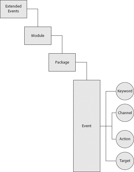
Module
The Module object is equivalent to the binary that contains the events. Module is equivalent to SQLServr.exe, or MyDll.dll if you were to write your own code and load it into SQL Server. The only place you see the module is as an attribute of the package in the DMV sys.dm_xe_packages.
Package
A package is a container object within the module. The packages that come with SQL Server can be seen in the DMV sys.dm_xe_packages. The following code lists the contents of this DMV, the results of which are shown in Table 12-1.
select name, description
from sys.dm_xe_packages
TABLE 12-1: sys.dm_xe_packages
| NAME | DESCRIPTION |
| package0 | Default package; contains all standard types, maps, compare operators, actions, and targets |
| sqlos | Extended events for SQL operating system |
| XeDkPkg | Extended events for SQLDK binary |
| sqlserver | Extended events for Microsoft SQL Server |
| SecAudit | Security Audit Events |
| Ucs | Extended events for Unified Communications Stack |
| Sqlclr | Extended events for SQL CLR |
| Filestream | Extended events for SQL Server FILESTREAM and FileTable |
| sqlserver | Extended events for Microsoft SQL Server |
As with modules, you won’t be creating any packages unless you write your own code and create your own new events.
Event
Events are the first “real” objects in the hierarchy. An event represents an occurrence of a significant activity within SQL Server. To get a better understanding of events, take a look at some of the events available. You can find these in the DMV sys.dm_xe_objects and they have a type of 'event'. The following code outputs a list of event types:
select name
from sys.dm_xe_objects
where object_type ='event'
order by name
This returns a list of 618 different events. This is quite an increase from the 254 event types that were originally available in SQL Server 2008. A select few are listed here:
checkpoint_begin
checkpoint_end
lock_acquired
lock_deadlock
lock_released
locks_lock_waits
sp_statement_completed
sp_statement_starting
sql_statement_completed
sql_statement_starting
wait_info
wait_info_external
All events have two additional attributes: Keyword and Channel. The Keyword for an event is a way to group events based on who fires the event, so keywords are memory, broker, server, and so on. The Channel for an event reflects who might be interested in the event. Following are four channels in SQL Server 2012:
- debug
- analytical
- operational
- administration
To see the Channel and Keyword for the events requires that you join several of the XEvent DMVs, as in the following code:
 select p.name as package_name
 , k.event
 , k.keyword
 , c.channel
 , k.description
 from (
 select c.object_package_guid as event_package
 , c.object_name as event
 , v.map_value as keyword
 , o.description
 from sys.dm_xe_object_columns as c inner join sys.dm_xe_map_values as v
   on c.type_name = v.name
   and c.column_value = v.map_key
   and c.type_package_guid = v.object_package_guid
 inner join sys.dm_xe_objects as o
   on o.name = c.object_name
   and o.package_guid = c.object_package_guid
 where c.name = 'keyword'
 ) as k inner join (
 select c.object_package_guid as event_package
 , c.object_name as event
 , v.map_value as channel
 , o.description
 from sys.dm_xe_object_columns as c inner join sys.dm_xe_map_values as v
   on c.type_name = v.name
   and c.column_value = v.map_key
   and c.type_package_guid = v.object_package_guid
 inner join sys.dm_xe_objects as o
   on o.name = c.object_name
   and o.package_guid = c.object_package_guid
 where c.name = 'channel'
 ) as c
 on
 k.event_package = c.event_package and k.event = c.event
 inner join sys.dm_xe_packages as p on p.guid = k.event_package
 order by keyword
 , channel
 , event
Table 12-2 shows a few of the events, including their keywords and channels.
TABLE 12-2: Select Extended Events

Action
Actions are what you want to happen when an event fires. They are invoked synchronously on the thread that fired the event. The available actions are stored in the DMV sys.dm_xe_objects with an object_type = 'action'. The action enables you to do things such as correlate a plan_handle, and T-SQL stack with a specific event. This kind of flexibility creates an incredibly powerful framework that exceeds anything that SQL Trace and SQL Profiler could do.
The following query returns all the actions available.
 select name
 from sys.dm_xe_objects
 where object_type = 'action'
 order by name
This query returns 50 actions, some of which are listed here:
attach_activity_id
attach_activity_id_xfer
callstack
collect_cpu_cycle_time
collect_system_time
create_dump_all_thread
create_dump_single_thread
database_context
database_id
debug_break
plan_handle
session_id
sos_context
sql_text
transaction_id
tsql_stack
Predicate
A predicate is a filter that is applied to the event right before the event is published. A Boolean expression, it can be either local or global and can store state.
Predicates are stored in the DMV sys.dm_xe_objects and can be seen using the following T-SQL:
 select name, description
 from sys.dm_xe_objects
 where object_type = 'pred_compare'
 order by name
 -- 77 rows

 select name, description
 from sys.dm_xe_objects
 where object_type = 'pred_source'
 order by name
 -- 44rows
Table 12-3 shows a few of the pred_compare objects.
TABLE 12-3: Selected pred_compare objects
| NAME | DESCRIPTION |
| divides_by_uint64 | Whether a uint64 divides another with no remainder |
| equal_ansi_string | Equality operator between two ANSI string values |
| greater_than_equal_float64 | Greater than or equal operator between two 64-bit double values |
| greater_than_i_sql_ansi_string | Greater than operator between two SQL ANSI string values |
| less_than_ansi_string | Less than operator between two ANSI string values |
| less_than_equal_i_unicode_string_ptr | Less than or equal operator between two UNICODE string pointer values |
| less_than_int64 | Less than operator between two 64-bit signed int values |
| not_equal_ptr | Inequality operator between two generic pointer values |
Table 12-4 lists some of the pred_source objects.
TABLE 12-4: Selected pred_source objects
| NAME | DESCRIPTION |
| Counter | Counts the number of times evaluated. |
| cpu_id | Gets the current CPU ID. |
| current_thread_id | Gets the current Windows thread ID. |
| database_id | Gets the current database ID. |
| node_affinity | Gets the current NUMA node affinity. |
| partitioned_counter | Per-CPU partitioned counter. The value is aggregated and approximate. |
| scheduler_address | Gets the current scheduler address. |
| scheduler_id | Gets the current scheduler ID. |
| session_id | Gets the current session ID. |
| system_thread_id | Gets the current system thread ID. |
| task_address | Gets the current task address. |
| task_elapsed_quantum | Gets the time elapsed since quantum started. |
| task_execution_time | Gets the current task execution time. |
| transaction_id | Gets the current transaction ID. |
| worker_address | Gets the current worker address. |
Target
A target is a way to define what you want to happen to the events you monitor. The fifteen targets defined for SQL Server 2012 are shown in the following table. Like the other XEvent objects, they can be found in the DMV sys.dm_xe_objects with an object_ type = 'target'.
The following T-SQL code returns the list of targets from sys.dm_xe_objects:
 select name, description
 from sys.dm_xe_objects
 where object_type = 'target'
 order by name
The fifteen different targets can be seen in Table 12-5.
TABLE 12-5: Targets
| NAME | DESCRIPTION |
| asynchronous_router | Route events to asynchronous listeners. |
| asynchronous_security_audit_event_log _target | Asynchronous security audit NT event log target. |
| asynchronous_security_audit_file _target | Asynchronous security audit file target. |
| asynchronous_security_audit_security _log_target | Asynchronous security audit NT security log target. |
| etw_classic_sync_target | Event Tracing for Windows (ETW) Synchronous Target. |
| Event_counter | Counts the number of occurrences of each event in the event session. |
| Event_file | Saves the event data to an XEL file, which can be archived and used for later analysis and review. You can merge multiple XEL files to view the combined data from separate event sessions. |
| Event_stream | Asynchronous live stream target. |
| histogram | Aggregates event data based on a specific event data field or action associated with the event. The histogram enables you to analyze distribution of the event data over the period of the event session. |
| pair_matching | Pairing target. |
| ring_buffer | Asynchronous ring buffer target. |
| router | Route events to listeners. |
| synchronous_security_audit_event_log _target | Synchronous security audit NT event log target. |
| synchronous_security_audit_file _target | Synchronous security audit file target. |
| synchronous_security_audit_security _log_target | Synchronous security audit NT security log target. |
Event Session
The event session is where all the objects detailed earlier are brought together to actually do something. You create the event session to define which of those objects you want to use to perform your event capture.
Event sessions are created using the DDL CREATE EVENT SESSION syntax. This one statement enables you to define all the objects you need to create a new event session. The only thing you cannot do is start the session. For transaction consistency, the session must be created first. When it has been created, it can be started using the ALTER EVENT SESSION syntax:
ALTER EVENT SESSION <session name> STATE = START
Listing 12-4 shows an example of code to create a new event session that gathers sql_text, and the tsql_stack for any SQL statement that has a duration > 30 ms. It then writes the output to the xml file specified in the target specification, and flushes results from memory to the file every second.
LISTING 12-4: XE_long_running_queries.sql
-- Create a new event session
create event session long_running_queries on server
-- Add the sql_statement_complete event
add event sqlserver.sql_statement_completed
(
     -- for this event get the sql_text, and tsql_stack
     action(sqlserver.sql_text, sqlserver.tsql_stack)
     -- Predicate on duration > 30 ms ( milli seconds )
     where sqlserver.sql_statement_completed.duration > 30
)

-- Send the output to the specified XML file
add target package0.asynchronous_file_target
(
     set filename=N'c:chapter_12_samplesXEventslong_running_queries.xel'
     , metadatafile = N'c:chapter_12_samplesXEventslong_running_queries.xem'
)
-- Specify session options,
-- max_dispatch_latency specifies how long we buffer in memory before pushing
 to the target
with (max_dispatch_latency = 1 seconds)
ALTER SESSION is probably most frequently used to start and stop sessions, but it can also be used to add or remove events from an existing session. The following code snippet shows how to start the session you created in Listing 12-4.
-- Which event session do we want to alter
alter event session long_running_queries on server
-- Now make any changes
-- change the state to start
state = start
The code shown in Listing 12-5 below shows how to use ALTER SESSION to add an additional event to the existing event session.
LISTING 12-5: XE_alter_long_running_queries.sql
-- Which event session do we want to alter
alter event session long_running_queries on server
-- Now make any changes
-- add another event, this time the long_io_detected event
add event sqlserver.long_io_detected
(
-- for this event get the sql_text, and tsql_stack
     action(sqlserver.sql_text, sqlserver.tsql_stack)
     -- No predicate, we want all of these to see if there is any correlation
)
To see which sessions are currently active, use the following queries:
 select
* from sys.dm_xe_sessions

 select
* from sys.dm_xe_session_events
Catalog Views
Following are several of the catalog views that expose information about XEvents:
- server_event_sessions
- server_event_session_targets
- server_event_session_fields
- server_event_session_events
- server_event_session_actions
DMVs
You have already seen some of the Extended Event DMVs in action. For completeness, here is the full list:
- sys.dm_xe_map_values: Returns a mapping of internal numeric keys to human-readable text.
- sys.dm_xe_object_columns: Returns the schema information for all the objects.
- sys.dm_xe_objects: Returns a row for each object exposed by an event package. Objects can be one of the following:
- Events: Indicate points of interest in an execution path. All events contain information about a point of interest.
- Actions: Run synchronously when events fire. An action can append run-time data to an event.
- Targets: Consume events, either synchronously on the thread that fires the event or asynchronously on a system-provided thread.
- Predicate sources: Retrieve values from event sources for use in comparison operations. Predicate comparisons compare specific data types and return a Boolean value.
- Types: Encapsulate the length and characteristics of the byte collection, which is required to interpret the data.
- sys.dm_xe_packages: Lists all the packages registered with the extended events engine.
- sys.dm_xe_session_event_actions: Returns information about event session actions. Actions are executed when events are fired. This management view aggregates statistics about the number of times an action has run and the total run time of the action.
- sys.dm_xe_session_events: Returns information about session events. Events are discrete execution points. Predicates can be applied to events to stop them from firing if the event does not contain the required information.
- sys.dm_xe_session_object_columns: Shows the configuration values for objects that are bound to a session.
- sys.dm_xe_session_targets: Returns information about session targets.
- sys.dm_xe_sessions: Returns information about an active extended events session. This session is a collection of events, actions, and targets.
Working with Extended Event Sessions
There are several ways that you can create, modify, display, and analyze sessions and session data.
You can manipulate extended events using DDL in T-SQL as you saw in some of the previous examples. There are additional T-SQL examples on creating Extended Event Sessions later in this section.
There are two graphical user interfaces that you can use with Extended Events: The New Session Wizard and the New Session UI.
New Session Wizard
The new session wizard guides you through the creation of a new session with the following steps:
1. Launch it from SQL Server Management Studio. Open the Management node, then the Extended Events Node, and then the Session Node. Right click on Sessions, and choose New Session Wizard. This launches the New Session Wizard and displays the Introduction page as shown in Figure 12-15.

2. Select Next to move onto the set session properties page. Here you provide a session name, and select if you want the session to start up each time the server starts (see Figure 12-16). For this example, enter the name chapter_12_test.

3. Select Next to move onto the Choose template page. Here you choose a predefined template for the events in the template, or you can select to not use a template, and manually select events. In this example, select “Use this event session template” which populates the list of event session templates shown in Figure 12-17. For this example select the “Query Wait Statistics” template and select Next.

4. The Next page in the Wizard is the Select Events To Capture page (see Figure 12-18). Because you chose to use a template, this is already populated with the events from the template. You can see the event selected in the template in the selected events box. Because you used a template, you don’t need to do anything here.
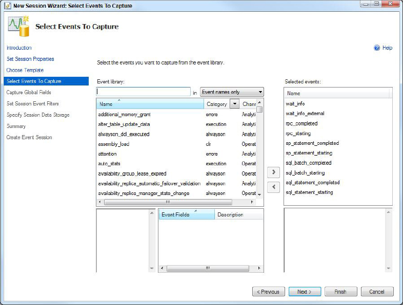
5. Select Next to move onto the Capture Global Fields page. This page is shown in Figure 12-19. Again, because you selected a template, a number of global fields are already preselected. The preselected fields are those with a checkbox next to them. In Figure 12-19 you can see client_app_name, and database_id are checked. Scrolling down shows the other fields that are selected from the template.

6. Select Next to move onto the Set Session Event Filters page (see Figure 12-20). Here you can select any filters (also known as predicates) that would restrict the amount of data to be captured. For this example you are not going to apply any filters.

7. Select Next to move onto the Specify Session Data Storage page (see Figure 12-21). Here you can specify where you want the data to be collected. The two options are to save data to a file for alter analysis, or to put it into a ring buffer. For this example, select Save data to a file for later analysis (event_file target), and leave the default values for filename, max file size, enable file rollover, and max number of file.

8. Select Next to move onto the Summary page. This page shown in Figure 12-22 provides a summary of the selections made throughout the wizard. This provides one last opportunity to confirm the values selected before the wizard applies these settings and creates the new event session.
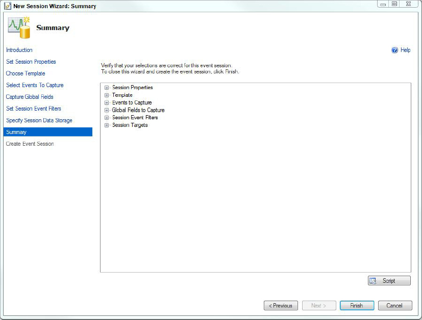
9. Select Finish and the wizard creates the new event session. If it creates the event session successfully, you see the success page and have the option to start the event session immediately and watch live data as it is captured. The Create Event Session success screen is shown in Figure 12-23. Select both options: start the event session immediately, and watch live data on screen as shown in Figure 12-23.

10. Select Close to close the wizard, start the event session, and watch live data being captured. The wizard closes, and SSMS displays a new tab showing the Live Data for the new session.
New Session UI
The New Session UI is launched from SQL Server Management Studio. To start using this interface, perform the following steps:
1. Open the Management node, then the Extended Events Node, and then the Session Node. Right click on Sessions, and choose New Session. This opens the New Session UI on the General Page. Enter a session name of chapter_12_test2, and select the Connection Tracking template. Select to start the event session at server startup. You see a page similar to that shown in Figure 12-24.

2. Select the Events Page to see which events have been pre selected with this template (see Figure 12-25). Because you selected a template, there is no need to change anything here.

3. Select the Data Storage page to define how the data is going to be stored. The default here is to store data into a ring_buffer target. To change this, select Add which adds a new line to the list of targets, with a drop down for “Please choose a target type.” Expand this drop down and you see the full set of targets, as shown in Figure 12-26.
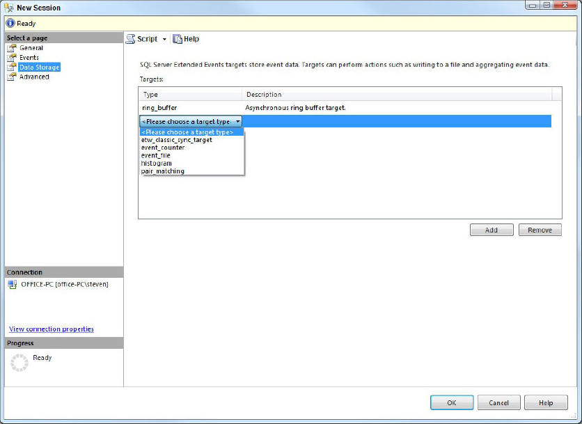
4. Select event_file. This adds a set of target specific properties below the list of targets. For this example, the default values are acceptable, so there is no need to change them.
5. Select the Advanced page to specify advanced settings for the New Session. The Advanced page is shown in Figure 12-27. These settings are acceptable for this example.
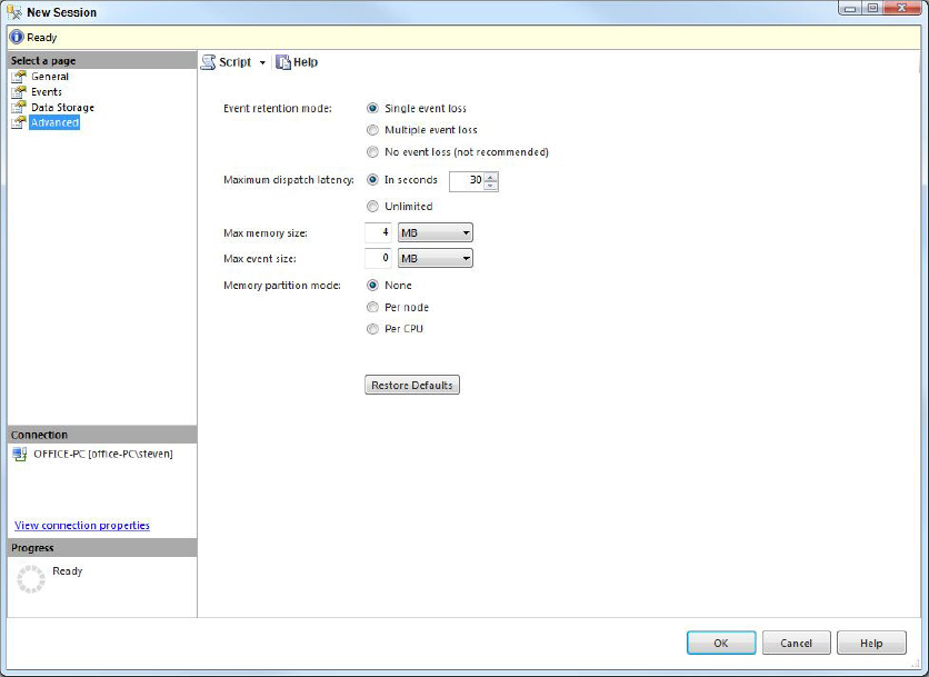
6. At this point you have examined all the options for creating the new session. To create the new session, select OK. The UI disappears, and if you go look in SSMS under Management ![]() Extended Events
Extended Events ![]() Sessions, you see that a new session called chapter_12_test2 has been created. Because of the options you selected, it is not currently running.
Sessions, you see that a new session called chapter_12_test2 has been created. Because of the options you selected, it is not currently running.
7. To start the new session, right click it, and select Start Session. To view live data for the session, right click it and select Watch Live Data.
Editing a Session
To edit a session, select it in SSMS right click its node, and select Properties. This brings up the same set of pages seen in the New Session UI, but this time preloaded with the session info, and with some options disabled. Select properties on the chapter_12_test2 session to display the dialog seen in Figure 12-28.

Using this dialog, you can edit many of the session properties. There are additional options throughout the session UI that have not been discussed here. Most of these options are self explanatory, but it is recommended to explore these in conjunction with the available documentation in Books Online.
MONITORING WITH DYNAMIC MANAGEMENT VIEWS AND FUNCTIONS
Dynamic management views (DMVs) and dynamic management functions (DMFs) are a godsend to the DBA. They provide plenty of information about server and database state. DMVs, and DMF’s are designed to give you a window into what’s going on inside SQL Server. They return server state information that you can use to monitor the health of a server instance, diagnose problems, and tune performance. Following are two types of DMVs and DMFs:
- Server-scoped dynamic management views and functions
- Database-scoped dynamic management views and functions
All DMVs and functions exist in the sys schema and follow the naming convention dm_* respectively. To view the information from a server-scoped DMV, you have to grant the SERVER VIEW STATE permission to the user. For database-scoped DMVs and functions, you have to grant the VIEW DATABASE STATE permission to the user. After you grant the VIEW STATE permission, that user can see all the views; to restrict the user, deny the SELECT permission on the dynamic management views or functions that you do not want the user to access. The following example grants the VIEW SERVER STATE permission to the user Aish:
GRANT VIEW SERVER STATE TO [MyDomAish]
If you want the user [MyDomAish] to be restricted from viewing information in the view sys.dm_os_wait_stats, you need to DENY SELECT as follows:
DENY SELECT ON sys.dm_os_wait_stats TO [MyDomAish]
DMVs and DMFs are generally divided into the following categories:
- Always On Availability Group
- Change Data Capture–related
- Change Tracking–related
- CLR-related
- Database mirroring–related
- Database-related
- Execution-related
- Filestream and FileTable
- Full-Text-Search and Semantic Search
- Index-related
- I/O-related
- Object related
- Query notifications related
- Replication–related
- Resource Governor
- Security–related
- Service Broker–related
- SQL Server OS–related
- Transaction-related
Rather than describe all the views here, this section looks at examples for the common tasks a DBA would perform to monitor a SQL Server. For details about all the DMVs and functions, please refer to the Books Online topic “Dynamic Management Views and Functions.”
Following are some of the scenarios in which you can use DMVs and functions. You can also open a sample DMV to get all the scripts. Following are just a few examples, but in the sample DMV solution you can find many examples for monitoring your SQL Server.
What’s Going on Inside SQL Server?
The following sections illustrate querying the DMVs to determine what is currently going on inside SQL Server.
Currently Running Queries
Listing 12-6 shows the SQL text for currently running queries. It helps you find which queries are currently running and displays the SQL text for each currently running query. This is useful when you try to determine what is currently running in terms of T-SQL code, and not just SPIDs / session_ids.
LISTING 12-6: Current running queries.sql
select r.session_id
   ,r.status
   ,substring(qt.text,r.statement_start_offset/2,
   (case when r.statement_end_offset = -1
   then len(convert(nvarchar(max), qt.text)) * 2
   else r.statement_end_offset end - r.statement_start_offset)/2)
   as query_text
   ,qt.dbid
   ,qt.objectid
   ,r.cpu_time
   ,r.total_elapsed_time
   ,r.reads
   ,r.writes
   ,r.logical_reads
   ,r.scheduler_id
 from sys.dm_exec_requests as r
 cross apply sys.dm_exec_sql_text(sql_handle) as qt
 inner join sys.dm_exec_sessions as es on r.session_id = es.session_id
 where es.is_user_process = 1
 order by r.cpu_time desc
Who Is Using Which Resources?
Listing 12-7 samples the system tables which are now deprecated. It samples sysprocesses over a 10-second interval and reports on the delta between the first and second sample. While sysprocesses is deprecated, it has all the information nicely formatted in one place, whereas the corresponding DMVs require joins to multiple DMVs. Because sysprocesses is so easy to use, you are better off continuing to use sysprocesses for as long as it is available:
LISTING 12-7: Resource Usage.sql
 -- Who is using all the resources?
 select spid, kpid, cpu, physical_io, memusage, sql_handle, 1 as sample,
 getdate() as sampleTime, hostname, program_name, nt_username
 into #Resources
 from master..sysprocesses

 waitfor delay '00:00:10'

 Insert #Resources
 select spid, kpid, cpu, physical_io, memusage, sql_handle, 2 as sample,
 getdate() as sampleTime, hostname, program_name, nt_username
 from master..sysprocesses

 -- Find the deltas
 select r1.spid
 , r1.kpid
 , r2.cpu - r1.cpu as d_cpu_total
 , r2.physical_io - r1.physical_io as d_physical_io_total
 , r2.memusage - r1.memusage as d_memusage_total
 , r1.hostname, r1.program_name, r1.nt_username
 , r1.sql_handle
 , r2.sql_handle
 from #resources as r1 inner join #resources as r2 on r1.spid = r2.spid
     and r1.kpid = r2.kpid
 where r1.sample = 1
 and r2.sample = 2
 and (r2.cpu - r1.cpu) > 0
 order by (r2.cpu - r1.cpu) desc

 select r1.spid
 , r1.kpid
 , r2.cpu - r1.cpu as d_cpu_total
 , r2.physical_io - r1.physical_io as d_physical_io_total
 , r2.memusage - r1.memusage as d_memusage_total
 , r1.hostname, r1.program_name, r1.nt_username
 into #Usage
 from #resources as r1 inner join #resources as r2 on r1.spid = r2.spid
      and r1.kpid = r2.kpid
 where r1.sample = 1
 and r2.sample = 2
 and (r2.cpu - r1.cpu) > 0
 order by (r2.cpu - r1.cpu) desc

 select spid, hostname, program_name, nt_username
 , sum(d_cpu_total) as sum_cpu
 , sum(d_physical_io_total) as sum_io
 from #Usage
 group by spid, hostname, program_name, nt_username
 order by 6 desc

 drop table #resources
drop table #Usage
Who Is Waiting?
Listing 12-8, which shows the tasks that are currently waiting, uses the same sampling principle as the preceding query:
LISTING 12-8: Who is waiting.sql
select
* , 1 as sample
 , getdate() as sample_time
 into #waiting_tasks
 from sys.dm_os_waiting_tasks

 waitfor delay '00:00:10'

 insert #waiting_tasks
 select
* , 2
 , getdate()
 from sys.dm_os_waiting_tasks

 -- figure out the deltas
 select w1.session_id
 , w1.exec_context_id
 ,w2.wait_duration_ms - w1.wait_duration_ms as d_wait_duration
 , w1.wait_type
 , w2.wait_type
 , datediff(ms, w1.sample_time, w2.sample_time) as interval_ms
 from #waiting_tasks as w1 inner join #waiting_tasks as w2 on w1.session_id =
 w2.session_id
 and w1.exec_context_id = w2.exec_context_id
 where w1.sample = 1
 and w2.sample = 2
 order by 3 desc

 -- select * from #waiting_tasks
drop table #waiting_tasks
Wait Stats
Listing 12-9 samples the wait stats to see what has changed over the sample period:
LISTING 12-9: Wait Stats.sql
select *, 1 as sample, getdate() as sample_time
 into #wait_stats
 from sys.dm_os_wait_stats

 waitfor delay '00:00:30'
 insert #wait_stats
 select *, 2, getdate()
 from sys.dm_os_wait_stats

 -- figure out the deltas

 select w2.wait_type
 ,w2.waiting_tasks_count - w1.waiting_tasks_count as d_wtc
 , w2.wait_time_ms - w1.wait_time_ms as d_wtm
 , cast((w2.wait_time_ms - w1.wait_time_ms) as float) /
 cast((w2.waiting_tasks_count - w1.waiting_tasks_count) as float) as avg_wtm
 , datediff(ms, w1.sample_time, w2.sample_time) as interval
 from #wait_stats as w1 inner join #wait_stats as w2 on w1.wait_type =
 w2.wait_type
 where w1.sample = 1
 and w2.sample = 2
 and w2.wait_time_ms - w1.wait_time_ms > 0
 and w2.waiting_tasks_count - w1.waiting_tasks_count > 0
 order by 3 desc
drop table #wait_stats
Viewing the Locking Information
Listing 12-10 can help you get the locking information in a particular database:
LISTING 12-10: Locks.sql
SELECT l.resource_type, l.resource_associated_entity_id
 ,OBJECT_NAME(sp.OBJECT_ID) AS ObjectName
 ,l.request_status, l.request_mode,request_session_id
 ,l.resource_description
 FROM sys.dm_tran_locks l
 LEFT JOIN sys.partitions sp
  ON sp.hobt_id = l.resource_associated_entity_id
WHERE l.resource_database_id = DB_ID()
Viewing Blocking Information
Listing 12-11 returns blocking information on your server:
LISTING 12-11: Blocking.sql
SELECT
 t1.resource_type
 ,t1.resource_database_id
 ,t1.resource_associated_entity_id
 ,OBJECT_NAME(sp.OBJECT_ID) AS ObjectName
 ,t1.request_mode
 ,t1.request_session_id
 ,t2.blocking_session_id
 FROM sys.dm_tran_locks as t1
 JOIN sys.dm_os_waiting_tasks as t2
   ON t1.lock_owner_address = t2.resource_address
 LEFT JOIN sys.partitions sp
ON sp.hobt_id = t1.resource_associated_entity_id
Index Usage in a Database
Listing 12-12 can give you index usage for the database in which you run the query. It creates a table and stores the results in that table so that you can analyze it later. This query can be helpful to determine which indexes are truly useful in your application. Make sure you run these queries for several days because this can give you a better idea of the overall picture than looking at data for just one day. Keep in mind that dynamic management views are volatile, and whenever SQL Server is restarted, these views are initialized again.
LISTING 12-12: Index Usage Stats.sql
-------------------------------------------------------------------------
 IF OBJECT_ID('dbo.IndexUsageStats') IS NULL
 CREATE TABLE dbo.IndexUsageStats
 (
  IndexName sysname NULL
 ,ObjectName sysname NOT NULL
 ,user_seeks bigint NOT NULL
 ,user_scans bigint NOT NULL
 ,user_lookups bigint NOT NULL
 ,user_updates bigint NOT NULL
 ,last_user_seek datetime NULL
 ,last_user_scan datetime NULL
 ,last_user_lookup datetime NULL
 ,last_user_update datetime NULL
 ,StatusDate datetime NOT NULL
 ,DatabaseName sysname NOT NULL
 )

 GO
 ----Below query will give you index USED per table in a database.
 INSERT INTO dbo.IndexUsageStats
 (
  IndexName
 ,ObjectName
 ,user_seeks
 ,user_scans
 ,user_lookups
 ,user_updates
 ,last_user_seek
 ,last_user_scan
 ,last_user_lookup
 ,last_user_update
 ,StatusDate
 ,DatabaseName
 )
 SELECT
  si.name AS IndexName
 ,so.name AS ObjectName
 ,diu.user_seeks
 ,diu.user_scans
 ,diu.user_lookups
 ,diu.user_updates
 ,diu.last_user_seek
 ,diu.last_user_scan
 ,diu.last_user_lookup
 ,diu.last_user_update
 ,GETDATE() AS StatusDate
 ,sd.name AS DatabaseName
 FROM sys.dm_db_index_usage_stats  diu
 JOIN sys.indexes si
   ON diu.object_id = si.object_id
  AND diu.index_id = si.index_id
 JOIN sys.all_objects so
   ON so.object_id = si.object_id
 JOIN sys.databases sd
   ON sd.database_id = diu.database_id
 WHERE is_ms_shipped <> 1
AND diu.database_id = DB_ID()
Indexes Not Used in a Database
Listing 12-13 can give you information about which indexes are not being used. If certain indexes are not used, then you should consider dropping them because they take unnecessary time to create or maintain. The results stored in the table, NotUsedIndexes, indicate which indexes are not used. Make sure you run this query for several days because this can give you a better idea of the overall picture than looking at data for just one day. Keep in mind that dynamic management views are volatile, and whenever SQL Server is restarted, these views are initialized again.
LISTING 12-13: Indexes not being used.sql
--------------------------------------------------------------------------
 --This will store the indexes which are not used.
 IF OBJECT_ID('dbo.NotUsedIndexes') IS NULL
 CREATE TABLE dbo.NotUsedIndexes
 (
  IndexName sysname NULL
 ,ObjectName sysname NOT NULL
 ,StatusDate datetime NOT NULL
 ,DatabaseName sysname NOT NULL
 )

 ----Below query will give you indexes which are NOT used per table in a database.
 INSERT dbo.NotUsedIndexes
 (
  IndexName
 ,ObjectName
 ,StatusDate
 ,DatabaseName
 )
 SELECT
  si.name AS IndexName
 ,so.name AS ObjectName
 ,GETDATE() AS  StatusDate
 ,DB_NAME()
 FROM sys.indexes si
 JOIN sys.all_objects so
   ON so.object_id = si.object_id
 WHERE si.index_id NOT IN (SELECT index_id
                           FROM sys.dm_db_index_usage_stats diu
                           WHERE si.object_id = diu.object_id
                             AND si.index_id = diu.index_id
                           )
AND so.is_ms_shipped <> 1
View Queries Waiting for Memory Grants
Listing 12-14 indicates the queries waiting for memory grants. SQL Server analyzes a query and determines how much memory it needs based on the estimated plan. If memory is not available at that time, the query is suspended until the memory required is available. If a query is waiting for a memory grant, an entry shows up in the DMV sys.dm_exec_query_memory_grants:
LISTING 12-14: waiting for memory grants.sql
SELECT
  es.session_id AS SPID
 ,es.login_name
 ,es.host_name
 ,es.program_name, es.status AS Session_Status
 ,mg.requested_memory_kb
 ,DATEDIFF(mi, mg.request_time
 , GETDATE()) AS [WaitingSince-InMins]
 FROM sys.dm_exec_query_memory_grants mg
 JOIN sys.dm_exec_sessions es
   ON es.session_id = mg.session_id
 WHERE mg.grant_time IS NULL
 ORDER BY mg.request_time
Connected User Information
Listing 12-15 can tell you which users are connected, and how many sessions each of them has open:
LISTING 12-15: Connected Users.sql
SELECT login_name
 , count(session_id) as session_count
 FROM sys.dm_exec_sessions
 GROUP BY login_name
Filegroup Free Space
Listing 12-16 indicates how much free space remains in each filegroup. This is valuable when your database uses multiple filegroups. Please note that this query uses catalog views rather than DMVs.
LISTING 12-16: filegroup free space.sql
-- Find the total size of each Filegroup
 select data_space_id, (sum(size)*8)/1000 as total_size_MB
 into #filegroups
 from sys.database_files
 group by data_space_id
 order by data_space_id

 -- Find how much we have allocated in each FG
 select ds.name, au.data_space_id
 , (sum(au.total_pages) * 8)/1000 as Allocated_MB
 , (sum(au.used_pages) * 8)/1000 as used_MB
 , (sum(au.data_pages) * 8)/1000 as Data_MB
 , ((sum(au.total_pages) -  sum(au.used_pages) ) * 8 )/1000 as Free_MB
 into #Allocations
 from sys.allocation_units as au inner join sys.data_spaces as ds
     on au.data_space_id = ds.data_space_id
 group by ds.name, au.data_space_id
 order by au.data_space_id
 -- Bring it all together
 select f.data_space_id
 , a.name
 , f.total_size_MB
 , a.allocated_MB
 , f.total_size_MB - a.allocated_MB as free_in_fg_MB
 , a.used_MB
 , a.data_MB
 , a.Free_MB
 from #filegroups as f inner join #allocations as a
 on f.data_space_id = a.data_space_id
 order by f.data_space_id

 drop table #allocations

 drop table #filegroups
Query Plan and Query Text for Currently Running Queries
Use the following query to find out the query plan in XML and the query text for the currently running batch for a particular session. Make sure that you use a grid to output the result in SQL Server Management Studio. When you get the result, you can click the link for the XML plan, which opens an XML editor inside Management Studio. If you want to look at the graphical query plan from this XML plan, click on the link to the XML plan, and it opens in anew window in SSMS. Listing 12-17 provides the query:
LISTING 12-17: query plan for running queries.sql
SELECT
  er.session_id
 ,es.login_name
 ,er.request_id
 ,er.start_time
 ,QueryPlan_XML = (SELECT query_plan FROM
 sys.dm_exec_query_plan(er.plan_handle))
 ,SQLText = (SELECT Text FROM sys.dm_exec_sql_text(er.sql_handle))
 FROM sys.dm_exec_requests er
 JOIN sys.dm_exec_sessions es
   ON er.session_id = es.session_id
 WHERE es.is_user_process = 1
ORDER BY er.start_time ASC
Memory Usage
Listing 12-18 indicates the memory used, in KB, by each internal SQL Server component:
LISTING 12-18: memory usage.sql
SELECT
  name
 ,type
 ,SUM(single_pages_kb + multi_pages_kb) AS MemoryUsedInKB
 FROM sys.dm_os_memory_clerks
 GROUP BY name, type
 ORDER BY SUM(single_pages_kb + multi_pages_kb) DESC
Buffer Pool Memory Usage
Listing 12-19 lists out all the objects within the buffer pool, along with the amount of space used by each. This is a great way to see who uses the Buffer Pool:
LISTING 12-19: Buffer Pool Memory Usage.sql
SELECT count(*)AS cached_pages_count
    ,name ,index_id
FROM sys.dm_os_buffer_descriptors AS bd
    INNER JOIN
    (
        SELECT object_name(object_id) AS name
            ,index_id ,allocation_unit_id
        FROM sys.allocation_units AS au
            INNER JOIN sys.partitions AS p
                ON au.container_id = p.hobt_id
                    AND (au.type = 1 OR au.type = 3)
        UNION ALL
        SELECT object_name(object_id) AS name
            ,index_id, allocation_unit_id
        FROM sys.allocation_units AS au
            INNER JOIN sys.partitions AS p
                ON au.container_id = p.partition_id
                    AND au.type = 2
    ) AS obj
        ON bd.allocation_unit_id = obj.allocation_unit_id
WHERE database_id = db_id()
GROUP BY name, index_id
ORDER BY cached_pages_count DESC;
Another aspect of monitoring that is frequently overlooked is monitoring the various log files available. SQL Server writes its own error log, and then there are the Windows Event logs, and you may find events logged in the Application, Security, or System Event logs.
Traditionally, the SQL Server and Windows Event logs have been viewed through separate applications: Windows Logs through the Windows Event Viewer, and SQL Logs through a text editor. The SQL Server Management Studio Log File viewer enables you to combine both sets of logs into a combined view. There are root level nodes for SQL Server, SQL Server Agent, Database Mail, and Windows NT that enable you to do this.
Monitoring the SQL Server Error Log
The SQL Server Error log is the location where SQL Server writes all its error information, and also a lot of additional informational messages about how it is working and what it is doing.
The error log is a text file written to the C:Program FilesMicrosoft SQL ServerMSSQL11.MSSQLSERVERMSSQLLog folder. A new log file is opened each time the SQL Server process starts. SQL Server keeps seven log files: the current one is called simply errorlog, and the oldest one is called errorlog.6.
The error log contains a lot of useful information. It is definitely the place to go looking for deadlock information after the relevant deadlock trace flags have been enabled.
Anytime a significant issue occurs, the first place to search for additional information should be the SQL Server Error Log. Additionally, both Event Notifications and Extended Events can be used if additional data is required to help troubleshoot a particular issue.
Monitoring the Windows Event Logs
Three Windows event logs may hold entries of relevance to a SQL Server event:
- Application event log
- Security event log
- System event log
These event logs contain additional event information about the server environment, other processes/applications operating on the server, and also additional information about the SQL Server process that may not be logged into the SQL Server Error log. These logs should be another place that you go to look for additional information about any issues that arise with SQL Server.
New to SQL Server 2008 was the Management Data Warehouse (MDW) and Data Collection. This was a new framework for data collection, storage, and reporting.
SQL Server 2008 R2 added the SQL Utility, the Utility Control Point (UCP), and the Utility Management Data Warehouse (UMDW) as a new location for data storage. The SQL Utility is a container for “managed instances” of SQL Server. The UMDW is a destination for data collection. The UCP data collector sets differ from the MDW in the granularity of data being collected. The MDW data collector is focused on troubleshooting individual queries. The UCP data collector set focuses on higher level system resource usage and is there to help the DBA determine when a SQL instance is under- or over-utilized. The UCP also provides additional reporting capabilities that were not available in SQL Server 2008 RTM.
For SQL Server 2012, you get the basics of Data Collection, a few Data Collection sets, the Management Data Warehouse, and some reports.
Following is a list of the basic concepts:
- Data provider: A data provider is a source of data to be captured. SQL Server 2012 has four data providers:
- SQL Trace
- Performance Monitor Counters
- T-SQL
- Query Activity
- Collection item: A collection item is a specific item of data to be collected. This might be a single performance monitor counter, a SQL Trace event, or a T-SQL query of a DMV.
- Collection set: A collection set is a logical grouping of collection items that are collected together. This might be all the performance counters monitoring disk I/O, or all the SQL trace events to look for long-running queries.
- Management Data Warehouse (MDW): The Management Data Warehouse is where the items in each collection set are stored. It is the repository of historical data that you have collected. This can be either an MDW, or a UMDW. MDW data collections can be written to a UMDW, but UMDW data collections cannot be written to an MDW.
- Target servers: The target servers are the systems that you want to monitor. Ideally, the MDW should be on a separate server. If it’s on one of the target servers, you run the risk of recording activity about the data collection, rather than the target server you are actually interested in.
- Data collection process: Data collection is performed by a series of SQL Agent jobs running SSIS packages that perform the data collection. Data is then captured based on the schedule defined for each collection set. It is then cached and written only to the MDW when the current buffer is full. This helps optimize I/O to the MDW.
You should expect to consume between 200–400MB/day for each server being monitored. These figures come from using the basic set of data collection sets, with 200MB per day for an idle server, and 400MB per day for a busy server.
System Data Collection Sets
Three system data collection sets ship with SQL Server 2012:
- Disk Usage: The Disk Usage system collector set collects disk usage performance counters. It is helpful for monitoring disk usage. The collected data is cached and then uploaded to the warehouse every 6 hours, where it is retained for 90 days.
- Query Activity: The Query Activity system collection set captures query activity on the target server. It collects data from the server every 15 minutes and helps you identify the most interesting queries running on a server without having to run a Profiler trace. It captures the top three queries from several different resource usage categories.
- Server Activity: The Server Activity system collection set collects a set of performance counters. Wait Statistics, Scheduler, Performance Counters, and Memory Counters are collected every 60 seconds. The active sessions and requests are collected every 10 seconds. The data is uploaded to the warehouse every 5 minutes and is deleted from the warehouse after 14 days.
Viewing Data Collected by the System Data Collection Sets
Along with the system data collection sets is a set of reports that displays the history collected in the Management Data Warehouse for each of these data collection sets. To access these reports in SQL Server Management Studio, follow these steps:
1. Open Object Explorer and select Management ![]() Data Collection
Data Collection ![]() System Data Collection Sets. Under the System Data Collection Sets node, you see the three system data collection sets listed.
System Data Collection Sets. Under the System Data Collection Sets node, you see the three system data collection sets listed.
2. To see the reports, right-click on a data collection set node (for example, Disk Usage) and select the reports item from the menu.
3. Then select Reports ![]() Historical
Historical ![]() Disk Usage Summary. Figure 12-29 shows this navigation path. The Disk Usage report displays, showing the history of disk usage data stored in the Management Data Warehouse. It look something like the report shown in Figure 12-30.
Disk Usage Summary. Figure 12-29 shows this navigation path. The Disk Usage report displays, showing the history of disk usage data stored in the Management Data Warehouse. It look something like the report shown in Figure 12-30.


4. Click a database name to see the detailed report for that database, as shown in Figure 12-31.

Creating Your Own Data Collection Set
After seeing the system data collection sets, the next step is to set up your own custom data collection sets. Currently, there is no wizard or easy user interface to handle this process, so you need to write T-SQL to execute the steps required. Fortunately, there are only a couple of simple steps. The hardest part is determining what data you want to collect, where it needs to come from, and what schedule you want to capture the data on.
For this example you create a custom collection set to execute a T-SQL query that queries the max ID from an example table that has a high insertion rate. This information enables you to report on insertion rates over a period of time.
You first need to create the sample table, which can live in either an existing database or a new database that you create. In this example, the T-SQL to create a 50MB database in the default location is included with the table-creation code. The steps needed to complete this are described along with the code.
1. Create the sample database and table:
 CREATE DATABASE [ch12_samples] ON  PRIMARY
 ( NAME = N'ch12_samples'
 , FILENAME = N'C:Program FilesMicrosoft SQL
  ServerMSSQL11.MSSQLSERVERMSSQLDATAch12_samples.mdf'
 , SIZE = 51200KB
 , MAXSIZE = UNLIMITED
 , FILEGROWTH = 1024KB )
  LOG ON
 ( NAME = N'ch12_samples_log'
 , FILENAME = N'C:Program FilesMicrosoft SQL
 ServerMSSQL11.MSSQLSERVERMSSQLDATAch12_samples_log.ldf'
 , SIZE = 10240KB
 , MAXSIZE = 2048GB
 , FILEGROWTH = 10%)
 GO

 create table Sales (
 ID int identity (1,1) not null,
 sku int not null,
 quantity int not null
 )
 go

 -- insert some sales
 insert sales (sku, quantity) values (1,1)
2. Create the collection set to get the max (id)every hour, and keep this for 45 days in the Management Data Warehouse:
-- Create the collection set
 -- Make sure this runs in msdb as that's where the DC SPs live.
 use msdb
 GO

 -- Find the uid for the schedule you want to use which is every 60 minutes
 declare @schedule_uid uniqueidentifier
 select @schedule_uid = (select schedule_uid
   from sysschedules_localserver_view
     where name=N'CollectorSchedule_Every_60min')

 -- Create a new custom collection set
 declare @collection_set_id int
 exec dbo.sp_syscollector_create_collection_set
     @name = N'Sample insertion rate',
     @schedule_uid = @schedule_uid,  -- 60 minutes
     @collection_mode = 1, -- Set collection mode to non cached,
 ie collection and upload are on the same schedule
     @days_until_expiration = 45, -- Keep data for 45 days
     @description = N'Sample max(id) so we can
 determine hourly insertion rates',
     @collection_set_id = @collection_set_id output

 select @collection_set_id as collection_set_id

 declare @paramters xml
 declare @collection_item_id int
 declare @collection_type_uid uniqueidentifier

 -- Create the XML parameters for the collection item
 select @paramters = convert(xml,
     N'<TSQLQueryCollector>
         <Query>
           <Value>select max(id) as max_id from sales</Value>
           <OutputTable>max_sales_id</OutputTable>
         </Query>
         <Databases>
             <Database>Ch13_samples</Database>
         </Databases>
       </TSQLQueryCollector>')

 -- Find the Collector type you want to use which is TSQL
 select @collection_type_uid  = collector_type_uid
 from syscollector_collector_types
 where name = 'Generic T-SQL Query Collector Type'

 -- Create the new collection item
 exec dbo.sp_syscollector_create_collection_item
     @collection_set_id = @collection_set_id,
     @collector_type_uid = @Collection_type_uid,
     @name = 'Sales max ID',
     @frequency = 60,
     @parameters = @paramters,
     @collection_item_id = @collection_item_id output;

 -- report the ID that just got created
 select @collection_item_id as collection_item_id

 -- start the collection set
 exec dbo.sp_syscollector_start_collection_set
     @Collection_set_id = @collection_set_id
Now you have created a new custom snapshot that contains the max ID from the sales table, sampled over time. This enables you to report on the growth of records in the sales table.
Examining the Data You Collected
The data collected is stored in the Management Data Warehouse. From the preceding example, there is now a new custom snapshot table created, called custom_snapshots.max_sales_id, as shown in Figure 12-32.
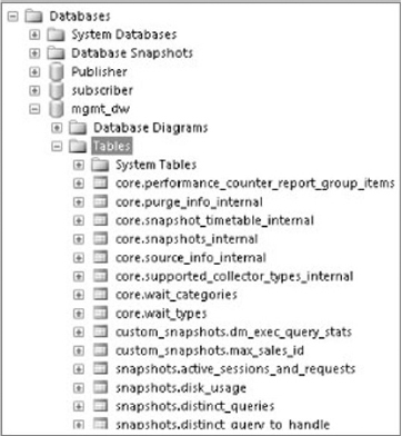
The table you created has some additional columns, not defined in the data you selected for the snapshot. These are database_name, collection_time, and snapshot_id. In addition, the collection time is stored in a datimeoffset column. This was a new data type in SQL Server 2008 and when queried, returns the date/time as a UTC time.
Following is the T-SQL to retrieve the data stored by the collection set you just created:
 -- Find the data you recorded
 -- Switch to the MDW
 use mgmt_dw
 go

 -- Query the custom snapshot
 select
* from custom_snapshots.max_sales_id
Table 12-6 shows the results of this query after the collector has been running for a few minutes with no inserts to the table.
TABLE 12-6: Custom Snapshots

To fully leverage the data stored in the Management Data Warehouse, consider creating SQL Server Reporting Services reports to display the data.
One of the best kept secrets in SQL Server is the standard reports that started shipping with the SQL Server 2005 Performance dashboard reports. Since then, each edition of SQL Server has added to the standard reporting capabilities, until today whence a comprehensive set of reports that provide a great deal of detailed information on what’s going on inside SQL Server has come about.
The standard reports are accessible through SQL Server Management Studio. Starting with the Server Node in SSMS, right-click the server node, then Reports, and then Standard Reports to see the list of reports for the SQL Server Instance. The list of standard reports for the server node is shown in Figure 12-33.

As you navigate through the various nodes in the Object Explorer, different reports are available at different key nodes. In some cases, no standard reports exist and just a custom report node that’s empty can be found. In other cases, such as when you select a specific database, a long list of standard reports is available. Figure 12-34 shows the standard reports for a database.
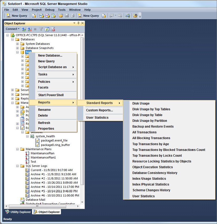
Unfortunately, these are not documented anywhere, so you have to find your own way around the various nodes in the Object Explorer by clicking nodes and looking in the Reports menu to see where there are any Standard Reports. Figure 12-35 shows one more location where there are standard reports, which is under Security ![]() Logins.
Logins.

All the monitoring discussed so far has been interactive in nature and has been based around activities that a single DBA executes against a small number of SQL Servers.
As DBAs must cover more and more databases, they need to change from an interactive monitoring mode to an exception-driven monitoring model. This is where the System Center suite, and specifically System Center Operations Manager comes in. System Center Operations Manager (SCOM) provides a product that delivers exception and performance monitoring that can gather a broad set of performance, health, and exception data from a large number of servers. SCOM then consolidates the data and presents a high-level rollup of your entire datacenter health.
This approach lets a relatively small team manage or operate a large number of servers, knowing that any time something needs to happen, an alert or exception will be raised that lets them react to the relevant activity.
SQL Server 2012 has a new management pack that integrates both with the current shipping version of System Center Operations Manager 2007, and also with the next version, System Center Operations Manager 2012.
SCOM 2012 provides some considerable enhancements to SCOM functionality that make the upgrade worthwhile. These are primarily the new dashboards that provide a consolidated view of SQL Server health.
SQL SERVER BEST PRACTICE ANALYZER
The SQL Server Best Practice Analyzer is a tool introduced around the SQL Server 2005 time frame to help you know if your SQL Server instance meets currently accepted best practices. It was originally a stand-alone tool developed by the SQL Server Release Services team but has since evolved into a set of rules implemented in the Microsoft Baseline Configuration Analyzer (MBCA) framework.
SQL Server Best Practice Analyzer (BPA) is a stand-alone tool installed to each instance on which you want to run it. Once you install it, you then run the BPA and point it at a given SQL instance, provide credentials for it to connect, and it scans the SQL Instance and compares its configuration with the set of rules included in that version of the SQL BPA.
Any exceptions to the rules are reported in the output, and each exception will include some basic text, and a link to an online resource providing more information about the rule that was infringed.
Something important to remember about SQL BPA is that these are general purpose best practices, and in some cases it’s perfectly acceptable that your SQL Server instance doesn’t meet the relevant best practice. However every exception should be considered, and you should ensure that you understand why your instance doesn’t meet the relevant rule.
Something else to consider is that just because your instance doesn’t fire any exceptions does not mean that everything is fine. There are plenty of specific best practices that are not incorporated into the SQL BPA, so a clean report doesn’t necessarily mean you’re optimally configured. However it is a great place to start.
System Center Advisor (SCA) is the natural evolution of SQL Server Best Practice Analyzer. One of the challenges with SQL BPA is that the set of rules are encoded into each version for BPA that’s released, and knowledge about best practices can change more quickly than new versions can be released. SQL BPA is also a tool that needs to be manually executed on each server.
System Center Advisor is the result of a lot of effort by folks who work with SQL Server and the SQL teams within PSS to deliver a more effective tool for validating SQL Server configurations.
System Center Advisor is a cloud-based configuration monitoring tool that can continuously monitor a large number of servers and provide online analysis of the results. One of the benefits of being cloud-based is that new best practices can be incorporated into the validation checks quickly, and with no activity on you, the end user’s part. The System Center Advisor team can introduce a new rule with minimal effort, and every server being monitored by SCA can immediately gain the benefit of being checked against the new rule.
Monitoring SQL Server regularly and gathering performance data is key to helping identify performance problems. Increasingly, today’s DBAs need to cover more systems than ever before and must spread their net widely. The tools and techniques introduced in this chapter help the DBAs do that to move from a hands-on approach to an event-driven approach.
Performance Monitor enables the DBA to monitor resource usage for a server, and helps troubleshoot performance issues with server and SQL resource usage.
The SQL Server Dynamic Management Views and Functions provide a deep insight into what’s going on inside SQL Server, and the samples provided help illustrate how to use some of the DMVs and DMFs to troubleshoot specific issues.
The SQL Trace architecture with SQL Profiler, SQL Trace, and now Distributed Replay provide tools for capturing, analyzing, and replaying SQL Server events.
Event Notifications provides a framework to execute actions outside SQL Server asynchronously in response to events occurring inside the server.
Extended Events provides a scalable framework for capturing data when specific events occur within SQL Server. This is a powerful framework that enables complex data collection to assist with troubleshooting SQL Server issues.
Data Collection sets, the Management Data Warehouse, and Utility MDW are a mechanism to collect performance related data and store it in a data warehouse. The Data Collector framework is a powerful way to store large amounts of performance data in a data warehouse for analysis should a performance issue occur, or just for trend analysis to see how load and performance is changing over time.
The System Center Operations Manager and the SQL Server 2012 Management Pack provide a central management interface for a data center operations team to monitor the health of hundreds of SQL Servers, and react to critical events when they occur.
SQL Server Best Practice Analyzer tells you when your SQL Server instance is in compliance with the established Best Practices.
System Center Advisor provides a cloud based service for best practices and for patch and update checking to help you keep your SQL Servers current with the very latest knowledge around SQL Server Best Practices.
In the next chapter you learn how to performance tune T-SQL.