Chapter 11
Optimizing SQL Server 2012
WHAT’S IN THIS CHAPTER
- Benefits to Optimizing Application Performance
- Using Partitioning and Compression to Improve Performance
- Tuning I/O, CPU, and Memory to Increase the Speed of Query Results
Since the inception of SQL Server 7.0, the database engine has been enabled for self-tuning and managing. With the advent of SQL Server 2012, these concepts have reached new heights. When implemented on an optimized platform (as described in Chapter 10, “Configuring the Server for Optimal Performance”) with a properly configured SQL Server instance that has also been well maintained, SQL Server 2012 remains largely self-tuning and healing. This chapter introduces and discusses the SQL Server 2012 technologies needed to accomplish this feat.
There are many ways to squeeze more performance out of your SQL Server, and it is a good idea to make sure the application is running optimally. Therefore, the first order of business for scaling SQL Server 2012 on the Windows Server platform is optimizing the application. The Pareto Principle, which states that only a few vital factors are responsible for producing most of the problems in scaling such an application, is reflected in this optimization. If the application is not well written, getting a bigger hammer only postpones your scalability issues, rather than resolving them. Tuning an application for performance is beyond the scope of this chapter.
The goal of performance tuning SQL Server 2012 is to minimize the response time for each SQL statement and increase system throughput. This can maximize the scalability of the entire database server by reducing network-traffic latency, and optimizing disk I/O throughput and CPU processing time.
Defining a Workload
A prerequisite to tuning any database environment is a thorough understanding of basic database principles. Two critical principles are the logical and physical structure of the data and the inherent differences in the application of the database. For example, different demands are made by an online transaction processing (OLTP) environment than are made by a decision support (DSS) environment. A DSS environment often needs a heavily optimized I/O subsystem to keep up with the massive amounts of data retrieval (or reads) it performs. An OLTP transactional environment needs an I/O subsystem optimized for more of a balance between read-and-write operations.
In most cases, SQL Server testing to scale with the actual demands on the application while in production is not possible. As a preferred practice, you need to set up a test environment that best matches the production system and then use a load generator such as Quest Benchmark Factory or Idera SQLscaler to simulate the database workload of the targeted production data-tier environment. This technique enables offline measuring and tuning the database system before you deploy it into the production environment.
Further, the use of this technique in a test environment enables you to compartmentalize specific pieces of the overall solution to be tested individually. As an example, using the load-generator approach enables you to reduce unknowns or variables from a performance-tuning equation by addressing each component on an individual basis (hardware, database, and application).
System Harmony Is the Goal
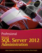
Scaling an application and its database is dependent on the harmony of the memory, disk I/O, network, and processors, as shown in Figure 11-1. A well-designed system balances these components and should enable the system (the application and data tiers) to sustain a run rate of greater than 80 percent processor usage. Run rate refers to the optimal CPU utilization when the entire system is performing under heavy load. When a system is balanced properly, this can be achieved as all sub-systems are performing efficiently.
Of these resource components, a processor bottleneck on a well-tuned system (applicationdatabase) is the least problematic to diagnose because it has the simplest resolution: add more processors or upgrade the processor speed/technology. There are, however, increased licensing costs associated with adding more processors and CPU cores.
THE SILENT KILLER: I/O PROBLEMS
Customers often complain about their SQL Server performance and point to the database because the processors aren’t that busy. After a discussion and a little elbow grease, frequently the culprit is an I/O bottleneck. The confusion comes from the fact that disk I/O is inversely proportional to CPU. In other words, over time, the processors wait for outstanding data requests queued on an overburdened disk subsystem. This section is about laying out the SQL Server shell or container on disk and configuring it properly to maximize the exploitation of the hardware resources. Scaling any database is a balancing act based on moving the bottleneck to the least affected resource.
SQL Server I/O Process Model
Windows Server 2008 with the SQL Server 2012 storage engine work together to mask the high cost of a disk I/O request. The Windows Server I/O Manager handles all I/O operations and fulfills all I/O (read or write) requests by means of scatter-gather or asynchronous methods. Scatter-gather refers to the process of gathering data from, or scattering data into, the disk or the buffer. For examples of scatter-gather or asynchronous methods, refer to SQL 2012 Books Online (BOL) under “I/O Architecture.”
The SQL Server storage engine manages when disk I/O operations are performed, how they are performed, and the number of operations that are performed. However, the Windows operating system (I/O Manager Subsystem) performs the underlying I/O operations and provides the interface to the physical media. SQL Server 2012 is only supported on Windows Server 2008 R2. For Windows 2008 R2 details, see www.microsoft.com/en-us/server-cloud/windows-server/default.aspx and select Editions under the Overview heading for edition specifics.
The job of the database storage engine is to manage or mitigate as much of the cost of these I/O operations as possible. For instance, the database storage engine allocates much of its virtual memory space to a data buffer cache. This cache is managed via cost-based analysis to ensure that memory is optimized to efficiently use its memory space for data content — that is, data frequently updated or requested is maintained in memory. This benefits the user’s request by performing a logical I/O and avoiding expensive physical I/O requests.
Database File Placement
SQL Server stores its database on the operating system files — that is, physical disks or Logical Unit Numbers (LUNs) surfaced from a disk array. The database is made up of three file types: a primary data file (MDF), one or more secondary data files (NDF), and transaction log files (LDF).
In SQL Server 2012, as in some previous versions, the use of MDF, NDF, and LDF file extensions is optional.
Database file location is critical to the I/O performance of the Database Management System (DBMS). Using a fast and dedicated I/O subsystem for database files enables it to perform most efficiently. As described in Chapter 10 “Configuring the Server for Optimal Performance,” available disk space does not equate to better performance. Rather, the more, faster physical drives there are, (or LUNs), the better your database I/O subsystem can perform. You can store data according to usage across data files and filegroups that span many physical disks. A filegroup is a collection of data files used in managing database data-file placement.
To maximize the performance gain, make sure you place the individual data files and the log files all on separate physical LUNs. You can place reference archived data or data that is rarely updated in a read-only filegroup. This read-only file group can then be placed on slower disk drives (LUNs) because it is not used very often. This frees up disk space and resources so that the rest of the database may perform better.
tempdb Considerations
Since database file location is so important to I/O performance, you need to consider functional changes to tempdb when you create your primary data-file placement strategy. The reason for this is that tempdb performance has a rather large impact on system performance because it is the most dynamic database on the system and needs to be the quickest.
Like all other databases, tempdb typically consists of a primary data and log files. tempdb is used to store user objects and internal objects. It also has two version stores. A version store is a collection of data pages that hold data rows required to support particular features that use row versioning. These two version stores are as follows:
- Row versions generated by data modification transactions in tempdb that use snapshot or read committed row versioning isolation levels
- Row versions in tempdb generated by data modification transactions for features such as online index operations, Multiple Active Result Sets (MARS), and AFTER triggers
Beginning with SQL Server 2005 and continuing in SQL Server 2012, tempdb has added support for the following large set of features that create user and internal objects or version stores:
- Query
- Triggers
- Snapshot isolation and read committed snapshots
- Multiple Active Result Sets (MARS)
- Online index creation
- Temporary tables, table variables, and table-valued functions
- DBCC Check
- Large Object (LOB) parameters
- Cursors
- Service Broker and event notification
- XML and Large Object (LOB) variable
- Query notifications
- Database mail
- Index creation
- User-defined functions
As a result, placing the tempdb database on a dedicated and extremely fast I/O subsystem can ensure good performance. A great deal of work has been performed on tempdb internals to improve scalability.
Consider reading BOL under “Capacity Planning for tempdb” for additional information and functionality details regarding tempdb usage. This can be found at: http://msdn.microsoft.com/en-us/library/ms345368.aspx.
When you restart SQL Server, tempdb is the only database that returns to the original default size of 8MB or to the predefined size set by the administrator. It can then grow from there based on usage requirements. During the autogrow operation, threads can lock database resources during the database-growth operation, affecting server concurrency. To avoid timeouts, the autogrow operation should be set to a growth rate that is appropriate for your environment. In general, the growth rate should be set to a number that will allow the file to grow in less than 2 minutes.
You should do at least some type of capacity planning for tempdb to ensure that it’s properly sized and can handle the needs of your enterprise system. At a minimum, perform the following:
1. Take into consideration the size of your existing tempdb.
2. Monitor tempdb while running the processes known to affect tempdb the most. The following query outputs the five executing tasks that make the most use of tempdb:
SELECT top 5 * FROM sys.dm_db_session_space_usage
ORDER BY (user_objects_alloc_page_count + internal_objects_alloc_page_count) DESC
3. Rebuild the index of your largest table online while monitoring tempdb. Don’t be surprised if this number turns out to be two times the table size because this process now takes place in tempdb.
Following is a recommended query that needs be run at regular intervals to monitor tempdb size. It is recommended that this is run every week, at a minimum. This query identifies and expresses tempdb space used, (in kilobytes) by internal objects, free space, version store, and user objects:
select sum(user_object_reserved_page_count)*8 as user_objects_kb,
    sum(internal_object_reserved_page_count)*8 as internal_objects_kb,
    sum(version_store_reserved_page_count)*8  as version_store_kb,
    sum(unallocated_extent_page_count)*8 as freespace_kb
from sys.dm_db_file_space_usage
where database_id = 2
The output on your system depends on your database setup and usage. The output of this query might appear as follows:
user_objects_kb      internal_objects_kb  version_store_kb     freespace_kb
-------------------- -------------------- -------------------- ---------------
256                  640                  0                    6208
If any of these internal SQL Server objects or data stores run out of space, tempdb will run out of space and SQL Server will stop. For more information, please read the BOL article on tempdb disk space that can be found here: http://msdn.microsoft.com/en-us/library/ms176029.aspx.
Taking into consideration the preceding results, when configuring tempdb, the following actions need to be performed:
- Pre-allocate space for tempdb files based on the results of your testing, but leave autogrow enabled in case tempdb runs out of space to prevent SQL Server from stopping.
- Per SQL Server instance, as a rule of thumb, create one tempdb data file per CPU or processor core, all equal in size up to a maximum of eight data files.
- Make sure tempdb is in simple recovery model, which enables space recovery.
- Set autogrow to a fixed size of approximately 10 percent of the initial size of tempdb.
- Place tempdb on a fast and dedicated I/O subsystem.
- Create alerts that monitor the environment by using SQL Server Agent or Microsoft System Center Operations Manager with SQL Knowledge Pack to ensure that you track for error 1101 or 1105 (tempdb is full). This is crucial because the server stops processing if it receives those errors. Right-click SQL Server Agent in SQL Server Management Studio and fill in the dialog, as shown in Figure 11-2. Moreover, you can monitor the following counters using Windows System Performance Monitor:
- SQLServer:Databases: Log File(s) Size(KB): Returns the cumulative size of all the log files in the database.
- SQLServer:Databases: Data File(s) Size(KB): Returns the cumulative size of all the data files in the database.
- SQLServer:Databases: Log File(s) Used (KB): Returns the cumulative used size of all log files in the database. A large active portion of the log in tempdb can be a warning sign that a long transaction is preventing log cleanup.
- Use instant database file initialization. If you are not running the SQL Server (MSSQLSERVER) Service account with admin privileges, make sure that the SE_MANAGE_VOLUME_NAME permission has been assigned to the service account. This feature can reduce a 15-minute file-initialization process to approximately 1 second for the same process.

Another great tool is the sys.dm_db_task_space_usage DMV, which provides insight into tempdb’s space consumption on a per-task basis. Keep in mind that once the task is complete, the counters reset to zero. In addition, you should monitor the per disk Avg. Sec/Read and Avg. Sec/Write as follows:
- Less than 10 milliseconds (ms) = Very good
- Between 10–20 ms = Borderline
- Between 20–50 ms = Slow, needs attention
- Greater than 50 ms = Serious IO bottleneck
If you have large tempdb usage requirements, read the Q917047, “Microsoft SQL Server I/O subsystem requirements for tempdb database” at http://support.microsoft.com/kb/917047 or look in SQL Server 2012 Books Online (BOL) for “Optimizing tempdb Performance.”
Hopefully this section has impressed upon you that in SQL Server 2012, more capacity planning is required to optimize tempdb for performance.
Simply stated, partitioning is the breaking up of a large object, such as a table, into smaller, manageable pieces. A row is the unit on which partitioning is based. Unlike DPVs, all partitions must reside within a single database.
Partitioning has been around for a while. This technology was introduced as a distributed partitioned view (DPV) during the SQL 7.0 launch. This feature received a lot of attention because it supported the ability to use constraints with views. This provided the capability for the optimizer to eliminate partitions (or tables) joined by a union of all statements on a view. These partitions could also be distributed across servers using linked servers.
However, running queries against a DPV on multiple linked servers could be slower than running the same query against tables on the same server due to the network overhead. As systems have become increasingly faster and more powerful, the preferred method has become to use the SQL Server capability to partition database tables and their indexes over filegroups within a single database. This type of partitioning has many benefits over DPV, such as being transparent to the application (meaning no application code changes are necessary). Other benefits include database recoverability, simplified maintenance, and manageability.
Although this section discusses partitioning as part of performance-tuning and as a way to present a path to resolve I/O problems, partitioning is first and foremost a manageability and scalability tool. In most situations, implementing partitioning also offers performance improvements as a byproduct of scalability.
You can perform several operations only on a partitioned table including the following:
- Switch partition data into or out of a table
- Merge partition range
- Split partition range
These benefits are highlighted throughout this section.
Partitioning is supported only in SQL Server 2012 Enterprise and Developer Editions.
Why Consider Partitioning?
There are a variety of reasons that you may have large tables. When these tables (or databases) reach a certain size, it becomes difficult to perform activities such as database maintenance, backup, or restore operations that consume a lot of time. Environmental issues such as poor concurrency due to a large number of users on a sizable table result in lock escalations, which translates into further challenges. If archiving the data is not possible because of regulatory compliance needs, independent software vendor (ISV) requirements, or cultural requirements, partitioning is most likely the tool for you. If you are still unsure whether to implement partitioning, run your workload through the Database Tuning Advisor (DTA), which makes recommendations for partitioning and generates the code for you. Chapter 15 “Replication,” covers the DTA, which you can find under the “Performance Tools” section of the Microsoft SQL Server 2012 program menu.
Various chapters in this book cover partitioning to ensure you learn details in their appropriate contexts.
Following is a high-level process for partitioning:
1. Create a partition function to define a data-placement strategy.
2. Create filegroups to support the partition function.
3. Create a partition scheme to define the physical data distribution strategy (map the function data to filegroups).
4. Create a table or index on the partition function.
5. Enjoy redirected queries to appropriate resources.
After implementation, partitioning can positively affect your environment and most of your processes. Make sure you understand this technology to ensure that every process benefits from it. The following list presents a few processes that may be affected by partitioning your environment:
- Database backup and restore strategy (support for partial database availability)
- Index maintenance strategy (rebuild), including index views
- Data management strategy (large insert or table truncates)
- End-user database workload
- Concurrency:
- Parallel partition query processing: In SQL Server 2005, if the query accessed only one table partition, then all available processor threads could access and operate on it in parallel. If more than one table partition were accessed by the query, then only one processor thread was allowed per partition, even when more processors were available. For example, if you have an eight-processor server and the query accessed two table partitions, six processors would not be used by that query. In SQL Server 2012, parallel partition processing has been implemented whereby all available processors are used in parallel to satisfy the query for a partition table. The parallel feature can be enabled or disabled based on the usage requirements of your database workload.
- Table partition lock: escalation strategy.
- Enhanced distribution or isolated database workloads using filegroups
Creating a Partition Function
A partition function is your primary data-partitioning strategy. When creating a partition function, the first order of business is to determine your partitioning strategy. Identifying and prioritizing challenges is the best way to decide on a partitioning strategy. Whether it’s to move old data within a table to a slower, inexpensive I/O subsystem, enhance database workload concurrency, or simply maintain a large database, identifying and prioritizing is essential. After you select your strategy, you need to create a partitioning function that matches that strategy.
Remember to evaluate a table for partitioning because the partition function is based on the distribution of data (selectivity of a column and the range or breadth of that column). The range supports the number of partitions by which the table can be partitioned. There is a product limit of 15,000 partitions per table. This range should also match up with the desired strategy — for example, spreading out (or partitioning) a huge customer table by customer last name or by geographical location for better workload management may be a sound strategy. Another example of a sound strategy may be to partition a table by date for the purpose of archiving data based on date range for a more efficient environment.
You cannot implement user-defined data types, alias data types, timestamps, images, XML, varchar(max), nvarchar(max), or varbinary(max) as partitioning columns.
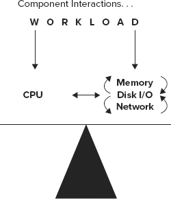
Take for example a partition of a trouble-ticketing system for a telephone company. When a trouble ticket is generated based on an outage, it is submitted to the database. At this point, many activities are initiated: Technicians are dispatched, parts are replaced or reordered, and service can be rerouted within the network. Service-level agreements (SLAs) are monitored and escalations are initiated. All these activities take place because of the trouble ticket. In this system, the activities table and ticketing table have hot spots, as shown in Figure 11-3.
In Figure 11-3, the information marked as Hot is the new or recent data, which is only relevant or of interest during the outage. The information marked as Read-Only and Read-Mostly is usually used for minor analysis during postmortem processes and then for application reporting. Eventually, the data becomes obsolete and should be moved to a warehouse. Unfortunately, because of internal regulatory requirements, this database must be online for 7 years. Partitioning this environment can provide sizable benefits. Under a sliding-window scenario (explained in the “Creating a Partition Scheme” section later in this chapter), every month (or quarter) a new partition would be introduced to the environment as a retainer for the current (Hot) data for the tickets and activities tables. As part of this process, a partition with data from these tables that is older than 7 years would also be retired.
As described earlier, there is a one-to-many relationship between tickets and activities. Although obvious size differences exist between these tables, you need to put them through identical processes. This enables you to run processes that affect resources shared by and limited to these objects. To mitigate the impact of doing daily activities such as backups and index maintenance on all this data, these tables will be partitioned based on date ranges. You can create a right partition function based on the ticketdate column, as outlined in Listing 11-1 (if you execute the following statement, remove the line breaks):
LISTING 11-1: CreatePartitionFunction
CREATE PARTITION FUNCTION
PFL_Years (datetime)
AS RANGE RIGHT
FOR VALUES (
'20050101 00:00:00.000', '20070101 00:00:00.000',
'20090101 00:00:00.000', '20110101 00:00:00.000',
'20120101 00:00:00.000')
SQL Server rounds time to .003 seconds, meaning that a time of .997 would be rounded up to 1.0 second.
- The leftmost partition is the first partition and includes all values less than '20050101 00:00:00.000'.
- The boundary value '20050101 00:00:00.000' is the start of the second partition, and this partition includes all values greater than or equal to '20050101 00:00:00.000' but less than '20070101 00:00:00.000'.
- The boundary value '20070101 00:00:00.000' is the start of the third partition, and this partition includes all values greater than or equal to '20070101 00:00:00.000' but less than '20090101 00:00:00.000'.
- The boundary value '20090101 00:00:00.000' is the start of the fourth partition and this partition includes all values greater than or equal to '20090101 00:00:00.000' but less than '20110101 00:00:00.000'.
- The boundary value '20110101 00:00:00.000' is the start of the fifth partition and includes all values greater than or equal to '20110101 00:00:00.000' but less than '20120101 00:00:00.000'.
- Finally, the boundary value ‘20120101 00:00:00.000’ is the start of the sixth partition, and this partition consists of all values greater than '20120101 00:00:00.000'.
The range partition function specifies the boundaries of the range. The left or right keyword specifies to which side of each boundary value interval, left or right, the boundary_value belongs, when interval values are sorted by the Database Engine in ascending order from left to right. If this keyword is not specified, left is the default. There can be no holes in the partition domain; all values must be obtainable. In this code sample, all transactions must fall within a date specified by the sample value range.
Creating Filegroups
You should create filegroups to support the strategy set by the partition function. As a best practice, user objects should be created and mapped to a filegroup outside of the primary filegroup, leaving the primary filegroup for system objects. This ensures database availability if an outage occurs that affects the availability of any filegroup outside of the primary filegroup.
To continue with this example exercise, you need to create filegroups CY04, CY06, CY08, CY10, CY11, and CY12 in the database before creating the partition scheme.
Creating a Partition Scheme
A partition scheme is what maps database objects such as a table to a physical entity such as a filegroup, and then to a file. There are definitely backup, restore, and data-archival considerations when making this decision. (These are discussed in Chapter 17, “Backup and Recovery.”) Listing 11-2 maps the partition functions or dates to individual filegroups. The partition scheme depends on the PFL_Years partition function to be available from the earlier example.
LISTING 11-2: CreatePartitionScheme1
CREATE PARTITION SCHEME CYScheme
AS
PARTITION PFL_Years
TO ([CY04], [CY06], [CY08], [CY10], [CY11], [CY12])
This supports the placement of filegroups on individual physical disk subsystems. Such an option also supports the capability to move old data to an older, inexpensive I/O subsystem and to reassign the new, faster I/O subsystem to support Hot data (CY12). When the older data has been moved to the inexpensive I/O subsystem, filegroups can be marked as read-only. When this data has been backed up, it no longer needs to be part of the backup process. SQL Server automatically ignores these filegroups as part of index maintenance.
The other option for a partition-function scheme enables the mapping of the partition scheme to map the partition function to a single filegroup. Listing 11-3 maps the partition function to the default filegroup.
This code will fail if you have not created the PFL_Years partition function.
LISTING 11-3: CreatePartitionScheme2
CREATE PARTITION SCHEME CYScheme2
AS
PARTITION PFL_Years
TO ([Default], [Default], [Default], [Default], [Default], [Default])
Partitioning enables the ability to delete or insert gigabytes of data on a 500+ GB partitioned table with a simple metadata switch (in seconds) provided that the delete or insert is based on the partitioned column. The process used to accomplish this is called sliding window. On a non-partitioned table, this process would take hours because of lock escalation and index resynchronization. However, using a partitioned table with the sliding-window process consists of the following three steps:
1. An empty target table or partitioned table is created outside of the source data partitioned table.
2. The source data partitioned table is switched with the empty target.
3. At the conclusion of this process, the data is now in the target table and can be dropped.
This process could be repeated in reverse to insert a new partition with data into this source partitioned table as the repository for the Hot data. Again, the only impact to the source partitioned table is a brief pause while a schema-lock is placed during the partition swaps, which can take a few seconds. This switch process can be performed only on partitions within the same filegroup. Implementation details and best practices are covered later in this chapter and in upcoming chapters.
Creating Tables and Indexes
As Listing 11-4 shows, the syntax for creating a table is accomplished as it has always been. The only exception is that it is created on a partition schema instead of a specific or default filegroup. SQL Server 2012 provides the capability to create tables, indexes, and indexed views on partition schemes. This supports the distribution of database objects across several filegroups. This is different from the existing capability to create an entire object within a filegroup (which is still available in SQL Server 2012).
LISTING 11-4: CreateTables
CREATE TABLE [dbo].[Tickets]
(     [TicketID] [int] NOT NULL,
       [CustomerID] [int] NULL,
       [State] [int] NULL,
        [Status] [tinyint] NOT NULL,
        [TicketDate] [datetime] NOT NULL
        CONSTRAINT TicketYear
        CHECK ([TicketDate] >= '20050101 00:00:00.000'
AND [TicketDate] < '20120101 00:00:00.000'))
 ON CYScheme (TicketDate)
GO

CREATE TABLE [dbo].[Activities]
(     [TicketID] [int] NOT NULL,
       [ActivityDetail] [varchar] (255) NULL,
      [TicketDate] [datetime] NOT NULL,
       [ActivityDate] [datetime] NOT NULL
       CONSTRAINT ActivityYear
       CHECK ([ActivityDate] >= '20050101 00:00:00.000'
AND [ActivityDate] < '20120101 00:00:00.000'))
ON CYScheme (TicketDate)
GO
The following sections cover two areas of best practices when creating indexes: index alignment and storage alignment.
Index Alignment
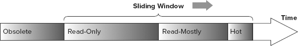
An aligned index uses an equivalent partition function and includes the same partitioning columns as its table (as shown in Figure 11-4). These indexes actually don’t need to use the identical partition function or scheme, but there must be a one-to-one correlation of data-to-index entries within a partition.
A benefit derived from index alignment is the ability to switch partitions in or out of a table with a simple metadata operation. In Listing 11-4, you can programmatically add a new partition for the new month (or current month) and delete the outgoing month from the table as part of the 7-year cycle.
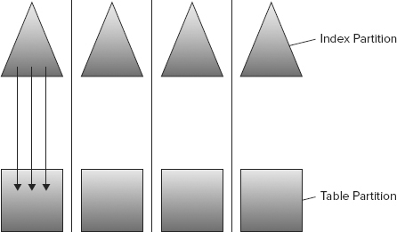
Storage Alignment
Index alignment is the first requirement of a storage-aligned solution. There are two options for storage alignment. The big differentiator is the ability to use the same partition scheme, or a different one, as long as both tables and indexes have an equal number of partitions. The first option, as shown in Figure 11-5, demonstrates a storage-aligned solution with the index and relevant data in distinct and dedicated filegroups. If a query to compare data in CY08 and CY06 is executed on an aligned index and data, the query is localized to the aligned environment. This benefits users working in other table partitions isolated from the ongoing work within these two partitions.

Figure 11-6 shows the same query executed on a different architecture. Because of the alignment of index and data, the query is still localized but runs in parallel on both the relevant index and data partitions. This would still benefit users working in other partitions isolated from the ongoing work within these four partitions.

Additional benefits derived from storage alignment are partial database availability and piecemeal database restores. For instance, in Listing 11-2, the CY08 partition could be offline, and the application would still be processing trouble tickets. This would occur regardless of which partition went down, as long as the primary filegroup that contains the system-tables information (as is the best practice) and the partition that contains the current month’s data are online. Considerations that affect query parallelism of this environment are discussed later in the CPU Considerations section of this chapter.
Listing 11-5 is an example of a SQL script for partitioning operations on a table using the AdventureWorks database. For simplicity in this example, all the partitions are placed on the primary file group, but in a real-life scenario, to achieve I/O performance benefits, partitions may be placed on different filegroups, which are then placed on different physical disk drives.
1. First, create the partition function:
LISTING 11-5: StorageAlignment
USE AdventureWorks;
CREATE PARTITION FUNCTION [OrderDateRangePFN](datetime)
AS RANGE RIGHT
FOR VALUES (N'2009-01-01 00:00:00', N'2010-01-01 00:00:00',
N'2011-01-01 00:00:00', N'2012-01-01 00:00:00'),
2. Then create the partition scheme:
CREATE PARTITION SCHEME [OrderDatePScheme]
AS PARTITION [OrderDateRangePFN]
TO ([Primary], [Primary], [Primary], [Primary], [Primary]);
3. Now, create two tables: SalesOrderHeader is the partitioned table and SalesOrderHeaderOLD is the nonpartitioned table.
4. Load data into the SalesOrderHeader table and then create clustered indexes on both tables.
5. Finally, apply a check constraint to the SalesOrderHeaderOLD table to allow the data to switch into the SalesOrderHeader partitioned table:
CREATE TABLE [dbo].[SalesOrderHeader](
  [SalesOrderID] [int] NULL,
  [RevisionNumber] [tinyint] NOT NULL,
  [OrderDate] [datetime] NOT NULL,
  [DueDate] [datetime] NOT NULL,
  [ShipDate] [datetime] NULL,
  [Status] [tinyint] NOT NULL
) ON [OrderDatePScheme]([OrderDate]);

CREATE TABLE [dbo].[SalesOrderHeaderOLD](
  [SalesOrderID] [int] NULL,
  [RevisionNumber] [tinyint] NOT NULL,
  [OrderDate] [datetime] NOT NULL  ,
  [DueDate] [datetime] NOT NULL,
  [ShipDate] [datetime] NULL,
  [Status] [tinyint] NOT NULL);

INSERT INTO SalesOrderHeader SELECT [SalesOrderID],[RevisionNumber],
[OrderDate],[DueDate],[ShipDate],[Status] FROM SALES.[SalesOrderHeader];

CREATE CLUSTERED INDEX SalesOrderHeaderCLInd
ON SalesOrderHeader(OrderDate) ON OrderDatePScheme(OrderDate);

 CREATE CLUSTERED INDEX SalesOrderHeaderOLDCLInd ON
SalesOrderHeaderOLD(OrderDate);

ALTER  TABLE [DBO].[SalesOrderHeaderOLD]  WITH CHECK  ADD CONSTRAINT
[CK_SalesOrderHeaderOLD_ORDERDATE] CHECK  ([ORDERDATE]>=('2011-01-01
00:00:00') AND [ORDERDATE]<('2012-01-01 00:00:00'));
Before you start to do table partition operations, you should verify that you have data in the partitioned table and no data in the nonpartitioned table. The following query returns which partitions have data and how many rows:
SELECT $partition.OrderDateRangePFN(OrderDate) AS 'Partition Number',
min(OrderDate) AS 'Min Order Date',
max(OrderDate) AS 'Max Order Date',
count(*) AS 'Rows In Partition'
FROM SalesOrderHeader
GROUP BY $partition.OrderDateRangePFN(OrderDate);
You should also verify that no data has been inserted into the SalesOrderHeaderOLD nonpartitioned table; this query should return no data:
SELECT * FROM [SalesOrderHeaderOLD]
To simply switch the data from partition 4 into the SalesOrderHeaderOLD table, execute the following command:
ALTER TABLE SalesOrderHeader
SWITCH PARTITION 4 TO SalesOrderHeaderOLD;
To switch the data from SalesOrderHeaderOLD back to partition 4, execute the following command:
ALTER TABLE SalesOrderHeaderOLD
SWITCH TO SalesOrderHeader PARTITION 4;
To merge a partition range, execute the following command:
ALTER PARTITION FUNCTION OrderDateRangePFN()
MERGE RANGE ('2011-01-01 00:00:00'),
You may want to split a partition range. The split range area should be empty of data because if data were available, SQL Server would need to physically (I/O) move the data across the range. For a large table, the data movement can take time and resources. Therefore, if the range is not empty, the split is not instantaneous. To split a range, you must add a new filegroup for the range before splitting it, like so:
ALTER PARTITION SCHEME OrderDatePScheme NEXT USED [Primary];
ALTER PARTITION FUNCTION OrderDateRangePFN()
SPLIT RANGE ('2013-01-01 00:00:00'),
This section discussed what partitioning is and why it should be considered as a performance option or as a manageability and scalability feature. You ran through the steps to create the partition function and the partition scheme. Remember that filegroup creation needs to be performed prior to these steps. The section ended with an outline of the various options used when creating tables and indexes that use the partition scheme. Next you will learn about Data Compression and how it pertains to increasing efficiency in a database.
SQL Server 2012 data compression brings enhancements in storage and performance benefits. Reducing the amount of disk space that a database occupies reduces the overall data files storage footprint and offers increase in throughput with the following improvements:
- Better I/O utilization, as more data is read and written per page
- Better memory utilization, as more data will fit in the buffer cache
- Reduction in page latching, as more data will fit in each page
It is true that disk space is becoming less expensive. However, implementation of a high-performance database system requires a high-performing disk system or Storage Area Network (SAN) or Network Attached Storage (NAS), which is not inexpensive. In addition, this may require additional storage for high availability, backups, QA, and test environments. Overall, it lowers SQL Server 2012’s total cost of ownership, making it more competitive.
Before implementing data compression, you must consider the trade-off between I/O and CPU. To compress and uncompress data requires CPU processing utilization, so it would not be recommended for a system that is CPU-bound. However, it would benefit a system that is more I/O-bound. Additionally, keep in mind that accessing the compressed data requires CPU processing work, and if this data is highly selected, there is a CPU performance penalty. Data compression makes most sense on data that is older and less queried. As a simple example, with a large partitioned table, the older partitions that are less queried may be compressed, whereas the highly volatile partitions are not. You can compress volatile data, but you must consider the costs versus benefits for your database workload, and the capacity of your hardware to support it with the goal to achieve the highest throughput.
Data compression is only available in SQL Server 2012 Enterprise and Developer Editions.
You can use data compression on the following database objects:
- Tables (but not system tables)
- Clustered indexes
- Non-clustered indexes
- Index views
- Partitioned tables and indexes where each partition can have a different compression setting
Row Compression
SQL Server 2012 implements row and page data compression. The data compression ratio depends on the schema and data distribution, where compression stores fixed-value data types in a variable format — that is, a 4-byte column with a 1-byte value can be compressed to a size of 1 byte. A 1-byte column with a 1-byte value has no compression, but NULL or 0 values take no bytes. Compression does take a few bits of metadata overhead to store per value. For example, an Integer data type column storing a 1-byte value can have a 75 percent compression ratio. To create a new compressed table with row compression, use the CREATE TABLE command, as follows:
 USE AdventureWorks
 GO
 CREATE TABLE [Person].[AddressType_Compressed_Row](
  [AddressTypeID] [int] IDENTITY(1,1) NOT NULL,
  [Name] [dbo].[Name] NOT NULL,
  [rowguid] [uniqueidentifier] ROWGUIDCOL  NOT NULL,
  [ModifiedDate] [datetime] NOT NULL,
 )
 WITH (DATA_COMPRESSION=ROW)
 GO
To change the compression setting of a table, use the ALTER TABLE command:
 USE AdventureWorks
 GO
 ALTER TABLE Person.AddressType_Compressed_Row REBUILD
 WITH (DATA_COMPRESSION=ROW)
 GO
Page Compression
Page compression includes row compression and then implements two other compression operations:
- Prefix compression: For each page and each column, a prefix value is identified that can be used to reduce the storage requirements. This value is stored in the Compression Information (CI) structure for each page. Then, repeated prefix values are replaced by a reference to the prefix stored in the CI.
- Dictionary compression: Searches for repeated values anywhere in the page, which are replaced by a reference to the CI.
When page compression is enabled for a new table, new inserted rows are row compressed until the page is full, and then page compression is applied. If afterward there is space in the page for additional new inserted rows, they are inserted and compressed; if not, the new inserted rows go onto another page. When a populated table is compressed, the indexes are rebuilt. Using page compression, nonleaf pages of the indexes are compressed using row compression. To create a new compressed table with page compression, use the following commands:
 USE AdventureWorks
 GO
 CREATE TABLE [Person].[AddressType_Compressed_Page](
  [AddressTypeID] [int] IDENTITY(1,1) NOT NULL,
  [Name] [dbo].[Name] NOT NULL,
  [rowguid] [uniqueidentifier] ROWGUIDCOL  NOT NULL,
  [ModifiedDate] [datetime] NOT NULL,
 )
 WITH (DATA_COMPRESSION=PAGE)
 GO
To change the compression setting of a table, use the ALTER TABLE command:
 USE AdventureWorks
 GO
 ALTER TABLE Person.AddressType_Compressed_Page REBUILD
 WITH (DATA_COMPRESSION=PAGE)
 GO
Moreover, on a partitioned table or index, compression can be applied or altered on individual partitions. The following code shows an example of applying compression to a partitioned table and index:
 USE AdventureWorks
 GO

 CREATE PARTITION FUNCTION [TableCompression](Int)
 AS RANGE RIGHT
 FOR VALUES (1, 10001, 12001, 16001);
 GO

 CREATE PARTITION SCHEME KeyRangePS
 AS
 PARTITION [TableCompression]
 TO ([Default], [Default], [Default], [Default], [Default])
 GO

 CREATE TABLE PartitionTable
 (KeyID int,
 Description varchar(30))
 ON KeyRangePS (KeyID)
 WITH
 (
 DATA_COMPRESSION = ROW ON PARTITIONS (1),
 DATA_COMPRESSION = PAGE ON PARTITIONS (2 TO 4)
 )
 GO

 CREATE INDEX IX_PartTabKeyID
  ON PartitionTable (KeyID)
 WITH (DATA_COMPRESSION = ROW ON PARTITIONS(1),
 DATA_COMPRESSION = PAGE ON PARTITIONS (2 TO 4 ) )
 GO
Table partition operations on a compression partition table have the following behaviors:
- Splitting a partition: Both partitions inherit the original partition setting.
- Merging partitions: The resultant partition inherits the compression setting of the destination partition.
- Switching partitions: The compression setting of the partition and the table to switch must match.
- Dropping a partitioned clustered index: The table retains the compression setting.
In addition, data compression can be managed from SQL Server 2012 Management Studio in Object Explorer by choosing the table or index to data compress. For example, to compress a table, follow these steps:
1. Choose the table and then right-click. From the pop-up menu, choose Storage ![]() Manage Compression.
Manage Compression.
2. On the Data Compression Wizard that opens, click Next, and in the Select Compression Type dialog of the Data Compression Wizard, select the Compression Type drop-down to change the compression (None, Row, or Page). Figure 11-7 shows the Select Compression Type dialog.
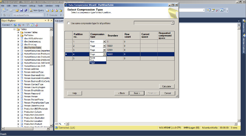
3. After making a Compression Type change, to see the estimated space savings, click the Calculate button. Then, click Next to complete the wizard.
Estimating Space Savings
Prior to enabling data compression, you can evaluate the estimated compression cost-savings. For example, if a row is more than 4KB and the whole value precision is always used for the data type, there may not be much compression savings. The sp_estimate_data_compression_savings stored procedure creates a sample data set in tempdb and evaluates the compression space savings, returning the estimated table and sample savings. It can evaluate tables, clustered indexes, nonclustered indexes, index views, and table and index partitions for either page or row compression. Moreover, this stored procedure can estimate the size of a compressed table, index, or partition in the uncompressed state. This stored procedure performs the same cost-saving calculation that was performed by the Data Compression Wizard shown in Figure 11-7 when clicking the Calculate button.
The syntax of the sp_estimate_data_compression_savings stored procedure follows:
 sp_estimate_data_compression_savings
 [ @schema_name = ] 'schema_name'
 , [ @object_name = ] 'object_name'
 , [@index_id = ] index_id
 , [@partition_number = ] partition_number
 , [@data_compression = ] 'data_compression'
 [;]
In this code:
- @schema_name is the name of the schema that contains the object.
- @object_name is the name of the table or index view that the index is on.
- @index_id is the ID number of the index. Specify NULL for all indexes in a table or view.
- @partition_number is the partition number of the object; it can be NULL or 1 for nonpartitioned objects.
- @data_compression is the type of compression to evaluate; it can be NONE, ROW, or PAGE.
Figure 11-8 shows an example of estimating the space savings for the SalesOrderDetail table in the AdventureWorks database using page compression.

As shown in the result information in Figure 11-8:
- index_id identifies the object. In this case, 1 = clustered index (includes table); 2 and 3 are nonclustered indexes.
- Size_with_current_compression_setting is the current size of the object.
- Size_with_requested_compression_setting is the compressed size of the object
In this example, the clustered index, including the table, is 9952KB but when page-compressed, it is 4784KB, saving a space of 5168KB.
Monitoring Data Compression
For monitoring data compression at the SQL Server 2012 instance level, two counters are available in the SQL Server:Access Method object that is found in Windows Performance Monitor:
- Page compression attempts/sec counts the number of page compression attempts per second.
- Pages compressed/sec counts the number of pages compressed per second.
The sys.dm_db_index_operational_stats dynamic management function includes the page_compression_attempt_count and page_compression_success_count columns which are used to obtain page compression statistics for individual partitions. It is important to take note of these metrics because failures of attempted compression operations waste system resources. If the ratio of attempts to successes gets too high then there may be performance impacts that could be avoided by removing compression. In addition, the sys.dm_db_index_physical_stats dynamic management function includes the compressed_page_count column, which displays the number of pages compressed per object and per partition.
To identify compressed objects in the database, you can view the data_compression column (0=None, 1=Row, 2=Page) of the sys.partitions catalog view. From SQL Server 2012 Management Studio in Object Explorer, choose the table and right-click; then, from the pop-up menu choose Storage ![]() Manage Compression for the Data Compression Wizard. For detailed information on data compression, refer to “Data Compression” in SQL Server 2012 Books Online, which can be found here: http://msdn.microsoft.com/en-us/library/cc280449(v=SQL.110).aspx.
Manage Compression for the Data Compression Wizard. For detailed information on data compression, refer to “Data Compression” in SQL Server 2012 Books Online, which can be found here: http://msdn.microsoft.com/en-us/library/cc280449(v=SQL.110).aspx.
Data Compression Considerations
When deciding whether to use data compression, keep the following items in mind:
- Data compression is available with SQL Server 2008 Enterprise and Developer Editions only.
- Enabling and disabling table or clustered index compression can rebuild all non-clustered indexes.
- Data compression cannot be used with sparse columns.
- Large objects (LOB) that are out-of-row are not compressed.
- Non-leaf pages in indexes are compressed using only row compression.
- Non-clustered indexes do not inherit the compression setting of the table.
- When you drop a clustered index, the table retains those compression settings.
- Unless specified, creating a clustered index inherits the compression setting of the table.
A word of caution for high-availability systems: Changing the compression setting may generate extra transaction log operations.
The challenge in building a large Symmetric Multiprocessing (SMP) system is that, because processors have increased performance through technology enhancements and the use of increasingly larger caches, the performance gains achieved through leveraging these caches are significant. Consequently, you need to cache relevant data whenever possible to enable processors to have relevant data available and resident in their caches. Chip and hardware vendors have attempted to capitalize on this phenomenon through expansion of the processor and system cache.
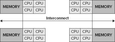
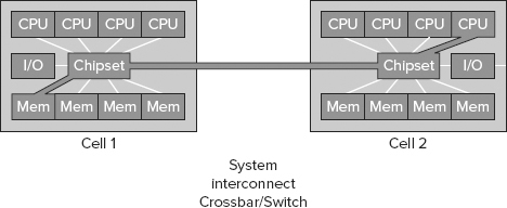
As a result, new system architectures such as cellular multiprocessing (CMP), CC-NUMA (see Figure 11-9), and NUMA (noncache coherent) are now available in the market. Although this has been successful, it has produced two challenges: the need to manage data locally and cache coherency.
With Windows 2008 and SQL Server 2012, SQL Server supports hot-add CPU, whereby CPUs can be dynamically added while the server is online. The system requirements to support hot-add CPU are as follows:
- Hardware support for hot-add CPU.
- Supported by the 64-bit edition of Windows Server 2008 Datacenter or the Windows Server 2008 Enterprise Edition for Itanium-Based Systems operating system.
- Supported by SQL Server 2012 Enterprise Edition.
- SQL Server 2012 must not be configured for soft NUMA. For more information about soft NUMA, search for the following topics online: “Understanding Non-Uniform Memory Access” and “How to Configure SQL Server to Use Soft-NUMA.”
Once you have met these requirements, execute the RECONFIGURE command to have SQL Server 2012 recognize the new dynamically added CPU.
Cache Coherency
For reasons of data integrity, only one processor can update any piece of data at a time; other processors that have copies in their caches can have their local copy “invalidated” and thus must be reloaded. This mechanism is referred to as cache coherency, which requires that all the caches are in agreement regarding the location of all copies of the data and which processor currently has permission to perform the update. Supporting coherency protocols is one of the major scaling problems in designing big SMPs, particularly if there is a lot of update traffic. Cache coherency protocols were better supported with the introduction of NUMA and CMP architectures.
SQL Server 2012 has been optimized to take advantage of NUMA advancements exposed by both Windows and the hardware itself. As discussed in the “Memory Considerations and Enhancements” section, SQLOS is the technology that the SQL Server leverages to exploit these advances.
Affinity Mask
The affinity mask configuration option restricts a SQL Server instance to running on a subset of the processors. If SQL Server 2012 runs on a dedicated server, allowing SQL Server to use all processors can ensure best performance. In a server consolidation or multiple-instance environment, for more predictable performance, SQL Server may be configured on dedicated hardware resources that affinitize processors by SQL Server instance.
SQL Server Processor Affinity Mask
SQL Server’s mechanism for scheduling work requests is handled through a data structure concept called a scheduler. The scheduler is created for each processor assigned to SQL Server through the affinity mask configuration setting at startup. Worker threads (a subset of the max worker threads configuration setting) are dynamically created during a batch request and are evenly distributed between each CPU node and load-balanced across its schedulers (see Figure 11-10).
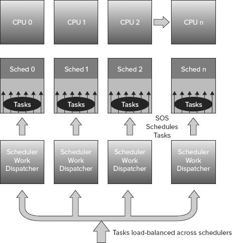
Incoming connections are assigned to the CPU node. SQL Server assigns the batch request to a task or tasks, and the tasks are managed across schedulers. At any given time, only one task can be scheduled for execution by a scheduler on a processor. A task is a unit of work scheduled by the SQL Server. This architecture guarantees an even distribution of the hundreds, or in many cases, thousands of connections that can result from a large deployment.
Default SQL Server Work Scheduling
The default setting for affinity mask is 0, which enables the Windows scheduler to schedule and move schedulers across any available processor within a CPU node to execute its worker threads. SQL Server 2012 in this configuration has its processes controlled and scheduled by the Windows scheduler. For example, suppose a client requests a connection and the connection is accepted. If no threads are available, then one is dynamically created and associated with a task. The work assignments from the scheduler to the processors are managed through the Windows scheduler, which has its work distributed among all processors within a CPU node. This is the preferred method of execution, as Windows load-balances the schedulers evenly on all processors.
SQL Server Work Scheduling Using Affinity Mask
You can use the affinity mask configuration setting to assign a subset of the available processors to the SQL Server process. SQL Server worker threads are scheduled preemptively by the scheduler. A worker thread continues to execute on its processor until it is forced to wait for a resource, such as locks or I/O, to become available. If the time slice expires, the thread voluntarily yields, at which time the scheduler selects another worker thread to begin execution. If it cannot proceed without access to a resource such as disk I/O, it sleeps until the resource is available. When access to that resource is available, the process is placed on the run queue before being put back on the processor. When the Windows kernel transfers control of the processor from an executing process to another that is ready to run, this is referred to as a context switch.
Context Switching
Context switching is expensive because of the associated housekeeping required to move from one running thread to another. Housekeeping refers to the maintenance of keeping the context or the set of processor register values and other data that describes the process state. The Windows kernel loads the context of the new process, which then starts to execute. When the process taken off the processor next runs, it resumes from the point at which it was taken off the processor. This is possible because the saved context includes the instruction pointer. In addition to this user mode time, context switching can take place in the Windows operating system (OS) for privileged mode time.
The total processor time is equal to the privileged mode time plus the user mode time.
Privileged Mode
Privileged mode is a processing mode designed for operating system components and hardware-manipulating drivers. It enables direct access to hardware and all memory. Privileged time includes time-servicing interrupts and deferred process calls (DPCs).
User Mode
User mode is a restricted processing mode designed for applications such as SQL Server, Exchange, and other application and integral subsystems. The goal of performance tuning is to maximize user mode processing by reducing privileged mode processing. This can be monitored with the Processor: % Privileged Time counter, which displays the average busy time as a percentage of the sample time. A value above 15 percent may indicate that a disk array is being heavily used or that there is a high volume of network traffic requests. In some rare cases, a high rate of privileged time might even be attributed to a large number of interrupts generated by a failing device.
Priority Boost
The Priority Boost option is an advanced option under SQL Server. If you are using the sp_configure system stored procedure to change the setting, you can change Priority Boost only when Show Advanced Options is set to 1. The setting takes effect after the server is restarted. By enabling the Priority Boost option, SQL Server runs at a priority base of 13 in the Windows System scheduler, rather than its default of 7. On a dedicated server, this might improve performance, although it can also cause priority imbalances between SQL Server functions and operating system functions, leading to instability. Improvements in SQL Server 2012 and Windows make the use of this option unnecessary.
Priority boost should not be used when implementing failover clustering.
SQL Server Lightweight Pooling
Context switching can often become problematic. In most environments, context switching should be less than 1,000 per second per processor. The SQL Server lightweight pooling option provides relief for this by enabling tasks to use NT “fibers,” rather than threads, as workers.
A fiber is an executable unit that is lighter than a thread and operates in the context of user mode. When lightweight pooling is selected, each scheduler uses a single thread to control the scheduling of work requests by multiple fibers. A fiber can be viewed as a “lightweight thread,” which under certain circumstances takes less overhead than standard worker threads to context switch. The number of fibers is controlled by the Max Worker Threads configuration setting.
Common Language Runtime (CLR) execution is not supported when lightweight pooling is enabled. Make sure to disable the option: “clr enabled” when lightweight pooling is desired.
Max Degree of Parallelism (MAXDOP)
By default, the MAXDOP value is set to 0, which enables SQL Server to consider all processors when creating an execution plan. In most systems, a MAXDOP setting equivalent to the number of cores (to a maximum of 8) is recommended. This limits the overhead introduced by parallelization. In some systems, based on application-workload profiles, it is even recommended that you set this value to 1 (including for SAP and Siebel). This can prevent the query optimizer from choosing parallel query plans. Using multiple processors to run a single query is not always desirable in an OLTP environment, although it is desirable in a data warehousing environment.
In SQL Server 2012, you should assign query hints to individual queries to control the degree of parallelism. If, however, a third party application is generating the query, consider using resource pools to control this.
Partitioned table parallelism is also affected by the MAXDOP setting. Returning to Listing 11-5, a thread can be leveraged across each partition. Had the query been limited to a single partition, multiple threads would be spawned up to the MAXDOP setting.
Affinity I/O Mask
The affinity I/O mask feature, as shown in Figure 11-11, was introduced with SP1 of SQL Server 2000. This option defines the specific processors on which SQL Server I/O threads can execute. The affinity I/O mask option has a default setting of 0, indicating that SQL Server threads are allowed to execute on all processors. The performance gains associated with enabling the affinity I/O mask feature are achieved by grouping the SQL threads that perform all I/O tasks (no-data cache retrievals — specifically, physical I/O requests) on dedicated resources. This keeps I/O processing and related data in the same cache systems, maximizing data locality and minimizing unnecessary bus traffic.

When using affinity masks to assign processor resources to the operating system, either SQL Server processes (non-I/O) or SQL Server I/O processes, you must be careful not to assign multiple functions to any individual processor.
You should consider SQL I/O affinity when there is high privileged time on the processors that is not affinitized to SQL Server. For example, consider a 32-processor system running under load with 30 of the 32 processors affinitized to SQL Server, leaving two processors to the Windows OS and other non-SQL activities. If the Processor: % Privileged time is high (greater than 15 percent), SQL I/O affinity can be configured to help reduce the privileged-time overhead in the processors assigned to SQL Server.
The following steps outline the SQL I/O affinity procedure for determining what values to set:
1. Add I/O capability until there is no I/O bottleneck (disk queue length has been eliminated) and all unnecessary processes have been stopped.
2. Add a processor designated to SQL I/O affinity.
3. Measure the CPU utilization of these processors under heavy load.
4. Increase the number of processors until the designated processors are no longer peaked. For a non-SMP system, select processors that are in the same cell node.
MEMORY CONSIDERATIONS AND ENHANCEMENTS
Because memory is fast relative to disk I/O, using this system resource effectively can have a large impact on the system’s overall ability to scale and perform well.
SQL Server 2012 memory architecture and capabilities vary greatly from those of previous versions of SQL Servers. Changes include the ability to consume and release memory-based, internal-server conditions dynamically using the AWE mechanism. In SQL Server 2000, all memory allocations above 4GB were static. Additional memory enhancements include the introduction of hierarchical memory architecture to maximize data locality and improve scalability by removing a centralized memory manager. SQL Server 2012 has resource monitoring, dynamic management views (DMVs), and a common caching framework. All these concepts are discussed throughout this section.
Tuning SQL Server Memory
The following performance counters are available from the System Performance Monitor. The SQL Server Cache Hit Ratio signifies the balance between servicing user requests from data in the data cache and having to request data from the I/O subsystem. Accessing data in RAM (or data cache) is exponentially faster than accessing the same information from the I/O subsystem; thus, the wanted state is to load all active data in RAM. Unfortunately, RAM is a limited resource. A wanted cache hit ratio average should be well over 90 percent. This does not mean that the SQL Server environment would not benefit from additional memory. A lower number signifies that the system memory or data cache allocation is below the wanted size.
Another reliable indicator of instance memory pressure is the SQL Server:Buffer Manager:Page-life-expectancy (PLE) counter. This counter indicates the amount of time that a buffer page remains in memory, in seconds. The ideal number for PLE varies with the size of the RAM installed in your particular server and how much of that memory is used by the plan cache, Windows OS, and so on. The rule of thumb nowadays is to calculate the ideal PLE number for a specific server using the following formula: MaxSQLServerMemory(GB) x 75. So, for a system that has 128GB of RAM and has a MaxServerMemory SQL setting of 120GB, the “minimum PLE before there is an issue” value is 9000. This can give you a more realistic value to monitor PLE against than the previous yardstick of 300. Be careful not to under-allocate total system memory because it forces the operating system to start moving page faults to a physical disk. A page fault is a phenomenon that occurs when the operating system goes to a physical disk to resolve memory references. The operating system may incur some paging, but when excessive paging takes places, it uses disk I/O and CPU resources, which can introduce latency in the overall server, resulting in slower database performance. You can identify a lack of adequate system memory by monitoring the Memory: Pages/sec performance counter. It should be as close to zero as possible because a higher value indicates that more hard-paging is taking place, as can happen when backups are taking place.
SQL Server 2012 has several features that should help with this issue. With Windows Server 2008, SQL Server 2012 has support for hot-add memory, a manager framework, and other enhancements. The SQL Server operating system (SQLOS) layer is the improved version of the User Mode Scheduler (UMS), now simply called scheduler. Consistent with its predecessor, SQLOS is a user-mode cooperative and on-demand thread-management system. An example of a cooperative workload is one that yields the processor during a periodic interval or while in a wait state, meaning that if a batch request does not have access to all the required data for its execution, it requests its data and then yields its position to a process that needs processing time.
SQLOS is a thin layer that sits between SQL Server and Windows to manage the interaction between these environments. It enables SQL Server to scale on any hardware. This was accomplished by moving to a distributed model and creating an architecture that would foster locality of resources to aid in getting rid of global resource management bottlenecks. The challenge with global resource management is that in large hardware design, global resources cannot keep up with the demands of the system, slowing overall performance. Figure 11-12 highlights the SQLOS components that perform thread scheduling and synchronization, perform SQL Server memory management, provide exception handling, and host the Common Language Runtime (CLR).

The goal of this environment is to empower the SQL Server platform to exploit all of today’s hardware innovation across the X86, X64, and IA64 platforms. SQLOS was built to bring together the concepts of data locality, support for dynamic configuration, and hardware workload exploitation. This architecture also enables SQL Server 2012 to better support both Cache Coherent Non-Uniform Memory Access (CC-NUMA), Interleave NUMA (NUMA hardware with memory that behaves like an SMP system), Soft-NUMA architecture (registry-activated, software-based emulated NUMA architecture used to partition a large SMP system), and large SMP systems, by affinitizing memory to a few CPUs.
The architecture introduces the concept of a memory node, which is one hierarchy between memory and CPUs. There is a memory node for each set of CPUs to localize memory and its content to these CPUs. On an SMP architecture, a memory node shares memory across all CPUs, whereas on a NUMA architecture, a memory node per NUMA node exists. As shown in Figure 11-13, the goal of this design is to support SQL Server scalability across all hardware architectures by enabling the software to adapt to or emulate various hardware architectures.

Schedulers are discussed later in this chapter, but for the purposes of this discussion, they manage the work executed on a CPU.
Memory nodes share the memory allocated by Max Server Memory, setting evenly across a single memory node for SMP system and across one or more memory nodes for NUMA architectures. Each memory node has its own lazy writer thread that manages its workload based on its memory node. As shown in Figure 11-14, the CPU node is a subset of memory nodes and provides for logical grouping for CPUs.

A CPU node is also a hierarchical structure designed to provide logical grouping for CPUs. The purpose is to localize and load-balance related workloads to a CPU node. On an SMP system, all CPUs would be grouped under a single CPU node, whereas on a NUMA-based system, there would be as many CPU nodes as the system supported. The relationship between a CPU node and a memory node is explicit. There can be many CPU nodes to a memory node, but there can never be more than one memory node to a CPU node. Each level of this hierarchy provides localized services to the components that it manages, resulting in the capability to process and manage workloads in such a way as to exploit the scalability of whatever hardware architecture SQL Server runs on. SQLOS also enables services such as dynamic affinity, load-balancing workloads, dynamic memory capabilities, Dedicated Admin Connection (DAC), and support for partitioned resource management capabilities.
SQL Server 2012 leverages the common caching framework (also part of SQLOS) to achieve fine-grain control over managing the increasing number of cache mechanisms (Cache Store, User Store, and Object Store). This framework improves the behavior of these mechanisms by providing a common policy that can be applied to internal caches to manage them in a wide range of operating conditions. For additional information about these caches, refer to SQL Server 2012 Books Online.
SQL Server 2012 also features a memory-tracking enhancement called the Memory Broker, which enables the tracking of OS-wide memory events. Memory Broker manages and tracks the dynamic consumption of internal SQL Server memory. Based on internal consumption and pressures, it automatically calculates the optimal memory configuration for components such as buffer pool, optimizer, query execution, and caches. It propagates the memory configuration information back to these components for implementation. SQL Server 2012 also supports dynamic management of conventional, locked, and large-page memory, as well as the hot-add memory feature mentioned earlier.
The Windows policy Lock Pages in Memory is granted by default to the local administrative accounts but can be explicitly granted to other user accounts. To ensure that memory runs as expected, it needs this privilege to enable SQL Server to manage which pages are flushed out of memory and which pages are kept in memory.
Hot-add memory provides the ability to introduce additional memory in an operational server without taking it offline. In addition to OEM vendor support, Windows Server 2008 and SQL Server 2012 Enterprise Edition are required to support this feature. Although a sample implementation script is provided in the following section, refer to BOL for additional implementation details.
64-bit Versions of SQL Server 2012
As SQL Server 2012 is only found in an x64 variety, you are in luck. SQL Server 2012 64-bit supports 1TB of RAM, and all of it is native addressable memory so there’s no need for /3GB or /PAE switches in your boot.ini file. The mechanism used to manage AWE memory in 32-bit systems can be used to manage memory on 64-bit systems. Specifically, this mechanism ensures that SQL Server manages what is flushed out of its memory. To enable this feature, the SQL Server service account requires the Lock Pages in Memory privilege. To grant this access to the SQL Service account, use the Windows Group Policy tool (gpedit.msc) and perform the following steps:
1. On the Start menu, click Run. In the Open box, type gpedit.msc. The Group Policy dialog box opens.
2. On the Group Policy console, expand Computer Configuration, and then expand Windows Settings.
3. Expand Security Settings, and then expand Local Policies.
4. Select the User Rights Assignment folder.
5. The policies will be displayed in the details pane. In this pane, double-click Lock pages in memory.
6. In the Local Security Policy Setting dialog box, click Add.
7. In the Select Users or Groups dialog box, add the account that will be used to run sqlservr.exe.
You need to identify the type of application driving the database and verify that it can benefit from a large SQL Server data-cache allocation. In other words, is it memory-friendly? Simply stated, a database that does not need to keep its data in memory for an extended length of time cannot benefit from a larger memory allocation. For example, a call-center application in which no two operators handle the same customer’s information and where no relationship exists between customer records has no need to keep data in memory because data won’t be reused. In this case, the application is not deemed memory-friendly; thus, keeping customers’ data in memory longer than required would not benefit performance. Another type of inefficient memory use occurs when an application stores excessive amounts of data, beyond what is required by an operation — for example, a table scan. This type of operation suffers from the high cost of data invalidation. Larger amounts of data than are necessary are read into memory and thus must be flushed out.
Data Locality
Data locality is the concept of having all relevant data available to the processor on its local NUMA node while it’s processing a request. All memory within a system is available to any processor on any NUMA node. This introduces the concepts of near memory and far memory. Near memory is the preferred method because it is accessed by a processor on the same NUMA node. As shown in Figure 11-15, accessing far memory is expensive because the request must leave the NUMA node and traverse the system interconnect crossbar to get the NUMA node that holds the required information in its memory.
The cost of accessing objects in far memory versus near memory is often threefold or more. Data locality is managed by the system itself and the way to mitigate issues with it is to install additional memory per NUMA node.
Max Server Memory
When max server memory is kept at the default dynamic setting, SQL Server acquires and frees memory in response to internal and external pressure. SQL Server uses all available memory if left unchecked, so the max server memory setting is strongly recommended. The Windows OS needs some memory to function, so a value of 8GB to 16GB less than the total system memory should be configured. Please refer to the following table for configuration guidelines:
| TOTAL SYSTEM MEMORY (GB) | OS RESERVED MEMORY (GB) | MAX SQL SERVER MEMORY (GB) |
| 16 | 4 | 12 |
| 32 | 6 | 26 |
| 64 | 8 | 56 |
| 128 | 16 | 112 |
| 256 | 16 | 240 |
Index Creation Memory Option
The index creation memory setting, as shown in Figure 11-16, determines how much memory can be used by SQL Server for sort operations during the index-creation process. The default value of 0 enables SQL Server to automatically determine the ideal value. In conditions in which index creation is performed on large tables, pre-allocating space in memory enables a faster index-creation process.
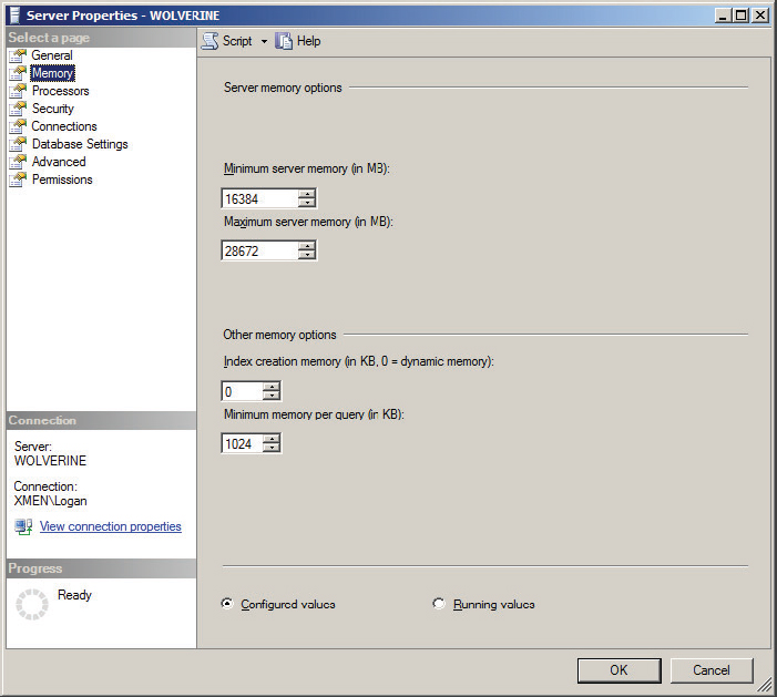
After memory is allocated, it is reserved exclusively for the index-creation process, and values are set in KB of memory. The index creation setting should only be changed when issues are observed.
Minimum Memory per Query
You can use the Minimum Memory per Query option to improve the performance of queries that use hashing or sorting operations. SQL Server automatically allocates the minimum amount of memory set in this configuration setting. The default Minimum Memory per Query option setting is equal to 1024KB (refer to Figure 11-16). It is important to ensure that the SQL Server environment has the minimum amount of query memory available. However, in an environment with high query-execution concurrency, if this setting is configured too high, SQL Server waits for a memory allocation to meet the minimum memory level before executing a query.
Resource Governor is a SQL Server technology that limits the amount of resources that can be allocated to each database workload from the total resources available to SQL Server 2012. When enabled, Resource Governor classifies each incoming session and determines to which workload group the session belongs. Each workload group is then associated to a resource pool that limits those groups of workloads. Moreover, Resource Governor protects against runaway queries on the SQL Server and unpredictable workload execution, and sets workload priority. For Resource Governor to limit resources, it must differentiate workloads as follows:
- Classifies incoming connections to route them to a specific workload group
- Monitors resource usage for each workload group
- Pools resources to set limits on CPU and memory to each specific resource pool
- Identifies workloads and groups them together to a specific pool of resources
- Sets workload priority within a workload group
The constraints on Resource Governor are as follows:
- It applies only to the SQL Server Relational Engine and not to Analysis Services, Report Services, or Integration Services.
- It cannot monitor resources between SQL Server instances. However, you can use Windows Resource Manager (part of Windows) to monitor resources across Windows processes, including SQL Server.
- It can limit CPU bandwidth and memory.
- A typical OLTP workload consists of small and fast database operations that individually take a fraction of CPU time and may be too miniscule to enable Resource Governor to apply bandwidth limits.
The Basic Elements of Resource Governor
The main elements of Resource Governor include resource pools, workload groups, and classification support, explained in the following sections.
Resource Pools
The resource pools are the physical resources of the SQL Server. During SQL Server installation, two pools are created: internal and default. The resources that can be managed are min and max CPU and min and max memory. By default, the Resource Governor is disabled; to enable it, use the ALTER RESOURCE GOVERNOR RECONFIGURE command. You can disable it again with the command ALTER RESOURCE GOVERNOR DISABLE.
The internal pool is used for SQL Server’s own internal functions. It contains only the internal workload group; it cannot be altered, and it is not restricted.
The default pool is the predefined user resource pool. It contains the default workload group and can contain user-defined workload groups. It can be altered but cannot be created or dropped.
You can create user-defined pools using the CREATE RESOURCE POOL DDL statement or by using SQL Server Management Studio. Moreover, you can modify a pool by using the ALTER RESOURCE POOL command, and delete it by using the DROP RESOURCE POOL command. You may define any number of resource pools as you want, up to a maximum of 20. This includes the internal and default pools.
The following syntax creates a resource pool for Resource Governor:
CREATE RESOURCE POOL pool_name
[ WITH
          ( [ MIN_CPU_PERCENT = value ]
     [ [ , ] MAX_CPU_PERCENT = value ]
     [ [ , ] CAP_CPU_PERCENT = value ]
     [ [ , ] AFFINITY {SCHEDULER = AUTO | (Scheduler_range_spec) | NUMANODE = (NUMA_node_range_spec)}]      [ [ , ] MIN_MEMORY_PERCENT = value ]
     [ [ , ] MAX_MEMORY_PERCENT = value ] )
]  [;]
Please note that CAP_CPU_PERCENT and AFFINITY are new options available in SQL Server 2012. Please see the Books Online topic for more information which can be found here: http://msdn.microsoft.com/en-us/library/bb934024(v=SQL.110).aspx.
Workload Groups
A workload group is a container for similar sessions according to the defined classification rules and applies the policy to each session of the group. It also contains two predefined workload groups: internal and default. The internal workload group relates to the internal resource pool and cannot be changed. The default workload group is associated with the default resource pool and is the group used when no session classification user-defined function exists, when a classification failure occurs, or when a classification user-defined function returns NULL.
You can create the user-defined workload group by using the CREATE WORKLOAD GROUP command, modify it by using the ALTER WORKLOAD GROUP command, and drop it by using the DROP WORKLOAD GROUP command.
The following syntax creates a workload group for Resource Governor:
 CREATE WORKLOAD GROUP group_name
 [ WITH
     ( [ IMPORTANCE = { LOW | MEDIUM | HIGH } ]
            [ [ , ] REQUEST_MAX_MEMORY_GRANT_PERCENT = value ]
            [ [ , ] REQUEST_MAX_CPU_TIME_SEC = value ]
            [ [ , ] REQUEST_MEMORY_GRANT_TIMEOUT_SEC = value ]
            [ [ , ] MAX_DOP = value ]
            [ [ , ] GROUP_MAX_REQUESTS = value ] )
  ]
 [ USING { pool_name | "default" } ] [ ; ]
You can apply seven configuration settings to a workload group:
- Maximum memory allocation per request
- Maximum CPU time per request
- Resource time-out per request
- Relative importance setting per request
- Workgroup limit per number of requests
- Maximum degree of parallelism
- Specific resource pool
Classification
Resource Governor supports classifying incoming connections into existing workload groups. It supports system-wide provided rules and user-defined rules using connection-specific attributes. In the absence of a user-defined classification function, it can use the default workload group. After the user-defined classification function is registered with Resource Governor, the function is executed for every new connection, and the connection is routed to one of the existing workload groups to be limited by the resource pool. Only one user-defined classification function can be designated as a classifier; and after registering it, it takes effect after an ALTER RESOURCE GOVERNOR RECONFIGURE command is executed.
Resource Governor uses connection-specific functions such as HOST_NAME(), APP_NAME(), SUSER_NAME(), SUSER_SNAME(), IS_SRVROLEMEMBER() and IS_MEMBER() to identify each connection.
Figure 11-17 shows the components of Resource Governor and their relationships.
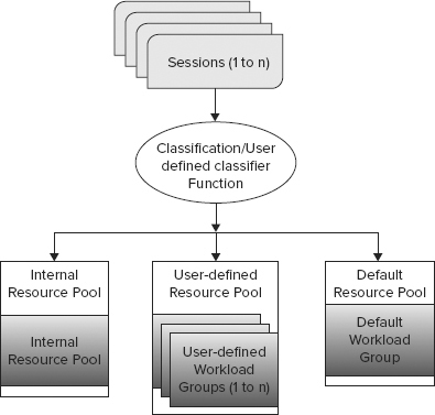
Following is a Resource Governor Implementation example that creates three resource pools to support the resource requirements for three different workload groups.
1. First, create three resource pools: adhoc, reports, and admin requests:
LISTING 11-6: ResourcePools
USE Master;
BEGIN TRAN;
CREATE RESOURCE POOL poolAdhoc with
( MIN_CPU_PERCENT = 10, MAX_CPU_PERCENT = 30,
MIN_MEMORY_PERCENT= 15, MAX_MEMORY_PERCENT= 25);

CREATE RESOURCE POOL poolReports with
( MIN_CPU_PERCENT = 20, MAX_CPU_PERCENT = 35,
MIN_MEMORY_PERCENT= 15,  MAX_MEMORY_PERCENT= 45);

CREATE RESOURCE POOL poolAdmin with
( MIN_CPU_PERCENT = 15, MAX_CPU_PERCENT = 25,
MIN_MEMORY_PERCENT= 15, MAX_MEMORY_PERCENT= 30);
2. Next, create three workload groups and associate them with the three resource pools:
CREATE WORKLOAD GROUP groupAdhoc using poolAdhoc;
CREATE WORKLOAD GROUP groupReports with (MAX_DOP = 8) using poolReports;
CREATE WORKLOAD GROUP groupAdmin using poolAdmin;
GO
3. Create a user-defined classification function that identifies each new session and routes it to one of the three workload groups. Any request that cannot be identified by the user-defined classification function is directed to the default workload group:
CREATE FUNCTION rgclassifier_v1() RETURNS SYSNAME
WITH SCHEMABINDING
AS
BEGIN
     DECLARE @grp_name AS SYSNAME
       IF (SUSER_NAME() = 'sa')
           SET @grp_name = 'groupAdmin'
       IF (APP_NAME() LIKE '%MANAGEMENT STUDIO%')
           OR (APP_NAME() LIKE '%QUERY ANALYZER%')
           SET @grp_name = 'groupAdhoc'
       IF (APP_NAME() LIKE '%REPORT SERVER%')
           SET @grp_name = 'groupReports'
     RETURN @grp_name
END;
GO
4. Next, the user-defined classification function needs to be registered to Resource Governor. All these operations are contained inside an explicit transaction. That’s a preventive measure so that if a user error occurs, it can be rolled back. In addition, only one user-defined classification function can be registered to the Resource Governor at any one time:
ALTER RESOURCE GOVERNOR WITH (CLASSIFIER_FUNCTION= dbo.rgclassifier_v1);
COMMIT TRAN;
5. Finally, to have these new changes take effect or to enable Resource Governor, run the following command:
ALTER RESOURCE GOVERNOR RECONFIGURE;
Using Resource Governor from SQL Server 2012 Management Studio
From inside SQL Server 2012 Management Studio in Object Explorer, Resource Governor is in the Management node. By default, Resource Governor is disabled. To enable it, right-click Resource Governor and then click Enable. Moreover, from Object Explorer inside the Management node, right-click Resource Governor, and then click Properties to add, delete, or modify properties of the resource pools and workload groups or to add or remove a user-defined classification function and enable Resource Governor. From the Resource Governor Properties dialog, you can see that two resource pools, Internal and Default, with two corresponding workload groups, are visible. These are created by SQL Server 2012 during installation. No classification function is available until one is created. If Resource Governor is enabled, it uses the default system-defined rules and the default pool, as configured in Figure 11-18.
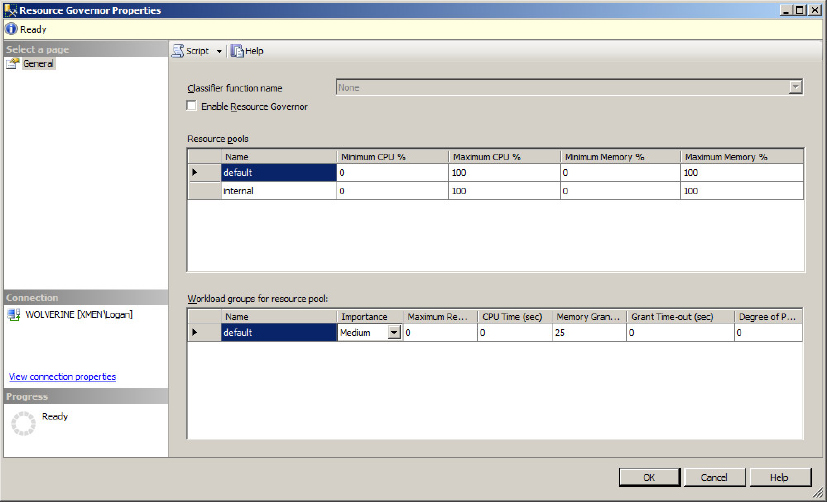
After running the script in Listing 11-6 to create the three user-defined resource pools, workload groups, and the user-defined classification function, and after enabling the Resource Governor, the properties should match what is shown in Figure 11-19.
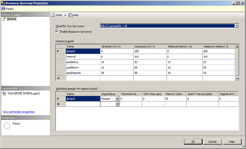
Monitoring Resource Governor
SQL Server 2012 includes two performance objects to collect workload group and pool statistics for each SQL Server instance:
- SQLServer: Resource Pool Stats for resource-specific statistics: Please see this article for more information: http://msdn.microsoft.com/en-us/library/cc645958(v=SQL.110).aspx
- SQLServer: Workload Group Stats for workload-specific statistics: Please see this article for more information: http://msdn.microsoft.com/en-us/library/cc627354(v=SQL.110).aspx
Moreover, there are Resource Governor Dynamic Management Views (DMVs) that return information specific to resource statistics, as indicated in the following table.
| RESOURCE GOVERNOR DYNAMIC MANAGEMENT VIEWS | DESCRIPTION |
| sys.dm_resource_governor_configuration | For current in-memory configuration state |
| sys.dm_resource_governor_resource_pools | For resource pool state, configuration, and statistics |
| sys.dm_resource_governor_workload_groups | For workload group statisticvs and in-memory configuration |
For more detailed information on Resource Governor, refer to SQL 2012 Books Online under “Resource Governor.” This can be found at: http://msdn.microsoft.com/en-us/library/bb933866(v=SQL.110).aspx.
There are many important points to consider when setting up and configuring SQL Server 2012. Database files (data and log files) should be placed on separate LUNs, which are made up of fast disks. tempdb should be placed on its own set of disks which should be the fastest possible. Partitioning can be used to increase performance and offers manageability advantages. Compression can be used to increase I/O performance but care needs to be taken not to overtax the CPU. CPU and memory can be tweaked from within SQL Server, but care must also be taken here not to use settings that are detrimental. Remember: test, test, test!
If you apply these lessons correctly, SQL Server 2012 is more than capable of tuning itself automatically to predictably provide the availability and performance to support the requirements of your enterprise.