
From images to mathematical models: intravoxel micromechanics for ceramics and polymers
K. Luczynski, A. Dejaco and C. Hellmich, Vienna University of Technology, Austria
V. Komlev, Russian Academy of Sciences, Russia
W. Swieszkowski, Warsaw University of Technology, Poland
Abstract:
We review here a recently developed method rooted in X-ray physics and continuum micromechanics, which allows for translation of data from computed tomography at micrometre resolution (known as microCT data) into finite element models. The method comprises two steps: first, the attenuation information contained in each voxel of a microCT image is converted into the voxel-specific material composition. Secondly, material composition information enters a micromechanics model representing the mechanical behaviour of the material’s microstructure within each and every voxel. Application of the method to both polymers and ceramics is followed by a brief future outlook.
Key words
micromechanics; microCT; polymer; hydroxyapatite; tissue engineering scaffold; finite element
10.1 Introduction
Computed tomography (CT) has become an indispensable tool in biomedical engineering. In particular at high resolutions with voxel size in the micrometre range, it is standardly used for characterization for both polymer and ceramic biomaterials. The impact of CT at micrometre resolution (microCT) has been revolutionary, enabling us to view internal sample details with unprecedented precision and in a non-destructive way. Typical corresponding image evaluation procedures comprise phase distinction through thresholding (Mastrogiacomo et al., 2004, 2005), as well as identification of pore size distribution and shapes, i.e. they are focusing on the topology of the investigated scaffold. The accuracy of microCT for scaffold materials was tested in a number of studies (Atwood et al., 2004; Mastrogiacomo et al., 2004; Cancedda et al., 2007). In addition, microCT images have been used as source for the generation of large finite element models of scaffolds (Jaecques et al., 2004), in order to learn more about their mechanical behaviour, in a procedure sometimes referred to as a ‘virtual mechanical experiment’. Therefore, all voxels are typically divided into ‘solid voxels’ (above a certain density threshold) and ‘pore voxels’ (below the same threshold), and the solid voxels are converted into finite elements, while the pore voxels are not further processed.
What remains, is the question on the mechanical properties of the matter filling the voxels. Standardly, they are just guessed, but in recent years, a more elegant and reliable method, rooted in X-ray physics (Crawley et al., 1988) and continuum micromechanics (Zaoui, 2002), has been proposed. In this chapter, we review this method based on the developments as reported in Hellmich et al. (2008), Scheiner et al. (2009), Dejaco et al. (2012), Luczynski et al. (2012) and Blanchard et al. (2013), and we show its application to both polymer and ceramic biomaterials. The method falls into two parts: first, the attenuation information contained in each voxel is converted into the voxel-specific material composition, in terms of voxel-specific volume fractions of the material’s elementary constituents. Secondly, the aforementioned volume fractions enter a micromechanics model representing the behaviour of the material’s microstructure within each voxel, delivering voxel-specific mechanical properties. Both steps will be developed in greater detail in the following sections of this chapter, first generally and then applied to ceramic and polymer biomaterials, respectively. Finally, typical mechanical features of ceramic and polymer tissue engineering scaffolds will be discussed, based on simulation results from intravoxel micromechanics-enhanced finite element models, built up according to the aforementioned two-step method.
10.2 Conversion of voxel-specific computed tomography (CT) data into material composition (volume fractions)
10.2.1 Fundamentals
The grey scale values (GV) assigned to each voxel of a CT image are linearly related to the voxel-specific X-ray attenuation coefficients μ,
μ=GV×a+b [10.1]
with proportionality constants a and b.
However, at a constant incident energy, chosen for a CT image, the attenuation coefficients of composite materials, like biological tissues and polymer- or ceramic-based biomaterials, are equal to the volume averages of the attenuation coefficients of their single constituents (Jackson and Hawkes, 1981; Crawley et al., 1988; Hellmich et al., 2008; Scheiner et al., 2009),
μ=Nc∑iμrfr [10.2]
where r numbers the Nc single constituents, μr is the attenuation coefficient of a voxel entirely filled by constituent r only, and fr is the volume fraction of constituent r, ∑Ncr=1fr=1![]() . This ‘mixture rule’ delivers reasonably accurate results, with an error of less than a few per cent (Jackson and Hawkes, 1981).
. This ‘mixture rule’ delivers reasonably accurate results, with an error of less than a few per cent (Jackson and Hawkes, 1981).
Specification of Eq. [10.1] for voxels filled by only one material constituent with attenuation coefficient μr = GVr × a + b, and use of these specifications in Eq. [10.2] yields an average rule for grey scale values
GV=Nc∑rGVrfr [10.3]
with GVr as the grey value related to a voxel which is entirely filled by constituent r. Frequently, values of GVr cannot be determined from the CT images alone, so that some ‘calibration process’ is needed. An interesting approach, without any use of phantoms, is based on relating the voxelspecific volume fraction to the voxel-specific mass density ρvox, through application of the mass density average rule,
ρvox=Nc∑rρrfr [10.4]
with ρr as the real mass density of the material constituent, which is standardly well known. Additionally, the average of the values for ρvox over the entire scanned object is identical to the apparent mass density ρapp of the scanned biomaterial scaffold, which is
1V∫Vρvox(x)dV=ρapp [10.5]
with x as the position vector of each voxel. Finally, combination of Eq. [10.3] with [10.5] may give access to the required value for GVr. In the following, this will be further developed for ceramics and polymers.
10.2.2 Application of CT-to-composition conversion technique to ceramic biomaterials
Based on the work of Dejaco et al. (2012), we consider here granules of hydroxyapatite (HA), which were prepared according to the processing route described in Komlev et al. (2002), where an aqueous gelatine solution with fine HA powder was dispersed in oil, and where subsequent stirring resulted in granule formation due to surface tension forces. Such spherical HA granules exhibit widely ranging diameters, from 50 to about 2000μm (see Fig. 10.1(a) for a scanning electron micrograph (SEM)). Within these globules, pores of two sizes are observed: the larger ones (‘micropores’) are in the order of one to several hundred micrometres, while the smaller ones (‘nanopores’) have a characteristic size of less than one micrometre.

A single granule with an approximate diameter of 1800 μm (Fig. 10.2) was investigated. This globule was μCT-scanned in a SKYSCAN 1172 μCT desktop machine. Appropriate machine settings, as described in more detail in (Dejaco et al., 2012), provided satisfactory image quality (Fig. 10.2). Within each voxel, two material ‘constituents’ occur: (i) solid HA and (ii) nanoporous air. The volume fraction of the latter is standardly called nanoporosity ϕnano; so that the grey value average rule, Eq. [10.3], can be specified to
GV=ϕnanoGVair+(1−ϕnano)GVHA [10.6]
with GVair as the grey value of an air-filled voxel, and GVHA as the grey value of a voxel which is totally filled by pure (dense) hydroxyapatite. Eq. [10.6] can be transformed, as to provide the (a priori unknown) voxel-specific nanoporosity ϕnano from the (a priori known) grey values GV, in the form
ϕnano(GV)=GV−GVHAGVair−GVHA [10.7]

However, the question remains as to how to determine the constituent-specific grey values GVair and GVHA · GVair = 100 can be identified from the ‘air peak’ of the grey value histogram of the investigated granule (Fig. 10.3): More precisely, we use the minimum value between the ‘air peak’ and the ‘solid peak’ in Fig. 10.3 as the threshold GVthr = 139, separating the pure ‘air voxels’ (with GV ≤ GVthr) from the ‘solid voxels’ (GV > GVthr), the latter containing a pure HA and some nanopores according to Eq. [10.7]. It follows
ϕnano(GV)=GV−GVHAGVair−GVHAforGV>GVthr [10.8]
and
ϕnano(GV)=1forGV≤GVthr [10.9]

None of the voxels of the (normalized) histogram of Fig. 10.3 is entirely filled with pure HA. This is because the single HA crystals as shown in Fig. 10.1(b) are much smaller than the voxel size of 3.49 μm. Hence, the value for GVHA cannot directly be retrieved from Fig. 10.3, and we need to find an alternative way to identify GVHA, which, according to the aforementioned considerations, is expected to be larger than 255. Therefore, we resort to the novel ‘calibration strategy’ sketched in Section 10.2.1. We consider, as additional quantities, the (known) mass and the (known) volume of investigated globule, as well as the (known) mass density of HA. From these quantities, the entire porous space (occupied by both nanopores and micropores), over the space occupied by the entire (double-porous) globule, can be determined. In the present case, this total porosity amounts to Φtotal = 0.55. The total porosity (air space in globule over total volume of globule) is related to the voxel-specific nanoporosity ϕnano via
Φtotal=∫2550p(GV)ϕnano(GV)dGV [10.10]
 [10.10]
In Eq. [10.10], p(GV) is the probability density function of the grey-scaled attenuation values GV depicted in Fig. 10.3, and ϕnano(GV) follows from Eq. [10.8]. Corresponding use of Eq. [10.8] and Eq. [10.9] in Eq. [10.10] yields
Φtotal=∫255GVthrp(GV)GV−GVHAGVair−GVHAdGV+∫GVthr0p(GV)dGV=∫255Xthrp(x)ϕnano(x)dx+Φmicro [10.11]
 [10.11]
as the total porosity within the globule, and Φmicro is the volume fraction of the micropores within the globule (called microporosity). According to Fig. 10.3 and Eq. [10.11], this microporosity amounts to Φmicro = 0.189. Transformation of Eq. [10.11] gives access to the sought grey value of pure (dense) HA, GVHA, in the format
GVHA=11−Φtotal[GVair(Φmicro−Φtotal)+∫225GVthrGVp(GV)dGV] [10.12]
 [10.12]
Evaluation of 10.12 for our case yields GVHA = 257.9. Accordingly, Eq. [10.7] quantifies the smallest nanoporosity as ϕminnano=0.018![]() .
.
10.2.3 Application of CT-to-composition conversion technique to polymeric biomaterials
Based on the work of Luczynski et al. (2012), we consider here a tissue engineering scaffold (see Fig. 10.4(a)) with dimensions of 12.05 mm × 6.15 mm × 6.10 mm, with a macroporosity of Φ = 71%, and with an ‘apparent’ mass density of ρapp = 0.42 g/cm3. This scaffold was produced by rapid-prototyping via fused deposition modelling, as described in Swieszkowski et al. (2007). The solid material consisted of a poly-L-lactide (PLLA) matrix and pseudo-spherical tricalcium phosphate inclusions (TCP powder p08004c, Progentix, Bilthoven, The Netherlands; with particle diameters in the range of several nanometres). These TCP nanocrystals partially cluster, at mutually distant spots, into larger agglomerations appearing as light spots in Fig. 10.4(b). They make up 10% of the total mass of the scaffold. As a region of interest (ROI), only the first 5.46 mm out of the 12.05 mm height of the tested scaffold sample were microCT scanned: This resulted in a stuck of images with a pixel size of 9.92 microns (see Luczynski et al., 2012 for details). A histogram of all X-ray attenuation-related grey values making up the 3D image domain (see Fig. 10.5), exhibits two peaks. The grey values corresponding to these peaks belong to the gaseous domain and to the solid domain of the scaffold, respectively. The minimum between the ‘air peak’ and the ‘solid peak’ is considered as the threshold GVthr = 65, which separates the solid voxels (with GV > GVthr) from the air voxels (with GV ≤ GVthr).


Each voxel occupied by the solid contains a composite material consisting of PLLA matrix (with volume fraction fPLLA) and of TCP inclusions (with volume fraction fTCP). For this composite material, the average rule for the attenuation related grey values, Eq. [10.3], is specified as
GV=GVPLLAfPLLA+GVTCPfTCP [10.13]
with GVPLLA and GVTCP as the grey values of voxels which are entirely filled by PLLA or by TCP, respectively. Since the density of TCP is much higher than that of PLLA, the least dense solid voxel is identified as that of pure PLLA, GVPLLA = 66, according to Fig. 10.5. The densest voxel in the images characterized by GV = 255, is not entirely filled with TCP, so that we need to identify a TCP-related grey value larger than 255. Applying the ‘calibration process’ alluded to in Section 10.2.1, to the current problem, yields the following. Specification of Eq. [10.4] for TCP and PLLA yields the mass density ρvox at the voxel level as
ρvox(x)=fTCP(x)ρTCP+[1−fTCP(x)]ρPLLA [10.14]
with ρPLLA = 1.25 g/cm3 as the mass density of PLLA, and ρTCP = 3.14 g/cm3 as the mass density of TCP (Blazewicz and Stoch, 2004). Air-filled voxels (with GV < 65) are assigned zero mass density, so that specification of Eq. [10.5] finally yields
(1−Φ)1V∫Vρvox(x)dVsolid=ρapp [10.15]
with Φ as the scaffold’s macroporosity,with Vsolid denoting the solid subvolume of scaffold. Now, Eq. [10.13], [10.14] and [10.15] allow for numerical determination of the attenuation-related grey value of TCP, GVTCP = 293.5. Finally, Eq. [10.13] is used to convert voxel-specific grey values into voxelspecific volume fractions of TCP,
fTCP=(GV−GVPLLA)/(GVTCP−GVPLLA) [10.16]
This gives TCP volume fractions ranging from 0 to 0.83, converted from attenuation-related grey values having ranged from 66 to 255.
10.3 Conversion of material composition into voxel-specific elastic properties
10.3.1 Fundamentals
In the previous sections, attenuation behaviour was translated into compositional characteristics – the present section is about translating material composition into mechanical properties. Therefore, we employ a theoretically well-based and computationally extremely efficient tool, called continuum micromechanics, as described in numerous papers and reviews (Hill, 1963; Suquet, 1997; Zaoui, 2002). In this context, a material is understood as a macro-homogeneous, but micro-heterogeneous body filling a representative volume element (RVE) and fulfilling the so-called separation-of-scales requirement: the characteristic length of the RVE, l, is much larger than the characteristic length d of the inhomogeneities inside the RVE l ![]() d, and it is much smaller than the length L of the structure built up by the material or of the loading of the structure l
d, and it is much smaller than the length L of the structure built up by the material or of the loading of the structure l ![]() L (Fig. 10.6).
L (Fig. 10.6).

The microstructure within each RVE is represented as simply as possible (but as complex as necessary), namely through Nr quasi-homogeneous subdomains with known physical quantities, called material phases [Fig. 10.6(a)]. These phases are characterized by their shape (generally ellipsoidal, including the limit cases of spheres, discs and needles), their volume fractions (i.e. the constituent volume fractions as introduced in Section 10.2), their mechanical properties (here elasticity), and the average (micro-)strains and (micro-)stresses inside the phases. In order to downscale the stress and strain states from the macroscopic level of Fig. 10.6(b), where they change from one RVE to its neighbours (at a resolution of l), down to microstrain and microstress fields inside each and every RVE (resolved much finer, namely down to the scale d), homogeneous (‘macroscopic’) strains E are imposed onto the RVE, in terms of displacements at its boundary ∂V:
∀x∈∂V:ξ(x)=E·x [10.17]
As a consequence, the resulting kinematically compatible microstrains ε(x) throughout the RVE with volume VRVE fulfil the strain average condition (Hashin, 1983),
E=〈ε〉1VRVE∫VRVEεdV=∑rfrεr [10.18]
 [10.18]
providing a link between ‘micro’ and ‘macro’ strains. As to arrive at an analogous relations for the stresses, we define the macroscopic stresses Σ as doing the same work on the macroscopic strains than the average microscopic stresses σ do on the microscopic strains ε:
Σ:E=∑rfrσrεr [10.19]
This relation, Hill’s lemma, together with equilibrium of microforces related to microstresses σr, divσr = 0, and with invariance of Σ with respect to locations inside the RVE or at its boundary, leads to the stress average rule
Σ=〈σ〉=1VRVE∫VRVEσdV=∑rfrσr [10.20]
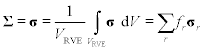 [10.20]
In the case of linear microelastic behaviour of each individual material phase,
σr=ℂr:εr [10.21]
with the fourth-order elasticity tensor ![]() r and ‘:’ indicating second-order tensor contraction, and εr denoting the equilibrated microstrains, the superposition principle implies the existence of concentration tensors Ar
r and ‘:’ indicating second-order tensor contraction, and εr denoting the equilibrated microstrains, the superposition principle implies the existence of concentration tensors Ar![]() linking multilinearly the macrostrains to the average microstrains in phase r:
linking multilinearly the macrostrains to the average microstrains in phase r:
εr=Ar:E [10.22]
Insertion of Eq. [10.21] into Eq. [10.20] and averaging over all phases according to Eq. [10.22] leads to
Σ=∑rfrℂr:Ar:E [10.23]
Introducing the format of macroscopic elasticity as
Σ=ℂ:E [10.24]
Eq. [10.23] readily yields the overall homogenized stiffness ![]() of the RVE as
of the RVE as
ℂ=∑rfrℂr:Ar [10.25]
The concentration tensors Ar![]() can be suitably estimated from matrix-inclusion problem (Eshelby, 1957), according to Zaoui, (2002) and Benveniste (1987), but the corresponding details are application-specific; and we will review models for porous hydroxyapatite polycrystals as well as polymer biomaterials in the following.
can be suitably estimated from matrix-inclusion problem (Eshelby, 1957), according to Zaoui, (2002) and Benveniste (1987), but the corresponding details are application-specific; and we will review models for porous hydroxyapatite polycrystals as well as polymer biomaterials in the following.
10.3.2 Application of composition-to-elasticity conversion technique to ceramic biomaterials
Based on the work of Fritsch et al., (2006, 2009, 2010, 2013), we consider here hydroxyapatite biomaterials as illustrated in Fig. 10.1(b). The latter are represented by one spherical pore phase with zero stiffness and a volume fraction being equal to the nanoporosity, and infinitely many non-spherical crystal solid phases (here needle-shaped, see Fig. 10.7), which are oriented in all space directions, see Fig. 10.8 for an RVE of porous polycrystal. For this micromechanical representation, lying halfway between the traditional micromechanics models of the 1960s with only a few (typically two) phases (Hill, 1965), and very CPU consuming finite element models of polycrystals emerging in more recent years (Meille and Garboczi, 2001), the mathematical format of stress and strain average rules needs to be slightly modified, the latter reading exemplarily as,
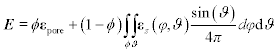
E=ϕεpore+(1−ϕ)∫ϕ∫ϑεs(φ,ϑ)sin(ϑ)4πdφdϑ [10.26]
 [10.26]
with εpore as the average strains found in the pore phase, and with orientation-specific strains εs(φ, ϑ) in the solid crystal phases. Thereby, each orientation in space, quantified through Euler angles φ and ϑ (see Fig. 10.7), is assigned a point on the unit sphere with surface (4π), so that the integral in Eq. [10.26] needs to be normalized by 1/(4π), as to guarantee that the solid phases indeed make up 100 × (1 − ϕ) per cent of the volume of the RVE. Consistently with Eq. [10.26], the concentration relation in the solid phases becomes orientation-dependent,
εS(φ,ϑ)=AS(φ,ϑ):E [10.27]


and the homogenized stiffness reads as
ℂhom=(1−ϕ)ℂHA:∫φ∫ϑAS(φ,ϑ)sin(ϑ)4πdφdϑ [10.28]
 [10.28]
where we restrict ourselves to an isotropic (orientation-independent) stiffness of hydroxyapatite, as the influence of hydroxyapatite anisotropy for homogenized stiffnesses of RVEs such as the one depicted in Fig. 10.8 has been shown to be negligible (Fritsch et al., 2006). Experiments of Katz and Ukraincik (1971) revealed the hydroxyapatite stiffness in terms of bulk moduli and shear moduli as k = 82.60 GPa and G = 44.90 GPa, respectively.
For estimation of the orientation-dependent concentration tensors, we consider each phase (the infinitely many solid ones, and the pore phase) as acting as an inclusion in an infinite matrix with the (so far unknown) stiffness of the homogenized porous polycrystal, subjected to (homogeneous) fictitious strains E∞ at the infinite boundary. The relation between the inclusion strains and fictitious strains were given in Eshelby (1957), as
εs(φ,ϑ)=A∞s(φ,ϑ):E∞εpore(φ,ϑ)=A∞pore(φ,ϑ):E∞A∞s(φ,ϑ)=[I+ℙhomcy1(φ,ϑ):(ℂs−ℂhom)]−1A∞por=[I+ℙhomsph(φ,ϑ):(−ℂhom)]−1 [10.29]
 [10.29]
with ![]() homcyl and
homcyl and ![]() homsph as fourth-order Hill tensors for cylindrical and spherical inclusions, respectively, embedded into a matrix with stiffness
homsph as fourth-order Hill tensors for cylindrical and spherical inclusions, respectively, embedded into a matrix with stiffness ![]() hom The perfect disorder of the crystals in the RVE of Fig. 10.8 and the perfect symmetry of the spherical pores render
hom The perfect disorder of the crystals in the RVE of Fig. 10.8 and the perfect symmetry of the spherical pores render ![]() hom is isotropic, so that it can be given in terms of a bulk modulus khom=Ivol:ℂhom
hom is isotropic, so that it can be given in terms of a bulk modulus khom=Ivol:ℂhom![]() , and a shear modulus Ghom=Idev:ℂhom
, and a shear modulus Ghom=Idev:ℂhom![]() Thereby, Ivol
Thereby, Ivol![]() with components Ivolijkl=1/3δijδkl
with components Ivolijkl=1/3δijδkl![]() is the volumetric part of the unity tensor I
is the volumetric part of the unity tensor I![]() with components Iijkl = 1/2(δikδjl + δilδjk), and Idev=I−Ivol
with components Iijkl = 1/2(δikδjl + δilδjk), and Idev=I−Ivol![]() is the deviatoric part of I
is the deviatoric part of I![]() . The Kronecker delta δij is defined as δij = 0 for i ≠ j and δij = 1 for i = j. The Hill tensors are related to Eshelby tensors via Seshr=ℙhomr:ℂhom
. The Kronecker delta δij is defined as δij = 0 for i ≠ j and δij = 1 for i = j. The Hill tensors are related to Eshelby tensors via Seshr=ℙhomr:ℂhom![]() .The Eshelby tensor Seshsph
.The Eshelby tensor Seshsph![]() corresponding to spherical inclusions (pores in Fig 10.8) reads as
corresponding to spherical inclusions (pores in Fig 10.8) reads as
Seshsph=3khom3khom+4GhomIvol+6(khom+2Ghom)5(3khom+4Ghom)Idev [10.30]
 [10.30]
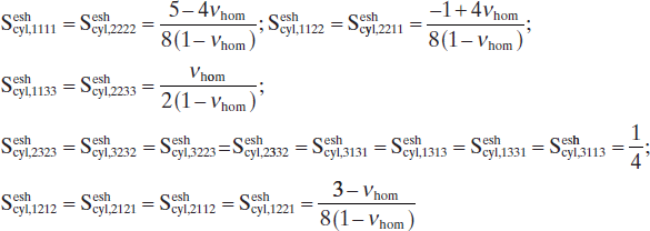
In the base frame (eϑ, eφ, er) (1 = ϑ, 2 = φ, 3 = r, see Fig. 10.8 for Euler angles φ and ϑ), attached to individual solid needles, the non-zero components of the Eshelby tensor Seshcyl![]() corresponding to cylindrical inclusions read as
corresponding to cylindrical inclusions read as
Sesheyl,1111=Sesheyl,2222=5−4νhom8(1−νhom);Seshcyl,1122=Seshsyl,2211=−1+4νhom8(1−νhom);Seshcyl,1133=Seshcyl,2233=νhom2(1−νhom);Seshcyl,2323=Seshcyl,3232=Seshcyl,3223=Seshcyl,2332=Seshcyl,3131=Seshcyl,1313=Seshcyl,1331=Seshcyl,3113=14;Seshcyl,1212=Seshcyl,2121=Seshcyl,2112=Seshcyl,1221=3−νhom8(1−νhom) [10.31]
 [10.31]
with νhom as Poisson’s ratio of the homogenized polycrystal,
νhom=3khom−2Ghom6khom+2Ghom [10.32]
Insertion of Eq. [10.29] into strain average rule, Eq. [10.27], yields a relation between the auxiliary (fictitious) strains at the infinite boundary, and the macroscopic strains acting on the RVE – re-insertion of this relation into Eq. [10.29] leads to the orientation-dependent concentration tensors
As(φ,ϑ)=A∞s(φ,ϑ):[(1−ϕ)2π∫φ=0π∫ϑ=0A∞s(φ,ϑ)sinϑdϑdφ4π+ϕA∞pore]−1Apore=A∞pore:[(1−ϕ)2π∫φ=0π∫ϑ=0A∞s(φ,ϑ)sinϑdϑdφ4π+ϕA∞pore]−1 [10.33]
 [10.33]
Finally, insertion of Eq. [10.30] into Eq. [10.28] yields the homogenized stiffness as
ℂhom=(1−ϕ)ℂHA:〈[I+ℙhomcyl:(ℂHA−ℂhom]−1〉:{(1−ϕ)〈[I+ℙhomcyl(ℂHA−ℂhom)]−1〉+ϕ(I−ℙhomspy:ℂhom)−1}−1 [10.34]
 [10.34]
with the angular average
〈[I+ℙhomcyl:(ℂHA−ℂhom)]−1〉=2π∫φ=0π∫ϑ=0[I+ℙhomcyl(ϑ,φ):(ℂHA−ℂhom)]−1sinϑdϑdφ4π [10.35]
 [10.35]
Following standard tensor calculus (Salençon, 2001), the tensor components of ℙhomcyl(φ,ϑ)=Seshcyl(φ,ϑ)![]() , being related to differently oriented inclusions, are transformed into one, single base frame (e1,e2,e3), in order to evaluate the integrals in Eq. [10.34] and Eq. [10.35].
, being related to differently oriented inclusions, are transformed into one, single base frame (e1,e2,e3), in order to evaluate the integrals in Eq. [10.34] and Eq. [10.35].
The porosity elasticity relation [10.34] and [10.35] has been carefully validated experimentally, see Figs 10.9 and 10.10, for further details refer to Fritsch et al. (2009). We note in passing that such micromechanical representations have been successful also beyond the borders of biomaterial modelling; they are suitable to cover the behaviour of gypsum, piezoelectric ceramics, zirconia, alumina and silicon as well (Sanahuja et al., 2010; Fritsch et al., 2013).


When combining ℂhom Eq. [10.34], with Eq. [10.8], then we arrive at attenuation-elasticity relations as depicted in Figs 10.11 and 10.12. In addition to elastic properties which are heterogeneously distributed across the biomaterial globule, we are also interested in ‘average’ homogeneous solid properties where all solid voxels exhibit the mean nanoporosity averaged over all solid voxels GV > GVthr, amounting ˉϕnano=0.445![]() the corresponding Young’s modulus and Poisson’s ratio of amount to E(ˉϕnano)=23.8GPa
the corresponding Young’s modulus and Poisson’s ratio of amount to E(ˉϕnano)=23.8GPa![]() and ν(ˉϕnano)=0.23
and ν(ˉϕnano)=0.23![]() , respectively.
, respectively.


10.3.3 Application of composition-to-elasticity conversion technique to polymeric biomaterials
Given the matrix-inclusion-type morphology of the microstructure found within the individual voxels of the polymeric material described in Section 10.2.3, we employ the Mori–Tanaka-type scheme (Eshelby, 1957; Mori and Tanaka, 1973; Benveniste, 1987) for determination of the voxel-specific fourth-order (homogenized) stiffness tensor ![]() hom of the PLLA-TCP composite. Therefore, we specify Eq. [10.25] for two material phases, a matrix phase made of PLLA and an inclusion phase made of PLLA;
hom of the PLLA-TCP composite. Therefore, we specify Eq. [10.25] for two material phases, a matrix phase made of PLLA and an inclusion phase made of PLLA;
ℂhom=fTCPATCPℂTCP+(1−fTCP)APLLAℂPLLA [10.36]
In order to estimate the concentration tensor of the TCP inclusion, we compute the homogeneous strains occurring in a spherical inclusion embedded into an infinite fictitious matrix made up of PLLA and subjected to fictitious strains E∞ at the matrix’s infinite boundary; according to Eshelby (1957) they read as
εTCP=[I+ℙPLLA,sph:ℂTCP−ℂPLLA]:E∞ [10.37]
![]() PLLA,sph denotes the fourth-order Hill tensor accounting for the spherical shape of the TCP inclusions embedded in the PLLA-matrix. It is related to Eshelby tensor (Eq. [10.30] with corresponding elastic engineering constants kPLLA and GPLLA) via Seshsph=ℙPLLA,sph:ℂhom
PLLA,sph denotes the fourth-order Hill tensor accounting for the spherical shape of the TCP inclusions embedded in the PLLA-matrix. It is related to Eshelby tensor (Eq. [10.30] with corresponding elastic engineering constants kPLLA and GPLLA) via Seshsph=ℙPLLA,sph:ℂhom![]() . As regards the strains in the PLLA-matrix, replacement, in Eq. [10.37], of εTCP and
. As regards the strains in the PLLA-matrix, replacement, in Eq. [10.37], of εTCP and ![]() TCP by εPLLA and
TCP by εPLLA and ![]() PLLA yields
PLLA yields
εPLLA=E∞ [10.38]
Insertion of Eq. [10.37] and Eq. [10.38] into the strain average rule Eq. [10.18] specified for r = TCP, PLLA, yields a relation between the fictitious matrix strains and the macroscopic strains acting on the RVE, and back-insertion of the latter relation into Eq. [10.37] and Eq. [10.38] yields expression for the concentrations tensors for the TCP and PLLA phases, respectively, Insertion of these concentration expressions into Eq. [10.36] finally yields the homogenized stiffness of the PLLA-TCP composite,
ℂhom={(1−fTCP)ℂPLLA+fTCPℂTCP:[I+ℙPLLA,sph:(ℂTCP−ℂPLLA)]−1}:{(1−fTCP)I+fTCP[I+ℙPLLA,sph:(ℂTCP−ℂPLLA)]−1}−1 [10.39]
 [10.39]
with
ℂPLLA=3kPLLAIvol+2GPLLAIdev [10.40]
and
ℂTCP=3kTCPIvol+2GTCPIdev [10.41]
as the isotropic phase stiffnesses of the matrix and the inclusions, respectively. In Eq. [10.40] and Eq. [10.41] Ivol![]() and Idev
and Idev![]() are respectively the deviatoric and volumetric parts part of the fourth order unity tensor, as defined in Section 10.3.2. Given the strong chemical similarity of TCP and hydroxyapatite (Dorozhkin, 2009), the elastic properties of the latter were considered (see Section 10.3.2). The elastic properties of PLLA, expressed in terms of bulk modulus
are respectively the deviatoric and volumetric parts part of the fourth order unity tensor, as defined in Section 10.3.2. Given the strong chemical similarity of TCP and hydroxyapatite (Dorozhkin, 2009), the elastic properties of the latter were considered (see Section 10.3.2). The elastic properties of PLLA, expressed in terms of bulk modulus
kPLLA=EPLLA/(3(1−2νPLLA)) [10.42]
and of shear modulus
GPLLA=EPLLA/(2(1+2νPLLA) [10.43]
followed from conducted nanoindentation tests, EPLLA = 3.59 GPa (see Luczynski et al., 2013 for details); and from the literature, νPLLA = 0.45 (Balac et al., 2002).
Finally, feeding the homogenized stiffness Eq. [10.39] with the aforementioned elastic properties of PLLA and TCP, as well as with voxel-specific volume fractions derived from attenuation-related grey values according to Eq. [10.16], gives access to grey value-specific Young’s moduli Ehom(GV) and Poisson’s ratios νhom(GV) throughout the scaffold’s solid phase; based on the components of the compliance tensor Dhom=(ℂhom)−1![]() according to:
according to:
Ehom(GV)=1/Dhom1111(GV) [10.44]
νhom(GV)=−Ehom(GV)/Dhom1122(GV) [10.45]
In addition to the respective heterogeneous (grey value-specific) elastic properties throughout the solid portion of the scaffold, we consider also ‘averaged’ homogeneous elastic properties (see Table 10.1). Therefore, we remember that averaging over elastic properties does not per se have a theoretical basis (Zaoui, 2002), while the evaluation of volume fractions within reasonably chosen RVEs is one of the fundamentals of micromechanics. Accordingly, we average over all volume fraction-related grey values in the solid compartment of the microCT image, thus arriving at an averaged grey value GVavg according to
GVavg=1NsolGV=255∑GV=66(NGV×GV)=90 [10.46]
with Nsol as the total number of voxels in the solid portion of the scaffold, and NGV as the number of voxels with grey value GV. Specification of Eq. [10.44] and Eq. [10.45] for GV = GVavg yields the ‘average’ homogeneous elastic properties in terms of Young’s modulus and Poisson’s ratio as EGVavg = 4.51 GPa and νGVavg = 0.44, respectively (see also Table 10.1).
Table 10.1
Elastic properties related to solid compartment of scaffold: poly-L-lactide (PLLA) from nanoindentation and micromechanics, tri-calcium phosphate (TCP) from ultrasonic experiments, ‘average’ PLLA-TCP nanocomposite from micromechanics
| Young’s modulus [GPa] | Poisson’s ratio | |
| PLLA | 3.59 | 0.45 |
| TCP | 114.04 | 0.27 |
| PLLA-TCP | 4.52 | 0.44 |
10.4 Intravoxel-micromechanics-enhanced finite element simulations
10.4.1 Voxel-to-element conversion technique
The voxel-specific elastic properties obtained in Section 10.3 are finally used for feeding finite element models with validated, reliable material properties. Therefore, different amounts of neighbouring voxels are merged into finite elements. The different merging options are quantified through merging factors, being identical to the third power of the number of voxels defining the length of one edge of the finite element cubes. As regards the ceramic biomaterial globule, we considered merging factors of 40 × 40 × 40 = 64 000 voxels, 30 × 30 × 30 = 27 000 voxels, 20 × 20 × 20 = 8000 voxels, 15 × 15 × 15 = 3375 voxels, 12 × 12 × 12 = 1728 voxels, 10 × 10 × 10 = 1000 voxels, 9 × 9 × 9 = 729 voxels, 8 × 8 × 8 = 512 voxels, 7 × 7 × 7 = 343 voxels, 5 × 5 × 5 = 125 voxels, and 4 × 4 × 4 = 64 voxels; corresponding finite element models consisted of 0.9 × 10³, 2.4 × 10³, 8.5 × 10³, 20.7 × 10³, 41.1 × 10³, 71.9 × 10³, 99.2 × 10³, 142.1 × 10³, 213.8 × 10³, 595.1 × 10³, 1171.2 × 103 finite elements, As regards the polymer biomaterial scaffold, we considered merging factors of 8 × 8 × 8, 7 × 7 × 7, 6 × 6 × 6, 5 × 5 × 5 and 4 × 4 × 4 voxels; corresponding finite element models consisted of 1.1 × 10⁵, 1.7 × 10⁵, 2.7 × 10⁵, 4.8 × 10⁵ and 9.6 × 10⁵ finite elements. All these finite elements are assigned the grey-scaled attenuation values averaged over all the voxels which were merged into the considered finite element. However, if the assigned grey values turned out to be smaller than the threshold values given in Sections 10.2.2 and 10.2.3, GVthr = 139 in the case of the hydroxyapatite globule, and GVthr = 65 in the case of the polymer biomaterial scaffold; then the corresponding finite elements were skipped; otherwise, they were assigned nanoporosities according to Eq. [10.7] in the case of porous hydroxyapatite, and TCP volume fractions according to Eq. [10.16] in the case of the TCP-reinforced PLLA matrix. Then, we apply application-specific boundary conditions to the described ceramic and polymer biomaterials, before typical simulation results are presented, again in biomaterial-specific sections.
10.4.2 Behaviour of ceramic biomaterial globules
The hydroxyapatite globules are typically compiled into a large bone defect, so that they constitute some ‘granular material’. Hence, the loading of each granule is governed by globule-to-globule contact. As to mimic this mechanical situation while only considering a single granule, we here consider ‘uniaxial’ compression of this single globule, in the form of slightly distributed forces on both ‘poles’ of the globule. This is realized in terms of prescribed displacements in the loading direction, amounting to zero at plane ‘BC3’ in Fig. 10.13, and to 0.1% of the globule diameter, at plane ‘BC1’ in the same figure. In the ‘BC1’-plane, boundary condition ‘BC2’ indicates fixed displacements perpendicular to the loading direction. The magnitude of the prescribed displacements is chosen as to mimic normal physiological strain states, which are typically in the order of 1000 microstrains (Viceconti and Seireg, 1990; Taylor, 1998; Hsieh et al., 2001).

Applying these boundary conditions to all the finite element meshes reported in Section 10.4.1 yields a convergence study (see Fig. 10.14), which shows that 600 000 finite elements are needed in order to achieve a discretization-dependent precision of about 10%. Hence, we now focus in the results from the finite element model consisting of 1 171 176 finite elements (3 965 253 degrees of freedom). The forces needed to compress the heterogeneous granule are by 5% smaller than those needed to compress a globule with homogeneous solid properties derived from the mean nanoporosity in all solid finite elements (Table 10.2). Hence, neglection of the heterogeneity in the solid leads to some overestimation of the global stiffness of the investigated granule. This difference in global stiffness is consistent with the first-order moment of deviatoric stresses in the (solid) finite elements, computed according to Dormieux et al. (2002)
ˉσdev=√12〈σdev(x)〉:〈σdev(x)〉 [10.47]
with
〈(.)〉=1VS∫VS(.)dV [10.48]
 [10.48]
as the average of quantity (.) over all (solid) finite elements, filling volume Vs. In Eq. (10.45), the deviatoric stresses σdev(x) are defined as
σdev(x)=σ(x)−131tr[σ(x)] [10.49]
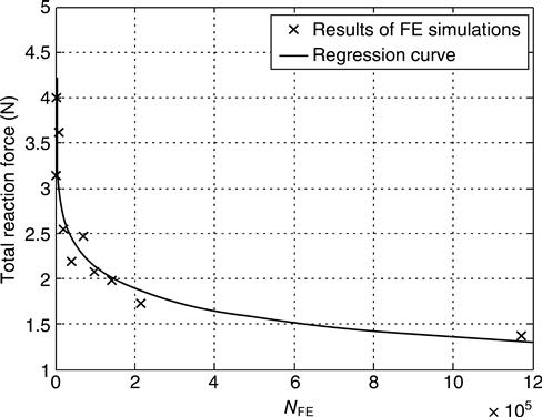
Table 10.2
Reaction forces at the poles of the granule, for homogeneous and heterogeneous (element-specific) elastic properties
| Component | Heterogeneous value (N) | Homogeneous value (N) |
| Rz | 1.386 | 1.454 |
In fact, the first-order moment of deviatoric stresses is larger in the homogeneous than in the heterogeneous simulations (see Table 10.3). On the other hand, the variability of different stress states throughout the solid finite elements is larger in the heterogeneous analysis, when compared to the homogeneous analysis, which can be seen from the second-order moments of deviatoric stresses, defined as
ˉˉσdev=√12〈σdev(x)〉=√12〈σdev(x):σdev(x)〉 [10.50]
Table 10.3
First- and second-order moments of deviatoric stresses, for homogeneous and heterogeneous (element-specific) elastic properties
| Moment | Heterogeneous value (Pa) | Homogeneous value (Pa) |
| ˉσdev |
5.25 × 10⁵ | 5.48 × 10⁵ |
| ˉˉσdev |
2.56E6 × 106 | 2.48 × 10⁶ |

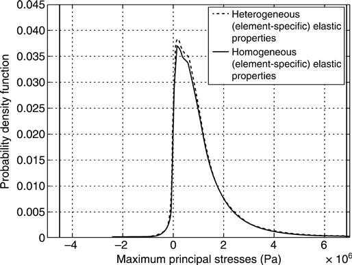
This stress variability differences can be also seen from the histogram of the deviatoric stress norms (Fig. 10.15) and of the maximum principal stress (largest eigenvalue of stress tensor, see Fig. 10.16). Distribution plots of deviatoric stress norms and maximum principal stresses throughout the considered structure (Figs 10.17 and 10.18) reveal that stress peaks occur at the load introduction areas, and around crack-like structures, rather than close to the walls of pseudo-spherically shaped micropores. This suggests that the microcracks are the key microstructural features governing the stiffness of the overall globule. In order to further quantify this important function of the cracks, the results of the aforementioned simulations are compared to the analytical solution for spheres compressed at their poles, whereby the material building up the spheres consists of a matrix with elastic properties corresponding to the mean nanoporosity of ˉϕnano=0.445![]() , with spherical micropores (but no cracks) being embedded into the aforementioned matrix (these micropores filling a microporosity of Φmicro = 0.189). The elastic properties of such a material are determined by the well-known Mori–Tanaka method (Mori and Tanaka, 1973; Benveniste, 1987), and its shear modulus, amounting to G = 6.45 GPa, enters the analytical formula of Lurje for a homogeneous sphere subjected to forces at its poles (Lurje, 1963):
, with spherical micropores (but no cracks) being embedded into the aforementioned matrix (these micropores filling a microporosity of Φmicro = 0.189). The elastic properties of such a material are determined by the well-known Mori–Tanaka method (Mori and Tanaka, 1973; Benveniste, 1987), and its shear modulus, amounting to G = 6.45 GPa, enters the analytical formula of Lurje for a homogeneous sphere subjected to forces at its poles (Lurje, 1963):
Z=Δr·G·r0−0.127 [10.51]
where Z gives the (compressive) force at the poles of the sphere (reaction force). This force is compared to the results of the finite element simulations. Δr denotes the change in radius that was applied as boundary condition ‘BC1’ (Fig. 10.13), and r0 is the original granule radius. A corresponding reaction force of Z = 112 N (estimated from Eq. 10.51), being approximately 80 times larger than those from heterogeneous and homogeneous finite element analyses (see convergent forces in Fig. 10.14), clearly identifies the crack-like features in the investigated globule as the by far dominant stiffness-governing feature.


10.4.3 Behaviour of polymer biomaterial scaffolds
The finite element models described in Section 10.4.1 are subjected to uniaxial compression conditions in vertical (longitudinal) direction (orthogonal to the rapid-prototyped ‘beams’, ‘piled’ on each other), indicated by (vertical) unit vector e3 in Figs 10.19 and 10.20. While the bottom surface of the meshed construct is held at fixed displacements in e3 direction (and free to move in all other directions), a vertical displacement amounting to 5% of the scanned object height is prescribed at the top surface. The lateral walls of the scaffold are kept stress-free. Evaluation of results comprises the following steps: all reaction forces in e3 direction triggered at the nodes of the upper surface of the finite element mesh are summed up to one reaction force F, which is then used for evaluation of a macroscopic, whole scaffold-related, Young’s modulus (EFE) as follows
EFE=Fl3A·Δl3 [10.52]
with A as the area of the loaded surface, and Δl3 / l3 = 0.05; see Fig. 10.21, for the results obtained from all meshes described in Section 10.4.1.


From Fig. 10.21, it becomes obvious that all meshes deliver, numerically speaking, fully converged results. Moreover, the overall deformation under macroscopic uniaxial load is fairly independent on the actual microscopic distribution of elastic properties, as follows from the fair agreement of the results obtained from simulations based on heterogeneous and homogeneous material properties, respectively (see Table 10.4).
Table 10.4
Finite element-predicted macroscopic scaffold-related Young’s modulus averaged over the values given in Fig. 10.21 for homogeneous and heterogeneous microscopic elastic properties
| < EFE > [MPa] | |
| Heterogeneous model | 145.02 ± 1.68 |
| Homogenous model | 140.71 ± 1.28 |
| Averaged over both models | 142.86 ± 2.68 |
We may still question the physical representation of the scaffold, i.e. the appropriateness of the assignment of the (element-specific or overall averaged) elastic properties. In order to check the latter, we compare the macroscopic elastic modulus derived from the finite element simulations with direct measurements of this property. The latter stemmed from the unloading portion of the load–displacement curve in uniaxial mechanical experiments performed by means of an electromechanical testing stand as described in Luczynski et al. (2012, 2013). These tests resulted in an experimental macroscopic Young’s modulus of the scaffold amounting to Eunl = 125.5 ± 19.33 MPa (mean value ± standard deviation).
This value perfectly confirms the relevance of our simulated value of EFE = 142.86 ± 2.68 MPa (mean value ± standard deviation evaluated over all simulations recorded in Fig. 10.21, see also Table 10.4). This supports our confidence into the chosen modelling approach, which motivates us to also evaluate the scaffold’s transverse Poisson’s ratios ν31 and ν32 from the FE simulations described above; according to the following procedure (Luczynski et al., 2012): the macroscopic scaffold strains are determined from the displacements averaged over the six scaffold surfaces
Eii=(u+i−u−i)/li;fori=1,2,3 [10.53]
with li as the lineal dimensions of the overall scaffold (in directions i = 1, 2, 3), u+i as the average displacement of the three scaffold walls with normals pointing in directions ei, and ui−![]() as the average displacements of the three scaffold walls pointing in the opposite direction – ei. From these normal strains, the Poisson’s ratios follow as
as the average displacements of the three scaffold walls pointing in the opposite direction – ei. From these normal strains, the Poisson’s ratios follow as
ν31=−E11/E33 [10.54]
ν32=−E22/E33 [10.55]
given in Fig. 10.22 and Table 10.5. Similar to the situation encountered with the longitudinal macroscopic Young’s modulus, they do not vary too much between the simulations with heterogeneous and homogeneous material properties. Furthermore, the rather small difference between ν32 and ν31 suggests that the scaffold might be regarded as roughly cubic at the macroscale. A corresponding quasi-cubic Poisson’s ratio averaged over all values depicted in Fig. 10.22, amounts to 0.0638 ± 0.0136.

Table 10.5
Transverse Poisson’s ratios of the macroscopic scaffold computed from FE simulations, based on a mesh with 1.1 × 10⁵ number of elements
| ν31 | ν32 | |
| Heterogeneous model | 0.0593 ± 0.0024 | 0.0596 ± 0.0045 |
| Homogenous model | 0.0586 ± 0.0038 | 0.0779 ± 0.0224 |
| Averaged over both models | 0.0590 ± 0.0030 | 0.0687 ± 0.0180 |
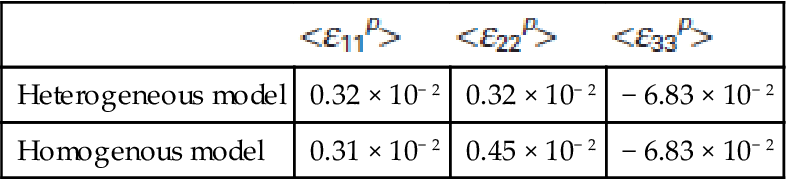
We note that the macroscopic Poisson’s ratio is significantly lower than that of the PLLA-TCP composite solid (amounting to 0.44, see Table 10.1). This indicates that on the microstructural level, the solid phase undergoes much less deformation and strain than the pore phase. In order to quantify this effect, we apply the strain average rule of micromechanics, Eq. [10.18] to the entire scaffold. It allows us to derive from the average microstrain components in the solid phase εijs,i,j=1,2,3![]() , obtained directly from the simulations, the average strains εijp,i,j=1,2,3
, obtained directly from the simulations, the average strains εijp,i,j=1,2,3![]() in the pores, according to
in the pores, according to
εpij=[Eij−(1−Φ)εsij]/Φ;fori,j=1,2,3 [10.56]
where Φ stands for the macroporosity of the scaffold, as given in Section 10.2.3. Indeed, the average vertical normal strains in the pores are much larger than those in the solid (compare ε33s![]() s and ε33p
s and ε33p![]() in Table 10.6 and Table 10.7). This is consistent with the very localized (‘concentrated’) stress and strain peaks in the solid, occurring only at the joints between the individual ‘struts’ ‘piled’ one above the other, see Fig. 10.23 and Fig. 10.24 for principal strain and stress distributions across the investigated structure. The shear microstrains, both in the solid and in the pores, are at least two orders of magnitude smaller than the normal microstrains, which indicates that the overall scaffold’s deformation process is largely ‘free’ from shear deformations.
in Table 10.6 and Table 10.7). This is consistent with the very localized (‘concentrated’) stress and strain peaks in the solid, occurring only at the joints between the individual ‘struts’ ‘piled’ one above the other, see Fig. 10.23 and Fig. 10.24 for principal strain and stress distributions across the investigated structure. The shear microstrains, both in the solid and in the pores, are at least two orders of magnitude smaller than the normal microstrains, which indicates that the overall scaffold’s deformation process is largely ‘free’ from shear deformations.
Table 10.6
Microstrains averaged over solid compartment of scaffold < εs>, for heterogeneous and homogeneous simulations with 1.1 × 10⁵ elements; index ‘3’ labels (longitudinal) loading direction, indices ‘1’ and ‘2’ label (transverse) orthogonal to the loading directions
| <ε11s> |
<ε22s> |
<ε33s> | |
| Heterogeneous model | (0.24 ± 0.00) × 10− 2 | (0.24 ± 0.00) × 10− 2 | (− 0.54 ± 0.02) × 10− 2 |
| Homogenous model | (0.24 ± 0.00) × 10− 2 | (0.24 ± 0.00) × 10− 2 | (− 0.54 ± 0.02) × 10− 2 |

Table 10.7
Average microstrains in pores < εp>, computed from average microstrains in solid and macro strains according to Eq. 10.56 for heterogeneous and homogeneous simulations with 1.1 × 10⁵ elements; index ‘3’ labels (longitudinal) loading direction, indices ‘1’ and ‘2’ label (transverse) orthogonal to the loading directions
| <ε11p> |
<ε22p> |
<ε33p> | |
| Heterogeneous model | 0.32 × 10− 2 | 0.32 × 10− 2 | − 6.83 × 10− 2 |
| Homogenous model | 0.31 × 10− 2 | 0.45 × 10− 2 | − 6.83 × 10− 2 |


As concerns the influence of micro-heterogeneities, the homogeneous model delivered a marginally lower value of the first order moment of deviatoric stresses, Eq. [10.47], than the heterogeneous one (see Table 10.8). This means that the homogeneous model is slightly softer than the heterogeneous one, which is in agreement with the macroscopic Young’s moduli reported in Table 10.4. Also the second order moment of deviatoric stresses, defined through Eq. [10.50], was (albeit only slightly) higher in the heterogeneous model than in the homogeneous one (see Table 10.8). This indicates a slightly higher heterogeneity of the microstress distribution in the heterogeneous as compared to the homogeneous simulations.
10.5 Conclusions and future trends
In this chapter, we have summarized a novel method for converting X-ray attenuation information into voxel-specific elastic properties, for subsequent use in structural analyses based on the finite element method. As opposed to earlier purely empirical approaches with a limited applicability range, the new method, while combining fundamental laws of X-ray physics with continuum micromechanics of materials, provides reliable mechanical properties. This holds the promise for unprecedented avenues in biomaterials design, i.e. for in-silico dimensioning of scaffolds according to mechanical requirements. In a first stage, this has allowed us to reveal the governing mechanical features in biomaterial scaffolds, as the cracks in the hydroxyapatite globule in Section 10.4.2, or the highly stressed ‘beam-contacts’ in Section 10.4.3. In a second stage, this may enable a real ‘fracture risk assessment’ of biomaterials under extreme conditions. This latter promise for safety prediction becomes the more reality, the more different mechanical properties, also beyond elasticity, can be retrieved from CT images. This proposes the next logical step in the work described here, namely relating CT-derived volume fractions not only to elastic properties, as shown in Section 10.3, but also to strength properties of biomaterials, through respective micromechanics models (Fritsch et al., 2009, 2010, 2013). At the same time, our combined X-ray physics-continuum micromechanics method can be also applied to microCT images of biological tissues such as bone, as was recently reported in Blanchard et al. (2013). This proposes another thread of future research, related to evaluation of tissue engineering construct with tissue engineered bone growing within them, as scanned by Mastrogiacomo et al., (2004, 2005) with again two stages: (i) fundamental characteristics of load-carrying behaviour and (ii) fracture risk evolution during tissue regeneration. The latter can be retrieved from a temporal series of scans – or, in a very mature state of in-silico biomaterials design, from systems biology-based modelling of tissue growth, as was recently developed for bone at the micrometre-to-millimetre scale (Scheiner et al., 2013). This all very clearly shows how engineering science-rooted methods may continuously enrich and transform the biomaterials field.
10.6 Acknowledgements
All authors acknowledge financial support through project COST MP1005 NAMABIO, entitled ‘From nano to macro biomaterials (design, processing, characterization, modelling) and applications to stem cells regenerative orthopedic and dental medicine’, sponsored by COST, The European Cooperation in Science and Technology. Krzysztof Luczynski, Alexander Dejaco, and Christian Hellmich additionally acknowledge financial support from project ERC-2010-StG 257023-MICROBONE ‘Multiscale poro-micromechanics of bone materials, with links to biology and medicine’.
10.8 Appendix: nomenclature
A area of the loaded surface in the PLLA-TCP tissue engineering scaffold
APLLA![]() fourth-order strain concentration tensor of PLLA
fourth-order strain concentration tensor of PLLA
Ar![]() fourth-order strain concentration tensor of phase r
fourth-order strain concentration tensor of phase r
ATCP![]() fourth-order strain concentration tensor of TCP
fourth-order strain concentration tensor of TCP
Ahomr![]() homogenized fourth-order strain concentration tensor of phase r
homogenized fourth-order strain concentration tensor of phase r
![]() hom homogenized fourth-order stiffness tensor
hom homogenized fourth-order stiffness tensor
![]() HA fourth-order stiffness tensor of single hydroxyapatite crystals
HA fourth-order stiffness tensor of single hydroxyapatite crystals
![]() PLLA fourth-order stiffness tensor of PLLA
PLLA fourth-order stiffness tensor of PLLA
![]() r fourth-order stiffness tensor of phase r
r fourth-order stiffness tensor of phase r
![]() TCP fourth-order stiffness tensor of TCP
TCP fourth-order stiffness tensor of TCP
d characteristic length of an inhomogeneity within an RVE
Dhom![]() homogenized fourth-order homogenized compliance tensor
homogenized fourth-order homogenized compliance tensor
Ehom homogenized Young’s modulus of PLLA-TCP tissue engineering scaffold
EFE Young’s modulus of PLLA-TCP tissue engineering scaffold derived from finite element model
EPHA isotropic Young’s modulus of nanoporous HA
Eunl Young’s modulus of PLLA-TCP tissue engineering scaffold derived from unloading portion of force–displacement characteristics, stemming from uniaxial compression tests
E second-order ‘macroscopic’ strain tensor
Eii macroscopic strain measured in the ii direction
Eij macroscopic strain measured in the ij direction
E∞ second-order strain tensor corresponding to a fictitious strain applied at the infinite boundary
e1 + e2 + e3 unit base vectors of Cartesian reference base frame
eϑ,eϕ,er unit base vectors of Cartesian local base frame of a single crystal
F reaction forces in the PLLA-TCP tissue engineering scaffold derived from the finite element model
GHA shear modulus of single hydroxyapatite crystals
GV X-ray attenuation-related grey value
GVavg average X-ray attenuation-related grey value
GVair X-ray attenuation-related grey value of air
GVr X-ray attenuation-related grey value of phase r
GVHA X-ray attenuation-related grey value of pure hydroxyapatite
GVPLLA X-ray attenuation-related grey value of pure PLLA
GVTCP X-ray attenuation-related grey value of pure TCP
GVthr threshold X-ray attenuation-related grey value separating air-filled voxels from solid voxels
I![]() fourth-order identity tensor
fourth-order identity tensor
Ivol![]() volumetric part of fourth-order identity tensor I
volumetric part of fourth-order identity tensor I![]()
Idev![]() deviatoric part of fourth-order identity tensor I
deviatoric part of fourth-order identity tensor I![]()
kHA bulk modulus of single hydroxyapatite crystals
l characteristic length of RVE
L characteristic length of a structure containing an RVE
l3 height of the PLLA-TCP tissue engineering scaffold in the loading direction
li length of the PLLA-TCP tissue engineering scaffold in the i direction
ls length of a hydroxyapatite biomaterial sample
N orientation vector aligned with longitudinal axis of needle
Nr number of phases within an RVE
n orientation vector perpendicular to N
Nsol total number of voxels in the solid phase
NGV number of voxels characterized with grey value GV
![]() PLLA,sph fourth-order Hill tensor characterizing the interaction between the spherical TCP inclusions and the matrix
PLLA,sph fourth-order Hill tensor characterizing the interaction between the spherical TCP inclusions and the matrix ![]() PLLA
PLLA
![]() homr fourth-order Hill tensor characterizing the interaction between the phase r and the matrix
homr fourth-order Hill tensor characterizing the interaction between the phase r and the matrix ![]() hom
hom
![]() homcyl fourth-order Hill tensor for cylindrical inclusion in matrix with stiffness
homcyl fourth-order Hill tensor for cylindrical inclusion in matrix with stiffness ![]() hom
hom
![]() homsph fourth-order Hill tensor for spherical inclusion in matrix with stiffness
homsph fourth-order Hill tensor for spherical inclusion in matrix with stiffness ![]() hom
hom
p(GV) probability density function of attenuation-related grey values
RVE representative volume element
Rz reaction forces at the poles of the HA granule
Sesh,0r![]() fourth-order Eshelby tensor for phase r embedded in matrix
fourth-order Eshelby tensor for phase r embedded in matrix ![]() 0
0
Seshcyl![]() fourth-order Eshelby tensor for cylindrical inclusion embedded in isotropic matrix with stiffness
fourth-order Eshelby tensor for cylindrical inclusion embedded in isotropic matrix with stiffness ![]() poly
poly
Seshsph![]() fourth-order Eshelby tensor for spherical inclusion embedded in isotropic matrix with stiffness
fourth-order Eshelby tensor for spherical inclusion embedded in isotropic matrix with stiffness ![]() poly
poly
tr trace of a second-order tensor
Vsolid volume of the solid phase
δij Kronecker delta (components of second-order identity tensor 1)
Δl3 compressive displacement applied to the PLLA-TCP tissue engineering scaffold
εpore second-order strain tensor field of pore phase
εr second-order strain tensor field of phase r
εs second-order strain tensor field of solid phase
εijp![]() average strain in the pores in ij direction
average strain in the pores in ij direction
εijs![]() average strain in the solid in ij direction
average strain in the solid in ij direction
ϑ latitudinal cordinate of spherical coordinate system
μ X-ray attenuation coefficient
μr X-ray attenuation coefficient of phase r
ν31 Poisson’s ratio of the PLLA-TCP tissue engineering scaffold in the direction ‘31’
ν32 Poisson’s ratio of the PLLA-TCP tissue engineering scaffold in the direction ‘32’
νhom homogenized Poisson’s ratio of monoporosity biomaterial made of hydroxyapatite
ν hom homogenized Poisson’s ratio of PLLA-TCP tissue engineering scaffold
ξ displacements within an RVE and at its boundary
ρHA mass density of pure hydroxyapatite
ρvox mass density of a single voxel
Σ second-order ‘macroscopic’ stress tensor
ΣPLLA second-order ‘macroscopic’ stress tensor of PLLA matrix
σdev(x) deviatoric stresses at position x
ˉσdev![]() first-order moment of deviatoric stresses
first-order moment of deviatoric stresses
ˉˉσdev![]() second-order moment of deviatoric stresses
second-order moment of deviatoric stresses
σr second-order stress tensor field of phase r
φ longitudinal coordinate of spherical coordinate system
ϕnano voxel-specific nanoporosity
ϕtotal total (micro and nano) voxel-specific porosity
ψ longitudinal coordinate of vector n
〈(.)〉V = 1/V∫V(.)V average of quantity (.) over volume V