
The data visualization tools in Excel 2007 represent one of its best new features. Microsoft added a new drawing layer that can hold icon sets, data bars, and color scales. Unlike SmartArt graphics, Microsoft exposed the entire object model for the data visualization tools, so you can use VBA to add data visualizations to your reports.
Excel 2007 provides a variety of new data visualizations. A description of each appears below, with an example shown in Figure 15.1 on the next page.
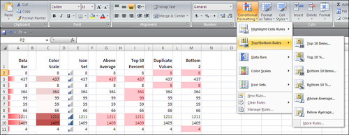
Data bars—. The data bar adds an in-cell bar chart to each cell in a range. The largest numbers have the largest bars, and the smallest numbers have the smallest bars. You can control the bar color as well as the values that should receive the smallest and largest bar.
Color scales—. Excel applies a color to each cell from among a two- or three-color gradient. The two-color gradients are best for reports that will be presented in monochrome. The three-color gradients require a presentation in color, but can represent a report in a traditional traffic light color combination of red-yellow-green. You can control the points along the continuum where each color begins and you can control the two or three colors.
Icon sets—. Excel assigns an icon to each number. Icon sets can contain three icons (such as the red, yellow, green traffic lights), four icons, or five icons (such as the cell phone power bars). With icon sets, you can control the numeric limits for each icon, reverse the order of the icons, or choose to show only the icons.
Above/below average—. Found under the top/bottom rules fly-out menu, these rules make it easy to highlight all of the cells that are above average. You can choose the formatting that should be applied to the cells. Note in column G of Figure 15.1 only 30 percent of the cells are above average. Contrast with the top 50 percent in column I.
Top/bottom rules—. Excel highlights the top or bottom n percent of cells, or highlights the top or bottom n cells in a range.
Duplicate values—. Excel highlights any values that are repeated within a dataset. Because the new Delete Duplicates command on the Data tab of the Ribbon is so destructive, you might prefer to highlight the duplicates and then intelligently decide which records to delete.
Highlight cells—. The legacy conditional formatting rules, such as greater than, less than, between, and text that contains, are still available in Excel 2007. The powerful Formula conditions are also available, although you might have to use these less frequently with the addition of the average and top/bottom rules.
All the data visualization settings are managed in VBA with the FormatConditions collection. Excel 2007 adds seven new methods for adding conditions, such as the AddDataBar, AddIconSet, AddTop10, AddUniqueValues, and so on.
In Excel 2007, it is possible to apply several different conditional formatting conditions to the same range. For example, you can apply a two-color color scale, an icon set, and a data bar to the same range. Excel 2007 adds a Priority property to specify which conditions should be calculated first. Methods such as SetFirstPriority and SetLastPriority ensure that a new format condition is executed before or after all others.
The StopIfTrue property works in conjunction with the Priority property. In the “Using Visualization Tricks” section later in this chapter, you will see how to use the StopIfTrue property on a dummy condition to make other formatting apply only to certain subsets of a range.
The Type property has been dramatically expanded in Excel 2007. Whereas this property formerly was a toggle between CellValue and Expression, 13 new types were added in Excel 2007. Table 15.1 shows the valid values for the Type property. Items 3 through 18 are new in Excel 2007.
Table 15.1. Valid Types for a Format Condition
Value | Description | VBA Constant |
|---|---|---|
1 | Cell value |
|
2 | Expression |
|
3 | Color scale |
|
4 | Data bar |
|
5 | Top 10 values |
|
6 | Icon set |
|
8 | Unique values |
|
9 | Text string |
|
10 | Blanks condition |
|
11 | Time period |
|
12 | Above average condition |
|
13 | No blanks condition |
|
16 | Errors condition |
|
17 | No errors condition |
|
18 | Compare columns |
|
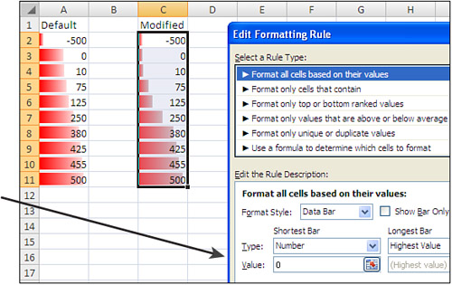
The Data Bar command adds an in-cell bar chart to each cell in a range. Typically, the smallest values in the dataset receive a bar that is 4 pixels wide. The largest values in the dataset receive a bar that is 90 percent of the width of the cell.
In Figure 15.2, a value of -500 in cell A2 causes small values such as 0 and 10 in cells A3:A4 to have a relatively large data bar. By using the Edit Formatting Rule dialog, you can specify that any value of 0 or less should get the smallest data bar. In column C, the size of each data bar better represents the expected values of 0 to 500.
Use the FormatConditions.AddDataBar method to add a new FormatCondition member to the FormatConditions collection for a range:
Range("A1:A10").FormatConditions.AddDatabarBecause you can’t be sure that you have only one condition applied to a range, you should refer to the new data bar condition by using the Count property:
ThisCond = Range("A1:A10").FormatConditions.CountIf you want to make sure that this is the only format condition applied to the range, use the FormatConditions.Delete method:
Rang Range("A1:A10").FormatConditions.DeleteSpecify a color for the data bar using the Color and TintAndShade properties for the BarColor. The Color property can be any of 16 million colors. Define it using the RGB function. The TintAndShade property will modify the selected color. Specify a value from -1 (darkest) to 1 (lightest). The following code changes the color of the data bar to red and makes it darker than usual:
With Range("A1:A10").FormatConditions(ThisCond).BarColor
    .Color = RGB(255, 0, 0) ' Red
    .TintAndShade = -0.5 ' Darker than normal
End With
By default, Excel assigns the shortest data bar to the minimum value and the longest data bar to the maximum value. If you want to override the defaults, use the Modify method for either the MinPoint or MaxPoint properties. Specify a type from those shown in Table 15.2. Types 0, 3, 4, and 5 require a value. Table 15.2 shows valid types.
Table 15.2. MinPoint and MaxPoint Types
Description | VBA Constant | |
|---|---|---|
| Number is used. |
|
| Lowest value from the list of values. |
|
| Highest value from the list of values. |
|
| Percentage is used. |
|
| Formula is used. |
|
| Percentile is used. |
|
| No conditional value. |
|
To have the smallest bar assigned to values of 0 and below, use this code:
Range("A1:A10").FormatConditions(ThisCond).MinPoint.Modify _
    Newtype:=xlConditionValueNumber, NewValue:=0
To have the top 20 percent of the bars have the largest bar, use this code:
Range("A1:A10").FormatConditions(ThisCond).MaxPoint.Modify _
    Newtype:=xlConditionValuePercent, NewValue:=80
An interesting alternative is to only show the data bars and not the value. To do this, use this code:
Range("A1:A10").FormatConditions(ThisCond).ShowValue = FalseTo create the data bars shown in column C of Figure 15.2, use this code:
Sub AddDataBar()
' Add a Data bar
' Ensure any credits < 0 have a data bar like 0
'
    With Range("A1:A10")
        ' Add the data bars
        .FormatConditions.AddDataBar
        ' Set the lower limit
        ThisCond = .FormatConditions.Count
        .FormatConditions(ThisCond).MinPoint.Modify _
            newtype:=xlConditionValueNumber, newvalue:=0
        ' Use red, darker than usual
        With .FormatConditions(ThisCond).BarColor
            .Color = RGB(255, 0, 0)
            .TintAndShade = -0.5
        End With
    End With
End SubColor scales can be added in either two-color or three-color scale varieties. Figure 15.3 shows the available settings in the Excel user interface for a color scale using three colors.
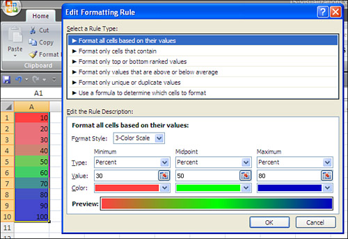
Like the data bar, a color scale is applied to a range object using the AddColorScale method. You should specify a ColorScaleType of either 2 or 3 as the only argument of the AddColorScale method.
You then indicate a color and tint for either both, or all three of the color scale criteria. You can also specify if the shade is applied to the lowest value, highest value, a particular value, a percentage, or at a percentile using the values shown previously in Table 15.2.
The following code generates a three-color color scale in range A1:A10:
Sub Add3ColorScale()
    With Range("A1:A10")
        .FormatConditions.Delete
        ' Add the Color Scale as a 3-color scale
        .FormatConditions.AddColorScale ColorScaleType:=3

        ' Format the first color as light red
        .FormatConditions(1).ColorScaleCriteria(1).Type = xlConditionValuePercent
        .FormatConditions(1).ColorScaleCriteria(1).Value = 30
        .FormatConditions(1).ColorScaleCriteria(1).FormatColor.Color = _
            RGB(255, 0, 0)
        .FormatConditions(1).ColorScaleCriteria(1).FormatColor.TintAndShade = 0.25

        ' Format the second color as green at 50%
        .FormatConditions(1).ColorScaleCriteria(2).Type = xlConditionValuePercent
        .FormatConditions(1).ColorScaleCriteria(2).Value = 50
        .FormatConditions(1).ColorScaleCriteria(2).FormatColor.Color = _
            RGB(0, 255, 0)
        .FormatConditions(1).ColorScaleCriteria(2).FormatColor.TintAndShade = 0

        ' Format the third color as dark blue
        .FormatConditions(1).ColorScaleCriteria(3).Type = xlConditionValuePercent
        .FormatConditions(1).ColorScaleCriteria(3).Value = 80
        .FormatConditions(1).ColorScaleCriteria(3).FormatColor.Color = _
            RGB(0, 0, 255)
        .FormatConditions(1).ColorScaleCriteria(3).FormatColor _
            .TintAndShade = -0.25
    End With

End SubIcon sets in Excel come with three, four, or five different icons in the set. Figure 15.4 shows the settings for an icon set with five different icons.
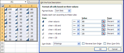
To add an icon set to a range, use the AddIconSet method. No arguments are required. You can then adjust three properties that apply to the icon set. You then use several additional lines of code to specify the icon set in use and the limits for each icon.
After adding the icon set, you can control whether the icon order is reversed, whether Excel shows only the icons, and then specify 1 of the 16 built-in icon sets:
With Range("A1:C10")
    .FormatConditions.Delete
    .FormatConditions.AddIconSetCondition
    ' Global settings for the icon set
     With .FormatConditions(1)
        .ReverseOrder = False
        .ShowIconOnly = False
        .IconSet = ActiveWorkbook.IconSets(xl5CRV)
    End With
End With
Note
It is somewhat curious that the IconSets collection is a property of the active workbook. This seems to indicate that in future versions of Excel, new icon sets might be available.
Table 15.3 shows the complete list of icon sets.
Table 15.3. Available Icon Sets and Their VBA Constants
Icon | Value | Description | Constant |
|---|---|---|---|
| 1 | 3 arrows |
|
| 2 | 3 arrows gray |
|
| 3 | 3 flags |
|
| 4 | 3 traffic lights 1 |
|
| 5 | 3 traffic lights 2 |
|
| 6 | 3 signs |
|
| 7 | 3 symbols |
|
| 8 | 3 symbols 2 |
|
| 9 | 4 arrows |
|
| 10 | 4 arrows gray |
|
| 11 | 4 red to black |
|
| 12 | 4 power bars |
|
| 13 | 4 traffic lights |
|
| 14 | 5 arrows |
|
| 15 | 5 arrows gray |
|
| 16 | 5 power bars |
|
| 17 | 5 quarters |
|
After specifying the type of icon set, you can then specify ranges for each icon within the set. By default, the first icon starts at the lowest value. You can adjust the settings for each of the additional icons in the set:
With Range("A1:C10")
        ' The first icon always starts at 0
        ' Settings for the second icon - start at 50%
        With .FormatConditions(1).IconCriteria(2)
            .Type = xlConditionValuePercent
            .Value = 50
            .Operator = xlGreaterEqual
        End With
        With .FormatConditions(1).IconCriteria(3)
            .Type = xlConditionValuePercent
            .Value = 60
            .Operator = xlGreaterEqual
        End With
        With .FormatConditions(1).IconCriteria(4)
            .Type = xlConditionValuePercent
            .Value = 80
            .Operator = xlGreaterEqual
        End With
        With .FormatConditions(1).IconCriteria(5)
            .Type = xlConditionValuePercent
            .Value = 90
            .Operator = xlGreaterEqual
        End With
    End With
Valid values for the Operator property are XlGreater or xlGreaterEqual.
If you use an icon set or a color scale, Excel applies a color to all cells in the dataset. Two tricks in this section enable you to apply an icon set to only a subset of the cells or to apply two different color data bars to the same range. The first trick is available in the user interface, but the second trick is only available in VBA.
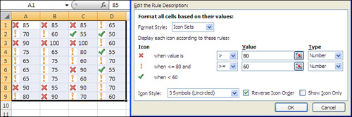
Sometimes, you might want to only apply a red X to the bad cells in a range. This is tricky to do in the user interface.
In the user interface, follow these steps to apply a red X to values greater than 80:
Add a three-symbols icon set to the range.
Specify that the symbols should be reversed.
Indicate that the third icon appears for values greater than
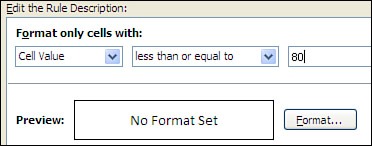
80. You now have a mix of all three icons, as shown in Figure 15.5.Add a new conditional format to highlight cells less than or equal to
80. Don’t specify any special formatting for the cells that match this rule, as shown in Figure 15.6.In the Conditional Formatting Rule Manager, indicate that Excel should stop evaluating conditions if the new condition is
true. This will prevent Excel from getting to the icon set rule for any cell with a value of80or less. The result is that only cells greater than80will appear with a red X, as shown in Figure 15.7.

The code to create this effect in VBA is fairly straightforward. A great deal of the code is spent making sure that the icon set has the red X symbols on the cells greater than 80.
When you use the FormatConditions.Add method to add the second condition, Excel initially refers to that condition as FormatConditions(2). However, you need to make sure this condition is executed first, so you use the SetFirstPriority method to move the new condition to the top of the list. The final step is to then turn on the StopIfTrue property; but you need to realize that the new condition is referred to as FormatConditions(1) after executing the SetFirstPriority method.
The code to highlight values greater than 80 with a red X is shown here:
Sub TrickyFormatting()
    With Range("A1:D9")
        .FormatConditions.Delete
        ' Add and format the 3 symbols icons
        .FormatConditions.AddIconSetCondition
        With .FormatConditions(1)
            .ReverseOrder = True
            .ShowIconOnly = False
            .IconSet = ActiveWorkbook.IconSets(xl3Symbols2)
        End With
        ' The threshhold for this icon doesn't really matter,
        ' but you have to make sure that it does not overlap the 3rd icon
        With .FormatConditions(1).IconCriteria(2)
            .Type = xlConditionValue
            .Value = 66
            .Operator = xlGreater
        End With
        ' Make sure the red X appears for cells above 80
        With .FormatConditions(1).IconCriteria(3)
            .Type = xlConditionValue
            .Value = 80
            .Operator = xlGreater
        End With

        ' Next, add a condition to catch items <=80
        .FormatConditions.Add Type:=xlCellValue, _
            Operator:=xlLessEqual, Formula1:="=80"
        ' Move this new condition from position 2 to position 1
        .FormatConditions(2).SetFirstPriority
        ' The new condition is now index #1. Add Stop if True.
        .FormatConditions(1).StopIfTrue = True
    End With
End SubThis trick is particularly cool because it can only be achieved with VBA. Say that values above 90 are acceptable and below 90 indicate trouble. You would like acceptable values to have a green bar and others to have a red bar.
Using VBA, you first add the green data bars. Then, without deleting the format condition, you add red data bars.
In VBA, every format condition has a Formula property that defines whether the condition is displayed for a given cell. So, the trick is to write a formula that defines when the green bars are displayed. When the formula is not True, the red bars are allowed to show through.
In Figure 15.8, the effect is being applied to range A1:D10. You need to write the formula in A1 style, as if it applies to the top-left corner of the selection. The formula needs to evaluate to True or False. Excel automatically copies the formula to all the cells in the range. The formula for this condition is =IF(A1>90,True,False).

Tip
The formula is evaluated relative to the current cell pointer location. Although it usually is not necessary to select cells before adding a FormatCondition, in this case, selecting the range ensures that the formula will work.
The following code creates the two-color data bars:
Sub AddTwoDataBars()
With Range("A1:D10")
.Select ' The .Formula below requires .Select here
.FormatConditions.Delete
' Add a Light Green Data Bar
.FormatConditions.AddDataBar
.FormatConditions(1).BarColor.Color = RGB(0, 255, 0)
.FormatConditions(1).BarColor.TintAndShade = 0.25
' Add a Red Data Bar
.FormatConditions.AddDataBar
.FormatConditions(2).BarColor.Color = RGB(255, 0, 0)
' Make the green bars only
.FormatConditions(1).Formula = "=IF(A1>90,True,False)"
End With
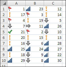
End SubThe Formula property works for all the conditional formats. This allows you to create some fairly obnoxious combinations of data visualizations. In Figure 15.9, five different icon sets are combined in a single range. Of course, no one would be able to figure out whether a red flag is worse than a gray down arrow, but this ability opens up interesting combinations for those with a little creativity.
Sub AddCrazyIcons()
    With Range("A1:C10")
        .Select ' The .Formula lines below require .Select here
        .FormatConditions.Delete

        ' First icon set
        .FormatConditions.AddIconSetCondition
        .FormatConditions(1).IconSet = ActiveWorkbook.IconSets(xl3Flags)
        .FormatConditions(1).Formula = "=IF(A1<5,TRUE,FALSE)"

        ' Next icon set
        .FormatConditions.AddIconSetCondition
        .FormatConditions(2).IconSet = ActiveWorkbook.IconSets(xl3ArrowsGray)
        .FormatConditions(2).Formula = "=IF(A1<12,TRUE,FALSE)"

        ' Next icon set
        .FormatConditions.AddIconSetCondition
        .FormatConditions(3).IconSet = ActiveWorkbook.IconSets(xl3Symbols2)
        .FormatConditions(3).Formula = "=IF(A1<22,TRUE,FALSE)"

        ' Next icon set
        .FormatConditions.AddIconSetCondition
        .FormatConditions(4).IconSet = ActiveWorkbook.IconSets(xl4CRV)
        .FormatConditions(4).Formula = "=IF(A1<27,TRUE,FALSE)"

        ' Next icon set
        .FormatConditions.AddIconSetCondition
        .FormatConditions(5).IconSet = ActiveWorkbook.IconSets(xl5CRV)
    End With
End SubAlthough the icon sets, data bars, and color scales get most of the attention, there are still plenty of other uses for conditional formatting.
The remaining examples in this chapter show off both some of the prior conditional formatting rules and some of the new methods available.
Use the AddAboveAverage method to format cells that are above or below average. After adding the conditional format, specify whether the AboveBelow property is xlAboveAverage or xlBelowAverage.
The following two macros highlight cells above and below average:
Sub FormatAboveAverage()
    With Selection
        .FormatConditions.Delete
        .FormatConditions.AddAboveAverage
        .FormatConditions(1).AboveBelow = xlAboveAverage
        .FormatConditions(1).Interior.Color = RGB(255, 0, 0)
    End With
End Sub

Sub FormatBelowAverage()
    With Selection
        .FormatConditions.Delete
        .FormatConditions.AddAboveAverage
        .FormatConditions(1).AboveBelow = xlBelowAverage
        .FormatConditions(1).Interior.Color = RGB(255, 0, 0)
    End With
End SubFour of the choices on the Top/Bottom Rules fly-out menu are controlled with the AddTop10 method. After you add the format condition, you need to set three properties that control how the condition is calculated:
TopBottom—. Set this to eitherxlTop10ToporxlTop10Bottom.Value—. Set this to5for the top 5,6for the top 6, and so on.Percent—. Set this toFalseif you want the top 10 item. Set this toTrueif you want the top 10 percent of the items.
The following code highlights top or bottom cells:
Sub FormatTop10Items()
    With Selection
        .FormatConditions.Delete
        .FormatConditions.AddTop10
        .FormatConditions(1).TopBottom = xlTop10Top
        .FormatConditions(1).Value = 10
        .FormatConditions(1).Percent = False
        .FormatConditions(1).Interior.Color = RGB(255, 0, 0)
    End With
End Sub

Sub FormatBottom5Items()
    With Selection
        .FormatConditions.Delete
        .FormatConditions.AddTop10
        .FormatConditions(1).TopBottom = xlTop10Bottom
        .FormatConditions(1).Value = 5
        .FormatConditions(1).Percent = False
        .FormatConditions(1).Interior.Color = RGB(255, 0, 0)
    End With
End Sub

Sub FormatTop12Percent()
    With Selection
        .FormatConditions.Delete
        .FormatConditions.AddTop10
        .FormatConditions(1).TopBottom = xlTop10Top
        .FormatConditions(1).Value = 12
        .FormatConditions(1).Percent = True
        .FormatConditions(1).Interior.Color = RGB(255, 0, 0)
    End With
End SubThe Remove Duplicates command on the Data tab of the Ribbon is a destructive command. You might want to mark the duplicates without removing them. If so, the AddUniqueValues method marks the duplicate or unique cells.
After calling the method, set the DupeUnique property to either xlUnique or xlDuplicate.
As I have ranted about in Special Edition Using Microsoft Office Excel 2007, I don’t quite like either option here. As you can see in Figure 15.10, choosing duplicate values, as in column A, marks both cells that contain the duplicate. For example, both A2 and A8 are marked, when really only A8 is the duplicate value.

Choosing unique values as in column B marks only the cells that don’t have a duplicate. This leaves several cells unmarked. For example, none of the cells containing 17 is marked.
As any data analyst knows, the truly useful option would have been to mark the first unique value. In this wishful state, Excel would mark one instance of each unique value. In this case, the 17 in E2 would be marked, but any subsequent cells that contain 17, such as E8, would remain unmarked.
Note
To achieve useful formatting in column E, see the HighlightFirstUnique code on page 391.
The code to mark duplicates or unique values is shown here:
Sub FormatDuplicate()
    With Selection
        .FormatConditions.Delete
        .FormatConditions.AddUniqueValues
        .FormatConditions(1).DupeUnique = xlDuplicate
        .FormatConditions(1).Interior.Color = RGB(255, 0, 0)
    End With
End Sub

Sub FormatUnique()
    With Selection
        .FormatConditions.Delete
        .FormatConditions.AddUniqueValues
        .FormatConditions(1).DupeUnique = xlUnique
        .FormatConditions(1).Interior.Color = RGB(255, 0, 0)
    End With
End SubThe value conditional formats have been around for several versions of Excel. Use the Add method with the following arguments:
Type—. In this section, the type will bexlCellValue.Operator—. Can bexlBetween,xlEqual,xlGreater,xlGreaterEqual,xlLess,xlLessEqual,xlNotBetween,xlNotEqual.Formula1—.Formula1is used with each of the operators specified to provide a numeric value.Formula2—. This is used forxlBetweenandxlNotBetween.
The following code sample highlights cells based on their values:
Sub FormatBetween10And20()
    With Selection
        .FormatConditions.Delete
        .FormatConditions.Add Type:=xlCellValue, Operator:=xlBetween, _
            Formula1:="=10", Formula2:="=20"
        .FormatConditions(1).Interior.Color = RGB(255, 0, 0)
    End With
End Sub

Sub FormatLessThan15()
    With Selection
        .FormatConditions.Delete
        .FormatConditions.Add Type:=xlCellValue, Operator:=xlLess, _
            Formula1:="=15"
        .FormatConditions(1).Interior.Color = RGB(255, 0, 0)
    End With
End SubWhen you are trying to highlight cells that contain a certain bit of text, you will use the Add method, the xlTextString type, and an operator of xlBeginsWith, xlContains, xlDoesNotContain, or xlEndsWith.
The following code highlights all cells that contain a capital letter A:
Sub FormatContainsA()
    With Selection
        .FormatConditions.Delete
        .FormatConditions.Add Type:=xlTextString, String:="A", _
            TextOperator:=xlContains
        ' other choices: xlBeginsWith, xlDoesNotContain, xlEndsWith
        .FormatConditions(1).Interior.Color = RGB(255, 0, 0)
    End With
End SubThe date conditional formats are new in Excel 2007. The list of available date operators is a subset of the date operators available in the new pivot table filters. Use the Add method, the xlTimePeriod type, and one of these DateOperator values: xlYesterday, xlToday, xlTomorrow, xlLastWeek, xlLast7Days, xlThisWeek, xlNextWeek, xlLastMonth, xlThisMonth, xlNextMonth.
The following code highlights all dates in the past week:
Sub FormatDatesLastWeek()
    With Selection
        .FormatConditions.Delete
        ' DateOperator choices include xlYesterday, xlToday, xlTomorrow,
        ' xlLastWeek, xlThisWeek, xlNextWeek, xlLast7Days
        ' xlLastMonth, xlThisMonth, xlNextMonth,
        .FormatConditions.Add Type:=xlTimePeriod, DateOperator:=xlLastWeek
        .FormatConditions(1).Interior.Color = RGB(255, 0, 0)
    End With
End SubBuried deep within the Excel interface are options to format cells that contain blanks, contain errors, do not contain blanks, or do not contain errors. If you use the macro recorder, Excel uses the complicated xlExpression version of conditional formatting. For example, to look for a blank, Excel will test to see whether the =LEN(TRIM(A1))=0. Instead, you can use any of these four self-explanatory types. You are not required to use any other arguments with these new types.
.FormatConditions.Add Type:=xlBlanksCondition
.FormatConditions.Add Type:=xlErrorsCondition
.FormatConditions.Add Type:=xlNoBlanksCondition
.FormatConditions.Add Type:=xlNoErrorsCondition
The most powerful conditional format is still the xlExpression type. In this type, you provide a formula for the active cell that evaluates to True or False. Make sure to write the formula with relative or absolute references so that the formula will be correct when Excel copies the formula to the remaining cells in the selection.
An infinite number of conditions can be identified with a formula. Two popular conditions are shown here.
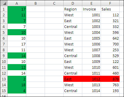
In column A of Figure 15.11, you would like to highlight the first occurrence of each value in the column. The highlighted cells will then contain a complete list of the unique numbers found in the column.
The macro should select cells A1:A15. The formula should be written to return a True or False value for cell A1. Because Excel logically copies this formula to the entire range, a careful combination of relative and absolute references should be used.
The formula can use the COUNTIF function. Check to see how many times the range from A$1 to A1 contains the value A1. If the result is equal to 1, the condition is True, and the cell is highlighted. The first formula is =COUNTIF(A$1:A1,A1)=1. As the formula gets copied down to, say A12, the formula changes to =COUNTIF(A$1:A12,A12)=1.
The following macro creates the formatting shown in column A of Figure 15.11:
Sub HighlightFirstUnique()
    With Range("A1:A15")
        .Select
        .FormatConditions.Delete
        .FormatConditions.Add Type:=xlExpression, _
            Formula1:="=COUNTIF(A$1:A1,A1)=1"
        .FormatConditions(1).Interior.Color = RGB(255, 0, 0)
    End With
End SubAnother example of a formula-based condition is when you want to highlight the entire row of a dataset in response to a value in one column. Consider the dataset in cells D2:F15 of Figure 15.11. If you want to highlight the entire row that contains the largest sale, you select cells D2:F15 and write a formula that works for cell D2: =$F2=MAX($F$2:$F$15). The code required to format the row with the largest sales value is as follows:
Sub HighlightWholeRow()
    With Range("D2:F15")
        .Select
        .FormatConditions.Delete
        .FormatConditions.Add Type:=xlExpression, _
            Formula1:="=$F2=MAX($F$2:$F$15)"
        .FormatConditions(1).Interior.Color = RGB(255, 0, 0)
    End With
End SubIn earlier versions of Excel, a cell that matched a conditional format could have a particular font, font color, border, or fill pattern. In Excel 2007, you can also specify a number format. This can prove useful for selectively changing the number format used to display the values.
For example, you might want to display numbers above 999 in thousands, numbers above 999,999 in hundred thousands, and numbers above 9 million in millions.
If you turn on the macro recorder and attempt to record setting the conditional format to a custom number format, the Excel 2007 VBA macro recorder actually records the action of executing an XL4 macro! Skip the recorded code and use the NumberFormat property as shown here:
Sub NumberFormat()
    With Range("E1:G26")
        .FormatConditions.Delete
        .FormatConditions.Add Type:=xlCellValue, Operator:=xlGreater, _
            Formula1:="=9999999"
        .FormatConditions(1).NumberFormat = "$#,##0,""M"""
        .FormatConditions.Add Type:=xlCellValue, Operator:=xlGreater,
            Formula1:="=999999"
        .FormatConditions(2).NumberFormat = "$#,##0.0,""M"""
        .FormatConditions.Add Type:=xlCellValue, Operator:=xlGreater,
            Formula1:="=999"
        .FormatConditions(3).NumberFormat = "$#,##0,K"
    End With
End Sub
Figure 15.12 shows the original numbers in columns A:C. The results of running the macro are shown in columns E:G. The dialog box shows the resulting conditional format rules.

In Chapter 16, “Reading from and Writing to the Web,” you will learn how to use Web queries to automatically import data from the Internet to your Excel applications.