The .NET class System.Diagnostics . Stopwatch can be used to measure elapsed time with roughly millisecond (0.001s) accuracy. This can be productively factored into a time combinator that accepts a function f and its argument x and times how long f takes to run when it is applied to x, returning a 2-tuple of the time taken and the result of f x:

> let time f x =
    let timer = new System.Diagnostics.Stopwatch()
    timer.Start()
    try f x finally
    printf "Took %dms" timer.ElapsedMilliseconds;;
val time : ('a -> 'b) -> 'a -> float * 'b

CPU time can be measured using a similar function.

The F# Sys .time function returns the CPU time consumed since the program began, and it can also be productively factored into a curried higher-order function cpu_time:

> let cpu_time f x =
    let t = Sys.time()
    try f x finally
    printf "Took %fs" (Sys.time() -. t);;
val cpu_time : ('a -> 'b) -> 'a -> float * 'b

CPU time can be measured with roughly centisecond (0.01s) accuracy using this function.

Many functions execute so quickly that they take an immeasurably small amount of time to run. In such cases, a higher-order loop function that repeats a computation many times can be used to provide a more accurate measurement:

> let rec loop n f x =
    if n > 0 then
      f x |> ignore
      loop (n - 1) f x;;
val loop : int -> ('a -> 'b) -> 'a -> 'b

For example, extracting the ll^th element of a list takes a very short amount of time:

> time (List.nth 10) [1 .. 100];;
Took 0ms
val it : int = 11

> time (loop 1000000 (List.nth 10)) [1 .. 100];;
Took 56 7ms
val it : int = 11

The former timing only allows us to conclude that the real time taken to fetch the 10^th element is < 0.001ms. The latter timing over a million repetitions allows us to conclude that the time taken is around 0.567µ s. The latter result is still erroneous because efficiency is often increased by repeating a computation (i.e. the first computation is likely to take longer than the rest) and the measurement did not account for the time spent in the loop function itself.

The time spent in the loop function can also be measured and turns out to be only 3% in this case:

> time (loop 1000000 (fun () -> ())) ();;
Took 17ms
val it : int = 11

The difference between real- and CPU-time is best elucidated by example.

The time and cpu_time combinators can be used to measure the absolute- and CPU-time required to perform a computation. In order to highlight the slower-passing of CPU time, we shall wrap the measurement of absolute time in a measurement of CPU time. Building a set from a sequence of integers is a suitable computation:

> cpu_time (time Set.of_seq) (seq {l .. 1000000});;
Took 4 719ms
Took 4.671875s
val it : Set<int> = seq [1; 2; 3; 4; ...]

The inner timing shows that the conversion of a million-element list into a set took 4.791s of real time. The outer timing shows that the computation and the inner timing consumed 4.67s of CPU time. Note that the outer timing returned a shorter time span than the inner timing, as CPU time passed more slowly than real time because the CPU was shared among other programs.

Timing a variety of equivalent functions is an easy way to quantify the performance differences between them. Choosing the most efficient functions is then the simplest approach to writing high-performance programs. However, timing individual functions by hand is no substitute for the complete profiling of the time spent in all of the functions of a program.

Although profiling is most useful when optimizing large programs that consist of many different functions, it is instructive to look at a simple example. Consider a program to solve the 8-queens problem. This is a logic problem commonly solved on computer science courses. The task is to find all of the ways that 8 queens can be placed on a chess board such that no queen attacks any other.

As this program makes heavy use of lists, it is useful to open the namespace of the List module:

> open List;;

A function safe that tests whether one position is safe from a queen at another position (and vice versa) may be written:

> let rec safe (xl, yl) (x2, y2) =
    xl <> x2 && yl <> y2 &&
      x2 - xl <> y2 - yl && xl - y2 <> x2 - yl;;
val safe : int * int -> int * int -> bool

A list of the positions on a n × n chess board may be generated using a list comprehension:

> let ps n =
    [for i in 1 .. n
       for j in 1 .. n ->
         i, j];;
val ps : int -> (int * int) list

A solution, represented by a list of positions of queens, may be printed to the console by printing a character for each position on a row followed by a newline, for each row:

> let print n qs =
    for x in 1 .. n do
      for y in 1 .. n do
        printf "%s" (if mem (x, y) qs then "Q" else ".")
      printf "
";;
val print : int -> (int * int) list -> unit

Solutions may be searched for by considering each safe position ps and recursing twice. The first recursion searches all remaining positions, returning the accumulated solutions accu. The second recursion adds a queen at the current position q and filters out all positions attacked by the new queen before recursing:

> let rec search f n qs ps accu =
    match ps with
    | [] when length qs = n -> f qs accu
    | [] -> accu
    | q::ps ->
        search f n qs ps accu;;
        |> search f n (q::qs) (filter (safe q) ps);;
val search :
  ((int * int) list -> 'a -> 'a) -> int ->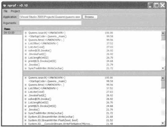

Figure 8.1. Profiling results generated by the freely-available NProf profiler for a program solving the queens problem on an 11 × 11 board.

(int * int) list -> (int * int) list -> 'a -> 'a

The search function is the core of this program. The approach used by this program, to recursively filter invalid solutions from a set of possible solutions, is commonly used in logic programming and is the foundation of some languages designed specifically for logic programming such as Prolog.

All solutions for a given board size n can be folded over using the search function. In this case, the fold prints each solution and increments a counter, finally returning the number of solutions found:

> let solve n =
    let f qs i =
      print n qs
      i + 1
    search f n [] (ps n) 0;;
val solve : int -> int

The problem can be solved for n = 8 and the number of solutions printed to the console (after the boards have been printed by the fold) with:

> printf "%d solutions
" (solve 8);;

This program takes only 0.15s to find and print the 92 solutions for n = 8. To gather more accurate statistics in the profiler, it is useful to choose a larger n. Using n = 11, compiling this program to an executable and running it from the NProf profiler gives the results illustrated in figure 8.1.

The profiling results indicate that almost 30% of the running time of the whole program is spent in the List. length function. The calls to this function can be completely avoided by accumulating the length nqs of the current list qs of queens as well as the list itself:

> let rec search f n nqs qs ps accu =
    match ps with
    | [] when nqs = n -> f qs accu
    | [] -> accu
    | q::ps ->
        search f n nqs qs ps accu
        |> search f n (nqs + 1) (q::qs)
             (filter (safe q) ps);;
val search :
  ((int * int) list -> 'a -> 'a) -> int -> int ->
    (int * int) list -> (int * int) list -> 'a -> 'a

The solve function just initializes with zero length nqs as well as the empty list:

> let solve n =
    let f qs i =
      print n qs;
      i + 1
    search f n 0 [] (ps n) 0;;
val solve : int -> int

This optimization reduces the time taken to compute the 2,680 solutions for n = 11 from 34.8s to 23.6s, a performance improvement of around 30% as expected.

Profiling can be used to identify the performance critical portions of whole programs. These portions of the program can then be targeted for optimization. Algorithmic optimizations are the most important set of optimizations.

The point at which asymptotic complexity ceases to be an accurate predictor of relative performance can be determined experimentally. This section presents experimental results illustrating some of the more important trade-offs and quantifying relevant performance characteristics on a test machine^[18].

Measuring the performance of functions in any setting, other than those in which the functions are to be used in practice, can easily produce misleading results. Al-though we have made every attempt to provide independent performance measure-ments, effects such as the requirements put upon the garbage collector by the different algorithms are always likely to introduce systematic errors. Consequently, the per-formance measurements which we now present must be regarded only as indicative measurements.

Figure 8.2 demonstrated that asymptotic algorithmic complexity is a powerful indicator of performance. In that case, testing for membership using Set. mem was found to be over 10⁶ × faster than List. mem for n = 10⁶. However, the relative performance of lists, arrays and sets was not constant over n and, in particular, arrays were the fastest container for small n. Figure 8.3 shows the ratio of the times taken to test for membership in small containers. For n < 35, arrays are up to twice as fast as sets.

Figure 8.3. Relative time taken t = t_s/t_a for testing membership in a set (ts) and an array (t a) as a function of the number of elements n in the container, showing that arrays are up to 2x faster for n < 35.

Figure 8.4. Measured performance (time t in seconds per element) of List. of _array, Array. copy and Set. of _array data structures containing n elements.

As this example illustrates, benchmarking is required when dealing with many operations on small containers.

Figure 8.4 illustrates the time taken to create a list, array or set from an array. Array creation is fastest, followed by list creation and then set creation. For 10³ elements on the test machine, creating a list element takes 16ns, an array element takes 6ns and a set element takes 1.9/µ s. Moreover, array creation takes an approximately-constant time per element regardless of the size of the resulting array whereas list and set creation takes longer per element for larger data structures, i.e. the total time taken to create an n -element list or set is not linear in n.

Figure 8.5. Measured performance (time t in seconds per element) of iter functions over list, array and set data structures containing n elements.

Although tests for membership and the set theoretic operations (union, intersection and difference) are asymptotically faster for sets than for lists and arrays, the fact that set creation is likely to be at least 300× slower limits their utility to applications that perform many elements lookups for every set creation. In fact, we shall study one such application of sets in detail in chapter 12.

Figure 8.5 illustrates the time taken to iterate over the elements of lists, arrays and sets. Iterating over arrays is fastest, followed by lists and then sets.

Iterating over a list is 4× slower than iterating over an array. The performance degredation for lists and sets when n is large is a cache coherency issue. Like most immutable data structures, both lists and sets allocate many small pieces of memory that refer to each other. These tend to scatter across memory and, consequently, memory access becomes the bottleneck when the list or set does not fit on the CPU cache. In contrast, arrays occupy a single contiguous portion of memory, so sequential access (e.g. iter) is faster for arrays. For example, iterating over a set is 8 × slower than iterating over an array for n = 10³ and 15 × slower for n = 10⁶.

Figure 8.6 illustrates the time taken to perform a left fold, summing the elements of a list, array or set in forward order. The curves are qualitatively similar to figure 8.5 for the iter functions but fold_left is up to 10× slower than iter.

Figure 8.7 illustrates the time taken to perform a right fold, summing the elements of a list, array or set. Left and right folds perform similarly for arrays and sets but lists show slightly different behaviour due to the stacking of intermediate results required to traverse the list in reverse order. Specifically, fold_right is 30% slower than fold_left for lists.

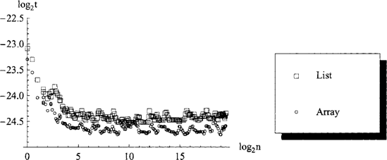
Figure 8.6. Measured performance (time t in seconds per element) of the fold_left functions over list and array data structures containing n elements.

Figure 8.7. Measured performance (time t in seconds per element) of the fold_right functions over list, array and set data structures containing n elements.

Figure 8.8. Controlling the optimization flags passed to the F# compiler by Visual Studio 2005.

These benchmark results may be used as reasonably objective, quantitative evi-dence to justify a choice of data structure. We shall now examine other forms of optimization, in approximately-decreasing order of productivity.

The simplest way to improve the performance of an F# program is to instruct the F# compiler to put more effort into optimizing the code. This is done by providing an optimization flag of the form -Ooff, −01, −02 or -03 where the latter instructs the compiler to try as hard as possible to improve the performance of the program.

In Visual Studio, the optimization setting for the compiler is controlled from the Project

As a last resort, program transformations performed manually should be consid-ered as a means of optimization. We shall now examine several different approaches. Although we try to associate quantitative performance benefits with the various ap-proaches, these are only indicative and are often chosen to represent the best-case.

Straightforward recursion is very efficient when used in moderation. However, the performance of deeply recursive functions can suffer. Performance degradation due to deep recursion can be avoided by performing tail recursion [16].

If a recursive function call is not tail recursive, state will be stored such that it may be restored after the recursive call has completed. This storing, and the subsequent retrieving, of state is responsible for the performance degradation. Moreover, the intermediate state is stored on a limited resource known as the stack which can be exhausted, resulting in StackOverflowException being raised.

Tail recursion involves writing recursive calls in a form which does not need this state. Most simply, a tail call returns the result of the recursive call directly, i.e. without performing any computation on the result.

For example, a function to sum a list of arbitrary-precision integers may be written:

> let rec sum = function
    | [] -> 0I
    | h::t -> h + sum t;;
val sum : bigint list -> bigint

Summing 10⁴ elements takes 2ms:

> time sum [1I .. 10000I];;
Took 2ms
val it : bigint = 50005000I

Attempting to sum 10⁵ elements exhausts stack space:

> time sum [1I .. 100000I]
Process is terminated due to StackOverflowException

The result of the recursive call sum t in the body of the sum function is not returned directly but, rather, has h added to it to create a new value that is then returned. Thus, this recursive call to sum is not a tail call.

The sum function can be written in tail recursive form by accumulating the sum in an argument and returning the accumulator when the end of the list is reached:

> let rec sum_tr_aux (accu : bigint) = function
    | [] -> accu
    | h::t -> sum_tr_aux (h + accu) t;;
val sum_tr_aux : bigint -> bigint list -> bigint

The signature of the auxiliary function sum_tr_aux is not the same as that of sum, as it must now be initialized with an accumulator of zero. A tail recursive sum_tr function can be written in terms of sum_tr_aux by applying zero as the initial accumulator:

> let sum_tr list =
    sum_tr_aux 0I list;;
val sum_tr : int list -> int

As this sum_tr function is tail recursive, it will not suffer from stack overflows when given long lists:

> time sum_tr [1I .. 10000I]
Took 8ms
val it : bigint = 50005000I

> time sum_tr [1I .. 100000I]
Took 47ms
val it : bigint = 5000050000I

> time sum_tr [1I . . 1000000I];;
Took 196ms
val it : bigint = 500000500000I

As we have seen, non-tail-recursive functions are not robust when applied to large inputs. However, many functions are naturally written in a non-tail-recursive form.

For example, the built-in List. fold_right function is most simply written as:

> let rec fold_right f list accu =
    match list with
    | [] -> accu
    | h::t -> f h (fold_right f t accu);;
val fold_right : ('a -> 'b -> 'b) -> 'a list -> 'b -> 'b

This form is not tail recursive. The built-in List. fold_right function is actually tail recursive, and tries to be efficient, but it still has an overhead compared to the List. fold_left function (see figures 8.6 and 8.7). The reason for this overhead stems from the fact that the fold_left function considers the elements in the list starting at the front of the list whereas the fold_right function starts at the back. On a container that allows random access, such as an array, there is little difference between considering elements in forward or reverse order. However, the primitive operation used to decompose a list presents the first element and the remaining list. Consequently, looping over lists is more efficient in forward order than in reverse order.

Many standard library functions suffer from the inefficiency that results from having been transformed into the more robust tail recursive form. In the List module, the fold_right, map, append and concat functions are not naturally tail recursive.

Although the .NET platform is based upon a common language run-time (CLR) that allows seamless interoperability between programs written in different languages, the platform has been optimized primarily for the C# language. As a conventional imperative language, C# programs have a typical value lifetime distribution that is significantly different to that of most functional programs. Specifically, functional programs often allocate huge numbers of short-lived small values and standalone functional programming languages like OCaml are optimized for this [11]. As .NET is not optimized for this, allocation in F# is more expensive and, consequently, optimizations that avoid allocation are correspondingly more valuable when trying to make F# programs run more quickly.

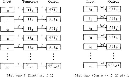
Figure 8.9. Deforestation refers to methods used to reduce the size of temporary data, such as the use of composite functions to avoid the creation of temporary data structures illustrated here: a) mapping a function f over a list 1 twice, and b) mapping the composite function f o f over the list 1 once.

Deforesting

Functional programming style often results in the creation of temporary data due to the repeated use of maps, folds and other similar functions. The reduction of such temporary data is known as deforestation. In particular, the optimization of performing functions sequentially on elements rather than containers (such as lists and arrays) in order to minimize the number of temporary containers created (illustrated in figure 8.9).

For example, the Shannon entropy H of a vector v representing a discrete proba-bility distribution is given by:

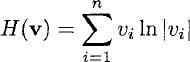
This could be written in F# by creating temporary containers, firstly u_i = 1n v_i and then w_i = u_iv_i and finally calculating the sum

> open List;;

> let entropyl v =
    fold_left (+) 0.0 (map2 (*) v (map log v));;

val entropyl : float list -> float

This function is written in an elegant, functional style by composing functions.

However, the subexpressions map log v for u and map2 (*) v (...) for w both result in temporary lists. Creating these intermediate results is slow. Specifically, the 0(n) allocations of all of the list elements in the intermediate results is much slower than any of the arithmetic operations performed by the rest of this function.

Fortunately, this function can be completely deforested by performing all of the arithmetic operations at once for each element, combining the calls to +, * and log into a single anonymous function:

> let entropy2 v =
    fold_left (fun hv->h+v* log v) 0.0 v;;
val entropy2 : float list -> float

Note that this function produces no intermediate lists, i.e. it performs only 0 (1) allocations.

The deforested entropy2 function is much faster than the entropyl function. For example, it is ~ 14 × faster when applied to a 10⁷-element list:

> time entropyl [1.0 .. 10000000.0];;
Took 13 971ms
val it : float = 7.809048631e+14

> time entropy2 [1.0 .. 10000000.0];;
Took 1045ms
val it : float = 7.809048631e+14

Deforesting can be a very productive optimization when using eager data structures such a lists, arrays, sets, maps, hash tables and so on. However, the map2 and map functions provided by the Seq module are lazy: rather than building an intermediate data structure they will store the function to be mapped and the original data structure. Thus, a third variation on the entropy function is deforested and lazy:

> let entropy3 v =
    Seq.map2 (*) v (Seq.map log v)
    |> Seq.fold (+) 0.0;;
val entropy3 : #seq<float> -> float

The performance of a lazy Seq-based implementation is between that of the deforested and forested eager implementations:

> time entropy3 [1.0 .. 10000000.0];;
Took 614 0ms
val it : float = 7.809048631e+14

Lazy functions are usually slower than eager functions so it may be surprising that the lazy entropy3 function is actually faster than the eager entropyl function in this case. The reason is that allocating large data structures is proportionally much slower than allocating small data structures. As the Seq. map function is lazy, the entropy3 function never allocates a whole intermediate list but, rather, allocates intermediate lazy lists. Consequently, the lazy entropy3 function evades the allocation and subsequent garbage collection of a large intermediate data structure and is twice as fast as a consequence.

The lazy implementation can also be deforested:

> let entropy4 v =
    Seq.fold (fun h v->h + v* log v) 0.0 v;;
val entropy4 : #seq<float> -> float

This deforested lazy implementation is faster than the forested lazy implementation but not as fast as the deforested eager implementation:

> time entropy4 [1.0 .. 10000000.0];;
Took 216 7ms
val it : float = 7.809048631e+14

The deforested eager entropy2 function is the fastest implementation because it avoids the overheads of both intermediate data structures and laziness. Consequently, this style should be preferred in performance-critical code and, fortunately, it is easy to write in F# thanks to first-class functions and the built-in function composition operators.

> let f = function
    | 0, _ | _, 0 -> 0, 0
    | x, y -> x, y;;
val f : int * int -> int * int

> let f = function
    | 0, _ | _, 0 -> 0, 0
    | a - > a;;
val f : int * int -> int * int

> let rec sortl = function
    | [] -> []
    | X::XS ->
        match sortl xs with
        | y::ys when x > y -> y::sortl(x::ys)
        | ys -> X::ys;;
val sortl : 'a list -> 'a list

> let rec sort2 = function
    | [] -> []
    | x::xs as list ->
        match sort2 xs with
        | y::ys when x > y -> y::sort2(x::ys)
        | ys -> if xs == ys then list else x::ys;;
val sort2 : 'a list -> 'a list

Algorithms may execute more quickly if they can avoid unnecessary computation by terminating as early as possible. However, the trade-off between any extra tests required and the savings of exiting early can be difficult to predict. The only general solution is to try premature termination when performance is likely to be enhanced and revert to the simpler form if the savings are not found to be significant. We shall now consider a simple example of premature termination as found in the core library as well as a more sophisticated example requiring the use of exceptions.

The for_all function in the List module is an enlightening example of an early-terminating function. This function applies a predicate function p to elements in a list, returning true if the predicate was found to be true for all elements and false otherwise. Note that the predicate need not be applied to all elements in the list, as the result is known to be false as soon as the predicate returns false for any element. The for_all function may be written:

> let rec for_alll p = function
    | [] -> true

| h::t -> p h && for_alll p t;;
val for_alll : ('a -> bool) -> 'a list -> bool

The premature termination of this function is not immediately obvious. In fact, the && operator has the unusual semantics of in-order, short-circuit evaluation. This means that the expression p h will be evaluated first and only if the result is true will the expression for_a111 p tbe evaluated. Consequently, this implementation of the for_al1 function can return false without recursively applying the predicate function p to all of the elements in the given list.

Moreover, the short-circuit evaluation semantics of the && operator makes the above function equivalent to:

> let rec for_alll p = function
    | [] -> true
    | h::t -> if p h then for_alll p t else false;;
val for_alll : ('a -> bool) -> 'a list -> bool

Consequently, these for_all functions are actually tail recursive (the result of the call for_al1 p t is returned without being acted upon).

These implementations of the for_all function are very efficient. Terminating on the first element takes under 50ns:

> [1 . . 1000]
  |> time (loop 100000 (for_alll ((<>) 1)));;
Took 5ms
val it : bool = false

Terminating on the 1000^th element takes 11µ s:

> [1 . . 1000]
  |> time (loop 100000 (for_alll ((<>) 1000)));;
Took 1144ms
val it : bool = false

These performance results will now be used to compare an alternative exit strategy: exceptions.

A similar function may be written in terms of a fold:

> let for_all2 p list =
    List.fold_left (&&) true list;;
val for_all : ('a -> bool) -> 'a list -> bool

However, this for_a112 function will apply the predicate p to every element of the list, i.e. it will not terminate early.

The fold-based implementation can be made to terminate early by raising and catching an exception:

> let for_a113 p list =
    try
      let f b h = p h && raise Exit

List.fold_left f true list
    with
    | Exit ->
        false;;
val for_all3 : ('a -> bool) -> 'a list -> bool

Indeed, there is now no reason to accumulate a boolean that is always true. The function can be written using iter or a comprehension instead of a fold:

> let for_all4 p list =
    try
      for h in list do
        if not (p h) then raise Exit
      true
    with
    | Exit ->
        false;;
val for_all4 : ('a -> bool) -> 'a list -> bool

This function has recovered the asymptotic efficiency of the original for_alll function but the actual performance of this for_a114 function cannot be determined without measurement. Indeed, as exceptions are comparatively slow in .NET the exception-based approach is likely to be significantly slower when the exception is raised and caught.

When terminating on the first element, the performance is dominated by the cost of raising and catching an exception. The time taken to return at the first element is 29 µ s:

> [1 . . 1000];;
  |> time (loop 100000 (for_all4 ((<>) 1)));;
Took 2862ms
val it : bool = false

Terminating on the 1000^th element takes 43µ s:

> [1 . . 1000];;
  |> time (loop 100000 (for_all4 ((<>) 1000)));;
Took 426 9ms
val it : bool = false

In the latter case, a significant amount of other computation is performed and the performance cost of the exception is not too significant. Consequently, the for_all4 function is 4×slower than the original for_alll function. However, if the flow involves a small amount of computation and an exception, as it does in the former case, then the exceptional route is 600 × slower. This is such a signifi-cant performance difference that the standard library provides alternative functions for performance critical code that avoid exceptions in all cases. For example, the assoc and find functions in the List module have try_assoc and try find alternatives that return an option result to avoid raising an exception when a result is not found.

In F#, applying functions as arguments can lead to slower code. Consequently, avoiding higher-order functions in the primitive operations of numerically-intensive algorithms can significantly improve performance.

For example, a function to sum an array of floating point numbers may be written in terms of a fold:

> let suml a =
    Array.fold_left (+) 0.0 a;;
val suml : float array -> float

Alternatively, the function may be written using an explicit loop rather than a fold:

> let sum2 a =
    let r = ref 0.0
    for i = 0 to Array.length a - 1 do
      r := !r + a. [i]
    !r;;
val sum2 : float array -> float

Clearly, the fold has significantly reduced the amount of code required to provide the required functionality.

The overhead of using a higher-order function results in the suml function exe-cuting significantly more slowly than the sum2 function:

> let a = Array.init 10000000 float;;
val a : float array

> time suml a;;
Took 3 76ms
val it : float = 4.9999995el3

> time sum2 a;;
Took 104ms
val it : float = 4.9999995el3

In this case, the sum2 function is 3.6× faster than the suml function. In fact, performance can be improved even more by using a mutable value.

The mutable keyword can be used in a let binding to create a locally mutable value. Mutable values are not allowed to escape their scope (e.g. they cannot be used inside a nested closure). However, mutable values can be more efficient than references.

For example, the previous section detailed a function for summing the elements of a float array. The fastest implementation used a reference for the accumulator but this can be written more efficiently using a mutable:

> let sum3 a =
    let mutable r = 0.0
    for i = 0 to Array.length a - 1 do
      r <- r + a. [i] r;;
val sum3 : float array -> float

Using a mutable makes this sum3 function 2.7×faster than the fastest previous implementation sum2 that used a reference:

> time sum3 a;;
Took 3 9ms
val it : float = 4.9999995el3

The combination of avoiding higher-order functions and using mutable makes this sum3 function 9.6 × faster than the original suml.

Particularly in the context of scientific computing, F# programs can benefit from the use of specialized high-performance functions. This includes some complicated numerical algorithms for matrix and Fourier analysis, which will be covered in chapter 9, but the F# standard library also provides some fast functions for common mathematical values.

The built-in vector type implements arbitrary-dimensionality vectors with float elements and provides operators that are considerably faster than equivalent functions from the Array module:

> let a, b = [|1.0 .. 1000.0|], [|l.O .. 1000.0 |];;
val a : float array
val b : float array

> time (loop 100000 (Array.map2 (+) a)) b
     |> ignore;;
Took 5744ms
val it : unit = ()

> (vector a, vector b)
     |> time (loop 100000 (fun (a, b) -> a + b))
     |> ignore;;
Took 2 014ms
val it : unit = ()

In this case, vector addition is 2.9 × faster using the specialized vector addition.

Figure 8.10. An array of tuples or records containing pairs of float values incurs a level of indirection.

Figure 8.11. A struct can be used to completely unbox the float values, placing them directly into the array. This is often the most efficient representation.

Typically in functional languages, most values are boxed. This means that a value is stored as a reference to a different piece of memory. Although elegant in pro-viding efficient referential transparency, unnecessary boxing can incur significant performance costs.

For example, much of the efficiency of arrays stems from their elements occupying a contiguous portion of memory and, therefore, accesses to elements with similar indices are cache coherent. However, if the array elements are boxed, only the references to the data structures will be in a contiguous portion of memory (see figure 8.10). The data structures themselves may be at completely random locations, particularly if the array was not filled sequentially. Consequently, cache coherency may be very poor.

For example, computing the product of an array of complex numbers is unnec-essarily inefficient when the numbers are represented by a (float * float) array (see figure ??). A struct is often more efficient as this avoids all unboxing (see figure 8.11).

A function to compute the product of an array of complex numbers might be written over the type (float * float) array, where each element is a 2-tuple representing the real and imaginary parts of a complex number:

> let productl zs =
    let mutable re = 1.0
    let mutable im = 0.0
    for i = 0 to Array.length zs - 1 do
      let zr, zi = zs.[i]
      let r = re * zr - im * zi
      and i = re * zi + im * zr
      re <- r

im <- i
    re, im;;
val productl : (float * float) array -> float * float

To avoid boxing completely, the complex number can be stored in a struct:

> type Complex = struct
    val re : float
    val im : float
    newfx, y) = { re = x; im = y }
  end;;

A more efficient alternative may act upon values of the type Complex array:

> let product2 (zs : Complex array) =
    let mutable re = 1.0
    let mutable im = 0.0
    for i = 0 to Array.length zs - 1 do
      let r = re * zs.[i].r - im * zs.[i].i
      and i = re * zs.[i].i + im * zs.[i].r
      re <- r
      im <- i
    re, im;;
val product2 : Complex array -> float * float

Benchmarking these two functions compiled to native code with full compiler optimizations and acting upon randomly shuffled 2²⁴-element arrays, we find that the tuple-based productl function takes 1.94s to complete and the struct-based product 2 function takes only 0.25s.

The definition of a local function or the partial application of a curried function can create a closure. This functionality is not provided by the .NET platform and, con-sequently, F# must distinguish between the types of ordinary functions and closures to remain compatible. The type of a closure is bracketed, so ' a - > ' b becomes ('a -> 'b).

For example, both of the following functions compute the next integer and may be used equivalently in F# programs but the former is an ordinary function (like a C# function) whereas the latter is a closure that results from partial application of the curried + function:

> let succ1 n =
    n + 1;;
val succl : int -> int

> let succ2 =
    (+) 1;;
val succ2 : (int -> int)

Closures encapsulate both a function and its environment (such as any partially applied arguments). Consequently, closures are heavier than functions and the cre-ation and invocation of a closure is correspondingly slower. In fact, the F# compiler translates a closure into an object that encapsulates the environment and function.

The F# programming language provides an inline keyword that provides a simple way to inline the body of a function at its calls sites:

> let f x y = x + y;;
val f : int -> int -> int

> let inline f x y = x + y;;
val f : ^a -> ^b -> ^c when ^a :
  (static member (+) : ^a -> ^b -> ^c)

The body of the function marked inline will be inserted verbatim whenever the function is called. Note that the type of the inlined function is very different. This is because ordinary functions require ad-hoc polymorphic functions such as the + operator to be ossified to a particular type, in this case the default type int. In contrast, the inlining of the function in the latter case allows the body of the function to adopt whatever type is inferred from any context it is inserted into individually. Hence its type requires only that a + operator is defined in the context of the call site.

The performance implications of inlining vary wildly, with numeric code often benefitting from judicious inlining but the performance of symbolic code is often deteriorated by inlining.

The F# input_value and output_value functions or the standard .NET serialization routines themselves can be used to store and retrieve arbitrary data using a binary format. However, at the time of writing these routines in the .NET library are not optimized and require as much space as a textual format and often take several times as long as a custom parser to load. In particular, the current .NET serialization implementation has quadratic complexity when serializing data structures containing many shared functions. This includes the serialization of data structures that contain INumeric implementations, such as the F# vector and matrix types.

Consequently, programs with performance limited by IO may be written more efficiently by handling custom formats, such as textual representations of data (parsed using the techniques described in chapter 5) or even using a custom binary format. CPU performance has increased much more quickly than storage performance and, as a consequence, data compression can sometimes be used to improve IO performance by reducing the amount of data being stored in exchange for a higher CPU load.

Having examined the many ways F# programs may be optimized, we shall now review existing libraries which may be of use to scientists.