Chapter 15
Understand and design indexes
This chapter dives into indexing of all kinds—not just clustered and nonclustered indexes—including practical development techniques for designing indexes. It mentions memory-optimized tables throughout, including hash indexes for extreme writes and columnstore indexes for extreme reads. The chapter reviews missing indexes and index usage, and then introduces statistics—how they are created and updated. There are important performance-related options for statistics objects. Finally, it explains special types of indexes for niche uses.
In SQL Server you have access to a variety of indexing tools in your toolbox.
We’ve had clustered and nonclustered indexes in all 21st-century versions of SQL Server—those two rowstore index types that are the bread and butter of SQL Server. We cover those in the first half of this chapter, including important new options for SQL Server 2022.
Introduced in SQL Server 2012, columnstore indexes presented a new and exciting way to perform analytical queries on massive amounts of compressed data. They became an essential tool for database developers, and this chapter discusses them in detail. SQL Server 2014 brought memory-optimized tables and their uniquely powerful hash indexes for latchless querying on rapidly changing data. You can even combine the power of these two new concepts now, with columnstore index concepts on memory-optimized tables, allowing for live analytical-scale queries on streamed data. First, though, we’re going to dive into the index design concepts.
All scripts for this book are all available for download at https://www.MicrosoftPressStore.com/SQLServer2022InsideOut/downloads.
Design clustered indexes
Let’s be clear about what a clustered index is, and then state the case for why every table in a relational database should have one, with very few exceptions.
First, we will discuss rowstore clustered indexes. It is also possible to create a clustered columnstore index. We discuss that later in this chapter.
Whether you are inheriting and maintaining a database or designing the objects within it, there are important facts to know about clustered indexes. In the case of both rowstore and columnstore indexes, the clustered index stores the data rows for all columns in the table. In the case of rowstore indexes, the table data is logically sorted by the clustered index key; in the case of clustered columnstore indexes, there is no key. Memory-optimized tables don’t have a clustered index structure inherent to their design but could have a clustered columnstore index created for them.
Choose a proper rowstore clustered index key
There are four marks of a good clustered index key for most OLTP applications, or in the case of a compound clustered index key, the first column listed. The column order matters. Let’s review four key factors that will help you understand what role the clustered index key serves, and how best to design one:
Increasing sequential value. A value that increases with every row inserted (such as 1,2,3…, or an increasing point in time, or an increasing alphanumeric) is useful in efficient page organization. This means the insert pattern of the data as it comes in from the business will match the loading of rows onto the physical structures of the table.
A column with the
identityproperty, or populated by a value from a sequence object, matches this perfectly. Use date and time data only if it is highly unlikely to repeat, and then strongly consider using thedatetimeoffsetdata type to avoid repeated data once annually during daylight saving time changes.Unique. A clustered index key does not need to be unique, but in most cases it should be. (The clustered key also does not need to be the primary key of the table, or the only uniqueness enforced in the table.) A unique (or near-unique) clustered index means efficient seeks. If your application will be searching for individual rows out of this table regularly, you and the business should know what makes those searches unique.
Unique constraints, whether nonclustered or clustered, can improve performance on the same data and create a more efficient structure. A unique constraint is the same as a unique rowstore nonclustered index.
If a clustered index is declared without the
UNIQUEproperty, a second key value is added in the background: a four-byte integer uniquifier column. SQL Server must have some way to uniquely identify each row. The key from the rowstore clustered index is used as the row locator for nonclustered indexes, which leads to the next factor.Nonchanging. Choose a key that doesn’t change, and is a system-generated key that shouldn’t be visible to end-user applications or reports. In general, when end users can see data, they will eventually see fit to change that data. You do not want clustered index keys to ever change (much less
PRIMARY KEYvalues). A system-generated or surrogate key of sequential values (like anIDENTITYcolumn) is ideal. A field that combines system or application-generated fields such as dates and times or numbers would work too.The negative impact of changing the clustering key includes the possibility that the first two aforementioned guidelines would be broken. If the clustered key is also a primary key, updating the key’s values could also require cascading updates to enforce referential integrity. It is much easier for everyone involved if only columns with business value are exposed to end users and, therefore, can be changed by end users. In normalized database design, we would call these natural keys as opposed to surrogate keys.
Narrow data type. The decision with respect to data type for your clustered index key can have a large impact on table size, the cost of index maintenance, and the efficiency of queries at scale. The clustered index key value is also stored with every nonclustered index key value, meaning that an unnecessarily wide clustered index key will also cause unnecessarily wide nonclustered indexes on the table. This can have a very large impact on storage on drives and in memory at scale.
The narrow data type guidance should also steer you away from using the
uniqueidentifierfield, which is 16 bytes per row, or four times the size of an integer column per row, and twice as large as abigint. It also steers away from using wide strings, such as names, addresses, or URLs.
The clustered index is an important decision in the structure of a new table. For the vast majority of tables designed for relational database systems, however, the decision is fairly easy. An identity column with an INT or BIGINT data type is the ideal key for a clustered index because it satisfies the aforementioned four recommended qualities of an ideal clustered index. A procedurally generated timestamp or other incrementing time-related value, combined with a unique, autoincrementing number, also provides for a common, albeit less-narrow, clustered index key design.
When a table is created with a primary key constraint and no other mention of a clustered index, the primary key’s columns become the clustered index’s key. This is typically safe, but a table with a compound primary key or a primary key that does not begin with a sequential column could result in a suboptimal clustered index. It is important to note that the primary key does not need to be the clustered index key, but often should be. It is possible to create nonunique clustered indexes or to have multiple unique columns or column combinations in a table.
When combining multiple columns into the clustered index key, keep in mind that the column order of an index, clustered or nonclustered, does matter. If you decide to use multiple columns to create a clustered index key, the first column should still align as closely to the other three rules, even if it alone is not unique.
In the sys.indexes catalog view, the clustered index is always identified as index_id = 1. If the table is a heap, there will instead be a row with index_id = 0. This row represents the heap data.
The case against intentionally designing heaps
Without a clustered index, a table is known as a heap. In a heap, the Database Engine uses a structure known as row identifier (RID), which uniquely identifies every row for internal purposes. The structure of the heap has no order when it is stored. RIDs do not change, so when a record is updated, a forwarding pointer is created in the old location to point to the new. Also, if the row that has the forwarding pointer is moved to another page, it gets another forwarding pointer. Even deleted rows can have forwarding pointers! If that sounds like it is complicated or would increase the amount of I/O activity needed to store and retrieve the data, you’re right.
Furthering the performance problems associated with heaps are that table scans are the only method of access to read from a heap structure, unless a nonclustered index is created on the heap. It is not possible to perform a seek against a heap; however, it is possible to perform a seek against a nonclustered index that has been added to a heap. In this way, a nonclustered index can provide an ordered copy for some of the table data in a separate structure.
One edge case for designing a table purposely without a clustered index is if you would only ever insert into a table. Without any order to the data, you might reap some benefits from rapid, massive data inserts into a heap. Other types of writes to the table (deletes and updates) will likely require table scans to complete and likely be far less efficient than the same writes against a table with a clustered index.
Deletes and updates typically leave wasted space within the heap’s structure, which cannot be reclaimed even with an index rebuild operation. To reclaim wasted space inside a heap without re-creating it, you must, ironically, create a clustered index on the table, then drop the clustered index. You can also use the ALTER TABLE ... REBUILD Transact-SQL (T-SQL) command to rebuild the heap.
The perceived advantage of heaps for workloads exclusively involving inserts can be easily outweighed by the significant disadvantages whenever accessing that data—when query performance would necessitate the creation of a clustered and/or nonclustered index. Table scans and RID lookups for any significant number of rows are likely to dominate the cost of any execution plan accessing the heap. Without a clustered index, queries reading from a table large enough to gain significant advantage from its inserts would perform poorly.
Microsoft’s expansion into modern unstructured data platforms, including integration with Azure Data Lake Storage Gen2, S3-compatible storage, Apache Spark, and other architectures, is likely to be more appropriate when rapid, massive data inserts are required. This is especially true for when you will continuously collect massive amounts of data and then only ever analyze the data in aggregate. These alternatives, integrated with the Database Engine starting with SQL Server 2016, or a focus of new Azure development such as Azure Synapse, would be superior to intentionally designing a heap.
Further, adding a clustered index to optimize the eventual retrieval of data from a heap is nontrivial. Behind the scenes, the Database Engine must write the entire contents of the heap into the new clustered index structure. If any nonclustered indexes exist on the heap, they also will be re-created, using the clustered key instead of the RID. This will likely result in a large amount of transaction log activity and tempdb space being consumed.
Understand the OPTIMIZE_FOR_SEQUENTIAL_KEY feature
Earlier in this chapter, we sang the praises of a clustered index key with an increasing sequential value, such as an integer based on an identity or sequence. For very frequent, multithreaded inserts into a table with an identity or sequence, the “hot spot” of the page in memory with the “next” value can provide some I/O bottleneck. (Long term, this is still likely preferable to fragmentation-upon-insertion, as explained in the previous section, and only surfaces at scale.)
A useful feature introduced in SQL Server 2019 is the OPTIMIZE_FOR_SEQUENTIAL_KEY index option, which improves the concurrency of the page needing rapid inserts for rowstore indexes from multiple threads.
You might observe a high amount of the PAGELATCH_EX wait type on sessions performing inserts into the same table. You can observe this with the dynamic management view (DMV) sys.dm_exec_session_wait_stats, or at an instance aggregate level with sys.dm_os_wait_stats. You should see this wait type drop when the new OPTIMIZE_FOR_SEQUENTIAL_KEY index option is enabled on indexes in tables that are written to by multiple requests simultaneously. Note that this isn’t the PAGEIOLATCH_EX wait type, more associated with physical page contention, but PAGELATCH_EX, associated with memory page contention.
 For more information on observing wait types with DMVs, including the differences between the
 PAGEIOLATCH_EXandPAGELATCH_EXwait types, see Chapter 8.
Let’s take a look at implementing OPTIMIZE_FOR_SEQUENTIAL_KEY. In our contrived example, multiple T-SQL threads frequently executing single-row inserting statements mean that the top two predominant wait types accrued via the DMV sys.dm_os_wait_stats are WRITELOG and PAGELATCH_EX. As Chapter 8 explained, the WRITELOG wait type is fairly self-explanatory—sending data to the transaction log—while PAGELATCH_EX is an indication of a “hot spot” page, symptomatic of rapid concurrent inserts into a sequential key.
By enabling OPTIMIZE_FOR_SEQUENTIAL_KEY on your rowstore indexes—both clustered and nonclustered—you should see some reduction in PAGELATCH_EX and the introduction of a small amount of a new wait type, BTREE_INSERT_FLOW_CONTROL, which is associated with the new OPTIMIZE_FOR_SEQUENTIAL_KEY setting.
Note
The new OPTIMIZE_FOR_SEQUENTIAL_KEY option is not available when creating columnstore indexes or for any indexes on memory-optimized tables.
You can query the value of the OPTIMIZE_FOR_SEQUENTIAL_KEY option with a new column added to sys.indexes of the same name. Note that this new option is not enabled by default, so it must be enabled manually on each index. The option is retained after an index is disabled and then rebuilt. For existing rowstore indexes, you can change the new OPTIMIZE_FOR_SEQUENTIAL_KEY option without a rebuild operation, with the following syntax:
ALTER INDEX PK_table1 on dbo.table1
SET (OPTIMIZE_FOR_SEQUENTIAL_KEY = ON);
Note
There are only a handful of index settings that can be set like this without a rebuild operation, so the syntax might look a little unusual. The index options ALLOW_PAGE_LOCKS, ALLOW_ROW_LOCKS, OPTIMIZE_FOR_SEQUENTIAL_KEY, IGNORE_DUP_KEY, and STATISTICS_NORECOMPUTE can be set without a rebuild.
Design rowstore nonclustered indexes
Each table almost always should have a clustered index that both defines the order and becomes the data structure of the data in the table. Nonclustered indexes provide additional copies of the data in vertically filtered sets, sorted by nonprimary columns.
You should approach the design of nonclustered indexes in response to application query usage, and then verify over time that you are benefitting from indexes. (You can read more about index usage statistics later in this chapter.) You might also choose to design a unique rowstore nonclustered index to enforce a business constraint. A unique constraint is implemented in the same way as a unique rowstore nonclustered index. This might be a valuable part of the table’s behavior even if the resulting unique rowstore nonclustered index is never queried.
Here are the properties of ideal nonclustered indexes:
Broad enough to serve multiple queries, not just designed to suit one query.
Well-ordered keys eliminate unnecessary sorting in high-value queries.
Well-stocked
INCLUDEsections prevent lookups in high-value queries, but can become out of control if too much value without investigation is given to the missing index DMVs.Proven beneficial usage over time in the
sys.dm_db_index_usage_statsDMV.Unique when possible (keep in mind a table can have multiple uniqueness criteria).
Key column order matters, so in a compound index, it is likely best for the most selective (with the most distinct values) columns to be listed first.
Nonclustered indexes on disk-based tables are subset copies of a rowstore table that take up space on storage and in memory. (On memory-optimized tables, indexes interact with the disk much differently. More on that later in this chapter.) You must spend time maintaining all nonclustered indexes. They are kept transactionally consistent with the data in the table, serving a limited, reordered set of the data in a table. All writes (including deletes) to the table data must also be written to the nonclustered index (in the case of updates, when any indexed column is modified) to keep it up to date. (On columnstore optimized tables, this happens a little differently, with a delta store of change records.)
The positive benefit rowstore nonclustered indexes can have on SELECT, UPDATE, and DELETE queries that don’t use the clustered index, however, is potentially very significant. Keep in mind that some write queries might appear to perform more quickly because accessing the data that is being changed can be optimized, as with accessing the data in a SELECT query. Your applications’ writes will slow with the addition of nonclustered indexes, and adding many nonclustered indexes will certainly contribute to poor write performance. You can be confident that creating any one well-designed nonclustered index will contribute to reads greatly, and not have a perceivable impact on writes.
You should not create nonclustered indexes haphazardly or clumsily; you should plan, modify, combine them when appropriate, and review them regularly to make sure they are still useful. (See the section “Understand and provide index usage” later in this chapter.) However, nonclustered indexes represent a significant source of potential performance tuning that every developer and database administration should be aware of, especially in transactional databases. Remember: Always look at the “big picture” when creating indexes. Very rarely does a single query rise to the level of importance of justifying its own indexes.
Note
Starting with SQL Server 2019, the RESUMEABLE syntax can be used when creating an index with the ONLINE syntax. An ALTER INDEX and CREATE INDEX statement can be similarly paused and resumed. For more on RESUMABLE index maintenance, see Chapter 8.
Understand nonclustered index design
Let’s talk about what we meant a moment ago when we said, “You should not create nonclustered indexes haphazardly or clumsily.” When should you create a nonclustered index, and how should you design them? How many should you add to a table?
Even though adding nonclustered indexes on foreign key columns can be beneficial if those referencing columns will frequently be used in queries, it’s rare that a useful nonclustered index will be properly designed with a single column in mind. This is because outside of joins on foreign keys, it is rare that queries will be designed to both seek and return a single column from a table. Starting a database design with indexes on foreign key columns is useful; that doesn’t mean, however, that they can’t be changed to have more columns at the end of the key list or in the include list.
Further, nonclustered rowstore index design should always be aware of all the indexes on a table and looking for opportunities to combine indexes with overlapping keys. In the next section, we’ll talk about index keys and overlapping index keys.
Choose a proper index
When creating new nonclustered indexes for a table, you must always compare the new index to existing indexes. The order of the key of the index matters. In T-SQL, it looks like this:
CREATE NONCLUSTERED INDEX IDX_NC_InvoiceLines_InvoiceID_StockItemID
ON [Sales].[InvoiceLines] (InvoiceID, StockItemID);
In this index, InvoiceID and InvoiceLineID are defined as the key. Using Object Explorer in SQL Server Management Studio (SSMS), you can view the index properties to see the same information. This nonclustered index represents a copy of two of the columns of data in the InvoiceLines table, sorted by the column InvoiceID first, and then the StockItemID. Neither of these columns are the primary key or the first key of the clustered index, which we can assume is InvoiceLineID.
To emphasize that the order of key columns in a nonclustered index matters, the two indexes that follow are completely different structures, and will best serve different queries. It’s unlikely that a single query would have much use for both nonclustered indexes, though SQL Server can still choose to use an index with less-than-optimal key order rather than scan a clustered index:
CREATE INDEX IDX_NC_InvoiceLines_InvoiceID_StockItemID
ON [Sales].[InvoiceLines] (InvoiceID, StockItemID);
CREATE INDEX IDX_NC_InvoiceLines_StockItemID_InvoiceID
ON [Sales].[InvoiceLines] (StockItemID, InvoiceID);
The columns with the most distinct values are more selective and will usually best serve queries if they are listed before less-selective columns in the index order. Note, though, that the order of columns in the INCLUDE portion of a nonclustered index (more on that later) does not matter.
Remember also from the previous section on clustered indexes that the clustered index key is already inside the key of the nonclustered index. There might be scenarios when the missing indexes feature (more on this later) suggests adding a clustered key column to your nonclustered index. It does not change the size of a nonclustered index to do this; the clustered key is already in a nonclustered index. The only caveat is that the order of the nonclustered index keys still determines the sort order of the index. So, having the clustered index key column(s) in your nonclustered index key won’t change the index’s size, but could change the sort order of the keys, creating what is essentially a different index when compared to an index that doesn’t include the clustered index key column(s).
The default sort order for index column values is ascending. If you want to sort in descending order, you must be explicit in that as in the query that follows. If queries frequently call for data to be sorted by a column in descending order, which might be common for queries looking for the most recent data, you could provide that key value like this:
CREATE INDEX IDX_NC_InvoiceLines_InvoiceID_StockItemID
ON [Sales].[InvoiceLines] (InvoiceID DESC, StockItemID);
Creating the key’s sort order incorrectly might not matter to some queries. For example, the nested loop operator does not require data to be sorted in a particular order, so different sort orders in the keys of a nonclustered index might not make a significant impact to the execution plan. On the other hand, a merge join operator requires data in both inputs to the operator to be sorted in the same order, so changing the sort order of the keys of an index—especially the first key—could simplify an execution plan by eliminating unnecessary sort operators. This is among the strategies of index tuning to consider. Remember to review the query plan performance data that the Query Store collects to observe the impact of index changes on multiple queries.
- For more on performance tuning, see Chapter 14, “Performance tune SQL Server.”
Understand redundant indexes
Nonclustered index keys shouldn’t overlap with other indexes in the same table. Because index key order matters, you must be aware of what is and what isn’t an overlapping index. Consider the following two nonclustered indexes on the same table:
CREATE INDEX IDX_NC_InvoiceLines_InvoiceID_StockItemID_UnitPrice_Quantity
ON [Sales].[InvoiceLines] (InvoiceID, StockItemID, UnitPrice, Quantity);
CREATE INDEX IDX_NC_InvoiceLines_InvoiceID_StockItemID
ON [Sales].[InvoiceLines] (InvoiceID, StockItemID);
Both indexes lead with InvoiceID and StockItemID. The first index includes additional data. The second index is completely overlapped. Queries may still use the second index, but because the leading key columns match the other index, the larger index will provide very similar performance gains. If you drop IDX_NC_InvoiceLines_InvoiceID_StockItemID, you’ll have fewer indexes to maintain, and fewer indexes to take up space in memory and on disk. The space it requires, the space in memory it consumes when used, and the effort it takes to keep the index up to date and maintained could all be considered redundant. The index IDX_NC_InvoiceLines_InvoiceID_StockItemID isn’t needed and should be dropped, and queries that used it will use IDX_NC_InvoiceLines_InvoiceID_StockItemID_UnitPrice_Quantity.
Note
Before dropping an index entirely, you can disable it. This keeps the index definition metadata so you can re-create it later if needed. While disabled, the index does not consume any resources.
Consider, then, the following two indexes:
CREATE INDEX IDX_NC_InvoiceLines_InvoiceID_StockItemID_UnitPrice_Quantity
ON [Sales].[InvoiceLines] (InvoiceID, StockItemID, UnitPrice, Quantity);
CREATE INDEX IDX_NC_InvoiceLines _StockItemID_InvoiceID
ON [Sales].[InvoiceLines] (StockItemID, InvoiceID);
Note that the second index’s keys are in a different order. This is physically and logically a different structure than the first index.
Does this mean both of these indexes are needed? Probably. Some queries might perform best using keys in the second index’s order. The Query Optimizer can still use an index with columns in a suboptimal order—for example, to scan the smaller structure rather than the entire table. The Query Optimizer might instead find that an index seek and a key lookup on a different index is faster than using an index with the columns in the wrong order.
You can verify whether or not each index has been used in the sys.dm_db_index_usage_stats DMV, which we discuss later in this chapter, in the section “Understand and provide index usage.”
The Query Store can be an invaluable tool to discover queries that have regressed because of changes to indexes that have been dropped, reordered, or resorted.
Understand the INCLUDE list of an index
In the B+ tree structure of a rowstore nonclustered index, key columns are stored through the two major sections of the index object:
Branch levels. These are where the logic of seeks happens, starting at a narrow “top” where key data is stored so it can be traversed by SQL Server using binary decisions. A seek moves “down” the B+ tree structure via binary decisions.
Leaf levels. These are where the seek ends and data is retrieved. Adding a column to the
INCLUDElist of a rowstore nonclustered index adds that data only to the leaf level.
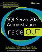
An index’s INCLUDE statement allows for data to be retrievable in the leaf level only, but not stored in the branch level. This reduces the overall size and complexity needed to cover a query’s need. Consider the following query and execution plan (see Figure 15-1) from the WideWorldImporters sample database. (Figure 15-2 shows the properties of the index seek in the following script.)
SELECT CustomerID, AccountsPersonID
FROM [Sales].[Invoices]
WHERE CustomerID = 832;
Figure 15-1 This execution plan shows an index seek and a key lookup on the same table. The Key Lookup represents 99 percent of the cost of the query.

Figure 15-2 The properties of the Index Seek in the previous sample script. Note that CustomerID is in the seek predicate and also in the output list, but that AccountsPersonID is not listed in the output list.
Note in Figure 15-2 that CustomerID is in the seek predicate and also in the output list, but that AccountsPersonID is not listed in the output list. Our query is searching for and returning CustomerID (it appears in both the SELECT and WHERE clauses), but our query also returns AccountsPersonID, which is not contained in the index FK_Sales_Invoices_CustomerID. (It searches the indexes then joins that result with the clustered index.)
Here is the code of the nonclustered index FK_Sales_Invoices_CustomerID, named because it is for CustomerID, a foreign key reference:
CREATE NONCLUSTERED INDEX [FK_Sales_Invoices_CustomerID]
ON [Sales].[Invoices]
( CustomerID ASC );
To remove the key lookup, add an included column to the nonclustered index so the query can retrieve all the data it needs from a single object:
CREATE NONCLUSTERED INDEX [FK_Sales_Invoices_CustomerID]
ON [Sales].[Invoices]
( CustomerID ASC )
INCLUDE ( AccountsPersonID )
WITH (DROP_EXISTING = ON);
GO
Let’s run our sample query again (see Figure 15-3):
SELECT CustomerID, AccountsPersonID
FROM [Sales].[Invoices]
WHERE CustomerID = 832;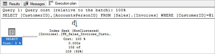
Figure 15-3 The execution plan now shows only an index seek. The key lookup that appeared in Figure 15-1 has been eliminated from the execution plan.
Note in Figure 15-3 that the key lookup has been eliminated. The query was able to retrieve both CustomerID and AccountsPersonID from the same index and required no second probe of the table for AccountsPersonID. The estimated subtree cost, in the properties of the SELECT operator, is now 0.0034015, compared to 0.355919 when the key lookup was present. Although this query was a small example for demonstration purposes, eliminating the key lookup represents a cost reduction by two orders of magnitude, without changing the query.
Just as you do not want to add too many nonclustered indexes, you also do not want to add too many columns unnecessarily to the INCLUDE list of nonclustered indexes. Columns in the INCLUDE list, as you saw in the previous code example, still require storage space. For infrequent queries that return small sets of data, the key lookup operator is probably not worth the cost of storing additional columns in the INCLUDE list of an index. Every time you include a column, you increase the overhead of the index.
In summary, you should craft nonclustered indexes to serve many queries intelligently, you should always try to avoid creating overlapping or redundant indexes, and you should regularly review to verify that indexes are still being used as applications or report queries change. Keep this guidance in mind as you move into the next section!
Create filtered nonclustered indexes
Nonclustered indexes are a sort of vertical partition of a table, but you can also create a horizontal filter of an index. A filtered index has powerful potential uses to serve up prefiltered data. Obviously, filtered indexes are only then suited to serve data to queries with matching WHERE clauses.
Filtered indexes could have particular use in table designs that include a soft delete flag, a processed/unprocessed status flag, or a current/archived flag. Work with developers to identify this sort of table design usage.
Imagine a scenario where a table has millions of rows, with a few rows marked as “unprocessed” and the rest marked as “processed.” An application might regularly query this table using WHERE processed = 0, looking for rows to process. A nonclustered index on the processed column, resulting in a seek operation in the execution plan, would be much faster than scanning the entire table. But a filtered index with the same WHERE clause would only contain the few rows marked “unprocessed,” resulting in a performance gain for the same query with no code changes.
You can easily add a filter to an index. For example:
CREATE INDEX [IX_Application_People_IsEmployee]
ON [Application].[People]([IsEmployee]) WHERE IsEmployee = 1
WITH (DROP_EXISTING = ON);
In your database, look for potential uses of new filtered indexes in columns that are of the bit data type, use a prefix like “Is” or a suffix like “Flag,” or perhaps, when a query only ever looks for data of a certain type, or data that is NULL or NOT NULL. Work with developers to identify potential uses when the majority of data in the table is not needed for many queries.
Adding a filter to an existing index might make it unusable to queries that do not use the same query. Avoid adding a filter to an existing nonclustered index marked unique, as this will change the enforcement of the constraint and the intent of the unique index. Filtered nonclustered indexes can be created with the unique property to enforce filtered uniqueness. For example, this could have potential uses in employee IDs that are allowed to be reused, or in a data warehouse scenario where a table needs to enforce uniqueness on only the active records of a dimension.
Understand the missing indexes feature
The concept of intelligently combining many similar indexes into one super-index is crucial to understanding the utility of using SQL Server’s built-in missing indexes feature. First introduced in SQL Server 2005, the missing indexes feature revolutionized the ability to see the big picture when crafting nonclustered indexes. The missing indexes feature has been passively gathering information on every database since SQL Server 2005 as well as in Azure SQL Database.
The missing indexes feature collects information from actual query usage. SQL Server passively records when it would have been better to have a nonclustered index—for example, to replace a scan for a seek, or to eliminate a lookup from a query’s execution plan. The missing indexes feature then aggregates these requests, counts how many times they have occurred, calculates the cost of the statement operations that could be improved, and estimates the percentage of that cost that would be eliminated (this percentage is labeled the impact). Think of the missing indexes feature as the database wish list of nonclustered indexes.
There are, however, some caveats and limitations with regard to the missing indexes feature. The recommendations in the output of the missing index dynamic management objects (DMOs) will likely include overlapping (but not duplicate) suggestions. Also, only rowstore nonclustered indexes can be suggested—remember this feature was introduced in SQL Server 2005—so clustered columnstore and other types of indexes won’t be recommended. Finally, recommendations are lost when any data definition language (DDL) changes to the table occur and when the SQL Server instance restarts.
You can look at missing indexes any time, with no performance overhead to the server, by querying a set of DMOs dedicated to this feature. You can find the following query, which concatenates the CREATE INDEX statement for you according to a simple, self-explanatory naming convention. As you can see from the use of system views, this query is intended to be run in a single database:
SELECT mid.[statement], create_index_statement =
      CONCAT('CREATE NONCLUSTERED INDEX IDX_NC_'
    , TRANSLATE(replace(mid.equality_columns, ' ' ,''), '],[' ,'___')
    , TRANSLATE(replace(mid.inequality_columns, ' ' ,''), '],[' ,'___')
    , ' ON ' , mid.[statement] , ' (' , mid.equality_columns
    , CASE WHEN mid.equality_columns IS NOT NULL
     AND mid.inequality_columns IS NOT NULL THEN ',' ELSE '' END
    , mid.inequality_columns , ')'
    , ' INCLUDE ('+ , mid.included_columns ,+ ')' )
, migs.unique_compiles, migs.user_seeks, migs.user_scans
, migs.last_user_seek, migs.avg_total_user_cost
, migs.avg_user_impact, mid.equality_columns
, mid.inequality_columns, mid.included_columns
FROM sys.dm_db_missing_index_groups mig
INNER JOIN sys.dm_db_missing_index_group_stats migs
ON migs.group_handle = mig.index_group_handle
INNER JOIN sys.dm_db_missing_index_details mid
ON mig.index_handle = mid.index_handle
INNER JOIN sys.tables t ON t.object_id = mid.object_id
INNER JOIN sys.schemas s ON s.schema_id = t.schema_id
WHERE mid.database_id = DB_ID()
-- count of query compilations that needed this proposed index
--AND       migs.unique_compiles > 10
-- count of query seeks that needed this proposed index
--AND       migs.user_seeks > 10
-- average percentage of cost that could be alleviated with this proposed index
--AND       migs.avg_user_impact > 75
-- Sort by indexes that will have the most impact to the costliest queries
ORDER BY migs.avg_user_impact * migs.avg_total_user_cost desc;
At the bottom of this query is a series of filters that you can use to find only the most-used, highest-value index suggestions. If this query returns hundreds or thousands of rows, consider spending an afternoon crafting together indexes to improve the performance of the actual user activity that generated this data.
Some indexes returned by the missing indexes queries might not be worth creating because they have a very low impact or have been part of only one query compilation. Others might overlap each other. For example, you might see these three index suggestions:
CREATE NONCLUSTERED INDEX IDX_NC_Gamelog_Team1 ON dbo.gamelog (Team1) INCLUDE (GameYear,
GameWeek, Team1Score, Team2Score);
CREATE NONCLUSTERED INDEX IDX_NC_Gamelog_Team1_GameWeek_GameYear ON dbo.gamelog (Team1,
GameWeek, GameYear) INCLUDE (Team1Score);
CREATE NONCLUSTERED INDEX IDX_NC_Gamelog_Team1_GameWeek_GameYear_Team2 ON dbo.gamelog
(Team1, GameWeek, GameYear, Team2);
You should not create all three of these indexes. Instead, you should combine the indexes you deem useful and worthwhile into a single index that matches the order of the needed key columns and covers all the included columns, as well. Here is the properly combined index suggestion:
CREATE NONCLUSTERED INDEX IDX_NC_Gamelog_Team1_GameWeek_GameYear_Team2
ON dbo.gamelog (Team1, GameWeek, GameYear, Team2)
INCLUDE (Team1Score, Team2Score);
This last index is a good combination of the previous suggestions. It delivers maximum positive benefit to the most queries and minimizes the negative impact to writes, storage, and maintenance. Note that the key columns list overlaps and is in the correct order for each of the previous index suggestions, and that the INCLUDE columns list also covers all the columns needed in the index suggestions. If a column is in the key of the index, it does not need to exist in the INCLUDE of the index.
However, don’t create this index yet. You should still review existing indexes on the table before creating any missing indexes. Perhaps you can combine a new missing index and an existing index, in the key column list or the INCLUDE column list, further increasing the value of a single index.
After combining missing index suggestions with each other and with existing indexes, you are ready to create the index and see it in action. Remember: Always look at the big picture when creating indexes. Rarely does a single query rise to the level of importance of justifying its own indexes. For example, in SSMS, you will sometimes see text suggesting a missing index for this query, as illustrated in Figure 15-4. (This text will be green on your screen, but appears gray in this book.)

Figure 15-4 In the Execution plan tab, in the header of each execution plan. Text starting with “Missing Index” will alert you to the possible impact. Do not create this index on the spot!
This is somewhat valuable, but do not create this index on the spot! Always refer to the complete set of index suggestions and other existing indexes on the table, combining overlapping indexes when possible. Consider the green missing index alert in SSMS as only a flag that indicates you should spend time investigating new missing indexes.
To recap, when creating nonclustered indexes for performance tuning, you should do the following:
Use the missing index DMVs to identify new big-picture nonclustered indexes:
Don’t create indexes that will likely only help out a single query; few queries are important enough to deserve their own indexes.
Consider nonclustered columnstore indexes for very large rowcount tables where queries often have to scan millions of rows for aggregates. (You can read more on columnstore indexes later in this chapter.)
Combine missing index suggestions, being aware of key order and
INCLUDElists.Compare new index suggestions with existing indexes; perhaps you can combine them.
Review index usage statistics to verify whether indexes are helping you. (More on the index usage statistics DMV in a moment.)
Understand when missing index suggestions are removed
Missing index suggestions are cleared out for any change to the tables—for example, if you add or remove columns or indexes. Missing index suggestions are also cleared out when the SQL Server service is started and cannot be manually cleared easily. (You can take the database offline and back online, which would clear out the missing index suggestions, but this seems like overkill.)
Logically, make sure the missing index data that you have collected is also based on a significant sample of actual production user activity over time spanning at least one business cycle. Missing index suggestions based on development activity might not be a useful representation of intended application activity, though suggestions based on end-user testing or training could be.
Understand and provide index usage
You’ve added indexes to your tables, and they are used over time, but meanwhile the query patterns of applications and reports change. Columns are added to the database, new tables are added, and although you add new indexes to suit new functionality, how does a database administrator ensure that existing indexes are still worth keeping?
SQL Server tracks this information for you automatically with yet another valuable DMV: sys.dm_db_index_usage_stats. Following is a script that measures index usage within a database, combining sys.dm_db_index_usage_stats with other system views and DMVs to return valuable information. Note that the ORDER BY clause places indexes with the fewest read operations (seeks, scans, lookups) and the most write operations (updates) at the top of the list.
SELECT TableName = sc.name + '.' + o.name, IndexName = i.name
     , s.user_seeks, s.user_scans, s.user_lookups
     , s.user_updates
     , ps.row_count, SizeMb = (ps.in_row_reserved_page_count*8.)/1024.
     , s.last_user_lookup, s.last_user_scan, s.last_user_seek
     , s.last_user_update
FROM sys.dm_db_index_usage_stats AS s
  INNER JOIN sys.indexes AS i
ON i.object_id = s.object_id AND i.index_id = s.index_id
   INNER JOIN sys.objects AS o ON o.object_id=i.object_id
   INNER JOIN sys.schemas AS sc ON sc.schema_id = o.schema_id
    INNER JOIN sys.partitions AS pr
ON pr.object_id = i.object_id AND pr.index_id = i.index_id
    INNER JOIN sys.dm_db_partition_stats AS ps
ON ps.object_id = i.object_id AND ps.partition_id = pr.partition_id
WHERE o.is_ms_shipped = 0
--Don't consider dropping any constraints
AND i.is_unique = 0 AND i.is_primary_key = 0 AND i.is_unique_constraint = 0
--Order by table reads asc, table writes desc
ORDER BY user_seeks + user_scans + user_lookups asc, s.user_updates desc;
Any indexes that rise to the top of the preceding query should be considered for removal or redesign, given the following caveats:
Before dropping any indexes, you should ensure you have collected data from the index usage stats DMV that spans at least one complete business cycle. The index usage stats DMV is cleared when the SQL Server service is restarted. You cannot manually clear it. If your applications have week-end and month-end reporting, you might have indexes present and tuned specifically for those critical performance periods.
Logically, verify that the index usage data that you have collected is based on actual production user activity. Index usage data based on testing or development activity would not be a useful representation of intended application activity.
Note the final
WHEREclause that ignores unique constraints and primary keys. Even if a nonclustered index exists and isn’t used, if it is part of the uniqueness of the table, it should not be dropped.
Again, the Query Store can be an invaluable tool to monitor for query regression after indexing changes.
- For more info on the Query Store, see Chapter 14.
Like many DMVs that are cleared when the SQL Server service restarts, consider a strategy of capturing data and storing index usage history periodically in persistent tables.
Server-scoped dynamic management views and functions require VIEW SERVER STATE permission on the server. Database-scoped dynamic management views and functions require VIEW DATABASE STATE permission on the database.
Understand columnstore indexes
Columnstore indexes were first introduced in SQL Server 2012, making a splash in their ability to far outperform clustered and nonclustered indexes for aggregations. They were typically used in the scenario of nightly refreshed data warehouses, but now they have beneficial applications on transactional systems, including on memory-optimized tables.
Since their introduction, the evolution of columnstore indexes has greatly expanded their usefulness:
Before SQL Server 2016, the presence of a nonclustered columnstore index made the table read-only. This drawback was removed in SQL Server 2016; now nonclustered columnstore indexes are fully featured and quite useful in a variety of applications aside from nightly refresh databases.
Starting with SQL Server 2016 with Service Pack 1, columnstore indexes became available below Enterprise edition licenses of SQL Server (though with a limitation on columnstore memory utilization).
Snapshot isolation and columnstore indexes are fully compatible. Before SQL Server 2016, using read-committed snapshots and snapshot isolation levels was not supported with columnstore indexes.
You can place a clustered columnstore index on a memory-optimized table, providing the ability to do analytics on millions of rows of live real-time online transactional processing (OLTP) data.
Starting with SQL Server 2017, a variety of batch mode features grouped under the intelligent query processing (IQP) label increased performance of queries with columnstore indexes.
- For more about the suite of features under IQP, see Chapter 14.
Starting with SQL Server 2019, using the
WITH (ONLINE = ON)syntax is supported for creating and rebuilding columnstore indexes.
These key improvements opened columnstore indexes to be used in transactional systems, when tables with millions of rows are read, resulting in million-row result sets.
Columnstore indexes have two compression levels. In addition to the eponymous default COLUMNSTORE compression level, there is also a COLUMNSTORE_ARCHIVE compression option, which further compresses the data at the cost of more CPU when needing to read or write the data.
As with rowstore indexes, you can compress each partition of a table’s columnstore index differently. Consider applying COLUMNSTORE_ARCHIVE compression to partitions of data that are old and rarely accessed. You can change the data compression option for rowstore and columnstore indexes by using the index rebuild operation via the DATA_COMPRESSION option. For columnstore indexes, you can specify the COLUMNSTORE or COLUMNSTORE_ARCHIVE options, whereas for rowstore indexes, you can use the NONE, ROW, and PAGE compression options.
- For more detail on data compression, see Chapter 3, “Design and implement an on-premises database infrastructure.”
You cannot change the compression option of a rowstore index to either of the columnstore options, or vice versa. Instead, you must build a new index of the desired type.
The sp_estimate_data_compression_savings system stored procedure can be used to estimate the size differences between the compression options. Starting with SQL Server 2019, this stored procedure includes estimates for the two columnstore compression options. In SQL Server 2022, sp_estimate_data_compression_savings can be used to estimate savings for XML compression as well.
- See the “XML compression” section at the end of the chapter for more information.
Note
There is currently a three-way incompatibility between the sp_estimate_data_compression_savings system stored procedure, columnstore indexes, and the memory-optimized tempdb metadata feature introduced in SQL Server 2019. You cannot use sp_estimate_data_compression_savings with columnstore indexes if the memory-optimized tempdb metadata feature is enabled. For more information visit https://learn.microsoft.com/sql/relational-databases/system-stored-procedures/sp-estimate-data-compression-savings-transact-sql.
Design columnstore indexes
Columnstore indexes don’t use a B+ tree; instead, they contain highly compressed data (on disk and in memory), stored in a different architecture from the traditional clustered and nonclustered indexes. They are the standard for storing and querying large data warehouse fact tables. Unlike rowstore indexes, there is no “key” or “include” of a columnstore index, only a set of columns that are part of the index. For non-ordered columnstore indexes, the order of the columns in the definition of index does not matter. This is the default index. You can create “clustered” or “nonclustered” columnstore indexes, though this terminology is used more to indicate what role the columnstore index is serving, not what it resembles behind the scenes.
Clustered columnstore indexes do not change the physical structure of the table like rowstore clustered indexes. Ordered clustered columnstore indexes sort the existing data in memory by the order key(s) before the index builder compresses them into index segments. Any sorted data overlap is reduced, which allows for better data elimination when querying, and therefore faster performance because the amount of data read from disk is smaller. If all data can be sorted in memory at once, then data overlap can be avoided. Owing to the size of tables in data warehouses, this scenario doesn’t happen often.
- For more information, visit https://learn.microsoft.com/azure/synapse-analytics/sql-data-warehouse/performance-tuning-ordered-cci.
You can also create nonclustered rowstore indexes on tables with a clustered columnstore index, which is potentially useful to enforce uniqueness, and support single row fetching, deleting, and updating. Columnstore indexes cannot be unique, and so cannot replace the table’s unique constraint or primary key. Clustered columnstore indexes might also perform poorly when a table receives updates, so consider the workload for a table before adding a clustered columnstore. Tables that are only ever inserted into, but never updated or deleted from, would be an ideal candidate for a clustered columnstore index.
You can combine nonclustered rowstore and nonclustered columnstore indexes on the same table, but you can have only one columnstore index on a table, including clustered and nonclustered columnstore indexes. You can even create nonclustered rowstore and nonclustered columnstore indexes on the same columns. Perhaps you create both because you want to filter on the column value in one set of queries, and aggregate in another. Or perhaps you create both only temporarily, for comparison.
You can also create nonclustered columnstore indexes on indexed views—another avenue to quick-updating analytical data. The stipulations and limitations regarding indexed views apply, but you would create a unique rowstore clustered index on the view, then a nonclustered columnstore view.
You can add columns in any order to satisfy many different queries, greatly increasing the versatility of the columnstore index in your table. This is because the order of the data is not important to how columnstore indexes work.
The size of the key for columnstore indexes, however, could make a big difference in performance. The columns in a columnstore index should each be limited to 8,000 bytes for best performance. Data larger than 8,000 bytes in a row is compressed separately outside of the columnstore compressed row group, requiring more decompression to access the complete row.
While the large object data types varchar(max), nvarchar(max), and varbinary(max) are supported in the key of a columnstore index, they are not stored in-line with the rest of the compressed data, but rather outside the columnstore structure. These data types are not recommended in columnstore indexes. Starting with SQL Server 2017, they are supported, but still not recommended.
- For more on data type restrictions and limitations for columnstore indexes, visit https://learn.microsoft.com/sql/t-sql/statements/create-columnstore-index-transact-sql#LimitRest.
The most optimal data types for columns in a columnstore index are data types that can be stored in an 8-byte integer value, such as integers and some date- and time-based data types. They allow you to use what is known as segment elimination. If your query includes a filter on such values, SQL Server can issue reads to only those segments in row groups that contain data within a range, eliminating ranges of data outside of the request. The data is not sorted, so segment elimination might not help all filtering queries, but the more selective the value, the more likely it will be useful. Other data types with a size less than 8,000 bytes will still compress and be useful for aggregations, but should generally not appear as a filter, because the entire table will always need to be scanned unless you add a nonclustered index.
Understand batch mode
Batch mode is one of the existing features lumped into the intelligent query processing (IQP) umbrella—a collection of performance improvements. Batch mode has actually been around since SQL Server 2014. Like many other features listed under IQP, batch mode can benefit workloads automatically and without requiring code changes.
Batch mode is useful in the following scenarios:
Analytical queries. Usually, these queries use operators like joins or aggregates that process hundreds of thousands of rows or more.
Your workload is CPU bound. However, you should consider a columnstore index even if your workload is I/O bound.
Heavy OLTP workload. You may decide that creating a columnstore index adds too much overhead to your heavy transactional workload, and your analytical workload is not as important.
Support. Your application depends on a feature that columnstore indexes don’t yet support.
Batch mode uses heuristics to determine whether it can move data into memory to be processed in a batch rather than row by row. Columnstore indexes reduce I/O and batch processing reduces CPU usage, ultimately speeding up the query.
You’ll see Batch (instead of the default Row) in the Actual Execution Mode of an execution plan operator when this faster method is in use. Batch mode processing appears in the form of batch mode operators in execution plans, and benefits queries that process millions of rows or more.
- For more information on IQP features, see Chapter 14.
Initially, only queries on columnstore indexes could benefit from batch mode operators. Starting with compatibility level 150 (SQL Server 2019), however, batch mode for analytic workloads became available outside of columnstore indexes. The query processor might decide to use batch mode operators for queries on heaps and rowstore indexes. No changes are needed for your code to benefit from batch mode on rowstore objects, as long as you are in compatibility level 150 or higher.
- For more information on which operators can use batch mode execution, go to https://learn.microsoft.com/sql/relational-databases/indexes/columnstore-indexes-query-performance.
Note
Batch mode has not yet been extended to in-memory OLTP tables or other types of indexes like full-text, spatial, or XML indexes. Batch mode will also not occur on sparse and XML columns.
Understand the deltastore of columnstore indexes
The columnstore deltastore is an ephemeral location where changed data is stored in a clustered B+ tree rowstore format. When certain thresholds of inserted rows are reached, typically 1,048,576 rows, or when a columnstore index is rebuilt or reorganized, a group of deltastore data is “closed.” Then, via a background thread called the tuple mover, the deltastore rowgroup is compressed into the columnstore. The number of rows SQL Server compresses into a rowgroup might be smaller under memory pressure, which happens dynamically.
The COMPRESSION_DELAY option for both nonclustered and clustered columnstore indexes has to do with how long it takes changed data to be written from the deltastore to the highly compressed columnstore.
The COMPRESSION_DELAY option does not affect the 1,048,576 number, but rather how long it takes SQL Server to move the data into the columnstore. If you set the COMPRESSION_DELAY option to 10 minutes, data will remain in the deltastore for at least an extra 10 minutes before SQL Server compresses it. The advantage of data remaining in the deltastore, delaying its eventual compression, could be noticeable on tables that continue to be updated and deleted. Updates and deletes are typically very resource intensive on columnstore indexes. Delete operations in the columnstore are “soft” deleted, marked as removed, and then eventually cleaned out during index maintenance. Updates are actually processed as deletes and inserts into the deltastore.
The advantage of COMPRESSION_DELAY is noticeable for some write workloads, but not all. If the table is only ever inserted into, COMPRESSION_DELAY doesn’t really help. But if a block of recent data is updated and deleted for a period before finally settling in after a time, implementing COMPRESSION_DELAY can speed up the write transactions to the data and reduce the maintenance and storage footprint of the columnstore index.
Changing the COMPRESSION_DELAY setting of the index, unlike many other index settings, does not require a rebuild of the index, and you can change it at any time. For example:
ALTER INDEX [NCCX_Sales_InvoiceLines]
    ON [Sales].[InvoiceLines]
    SET (COMPRESSION_DELAY = 10 MINUTES);
SQL Server can ignore the deltastore for inserts when you insert data in large amounts. This is called bulk loading in Microsoft documentation, but is not related to the BULK INSERT command. When you want to insert large amounts of data into a table with a columnstore index, SQL Server bypasses the deltastore. This increases the speed of the insert and the immediate availability for the data for analytical queries, and reduces the amount of logged activity in the user database transaction log.
Under ideal circumstances, the best number of rows to insert in a single statement is 1,048,576, which creates a complete, compressed columnstore row group. The number of rows to trigger a bulk load is between 102,400 rows and 1,047,576 rows, depending on memory. If you specify TABLOCK in the INSERT statement, bulk loading data into the columnstore occurs in parallel. The typical caveat about TABLOCK is applicable here, as the table might block other operations at the time of the insert in parallel.
Demonstrate the power of columnstore indexes
To demonstrate the power of this fully operational columnstore index, let’s review a scenario in which more than 14 million rows are added to the WideWorldImporters.Sales.InvoiceLines table. About half of the rows in the table now contain InvoiceID = 69776.
To demonstrate, start by restoring a fresh copy of the sample WideWorldImporters database from https://learn.microsoft.com/sql/samples/wide-world-importers-oltp-install-configure.
The following sample script drops the existing WideWorldImporters-provided nonclustered columnstore index and adds a new nonclustered index we’ve created here. This performs an index scan to return the data. Remember that InvoiceID = 69776 is roughly half the table, so this isn’t a “needle in a haystack” situation; it isn’t a seek. If the query can use a seek operator, the nonclustered rowstore index would likely be better. When the query must scan, columnstore is king.
USE WideWorldImporters;
GO
-- Fill haystack with 3+ million rows
INSERT INTO Sales.InvoiceLines (InvoiceLineID, InvoiceID
, StockItemID, Description, PackageTypeID, Quantity
, UnitPrice, TaxRate, TaxAmount, LineProfit, ExtendedPrice
, LastEditedBy, LastEditedWhen)
SELECT InvoiceLineID = NEXT VALUE FOR [Sequences].[InvoiceLineID]
, InvoiceID, StockItemID, Description, PackageTypeID, Quantity
, UnitPrice, TaxRate, TaxAmount, LineProfit
, ExtendedPrice, LastEditedBy, LastEditedWhen
FROM Sales.InvoiceLines;
GO 3 --Runs the above three times
-- Insert millions of records for InvoiceID 69776
INSERT INTO Sales.InvoiceLines (InvoiceLineID, InvoiceID
, StockItemID, Description, PackageTypeID, Quantity
, UnitPrice, TaxRate, TaxAmount, LineProfit, ExtendedPrice
, LastEditedBy, LastEditedWhen)
SELECT InvoiceLineID = NEXT VALUE FOR [Sequences].[InvoiceLineID]
, 69776, StockItemID, Description, PackageTypeID, Quantity
, UnitPrice, TaxRate, TaxAmount, LineProfit
, ExtendedPrice, LastEditedBy, LastEditedWhen
FROM Sales.InvoiceLines;
GO
--Clear cache, drop other indexes to only test our comparison scenario
DBCC FREEPROCCACHE
DROP INDEX IF EXISTS [NCCX_Sales_InvoiceLines]
ON [Sales].[InvoiceLines];
DROP INDEX IF EXISTS IDX_NC_InvoiceLines_InvoiceID_StockItemID_Quantity
ON [Sales].[InvoiceLines];
DROP INDEX IF EXISTS IDX_CS_InvoiceLines_InvoiceID_StockItemID_Quantity
ON [Sales].[InvoiceLines];
GO
--Create a rowstore nonclustered index for comparison
CREATE INDEX IDX_NC_InvoiceLines_InvoiceID_StockItemID_Quantity
     ON [Sales].[InvoiceLines] (InvoiceID, StockItemID, Quantity);
GO
Now that the data is loaded, you can perform the query again for testing. (See Figure 15-5.) Note we are using the STATISTICS TIME option to measure both CPU and total duration. (Remember to enable the actual query plan before executing the query.)
SET STATISTICS TIME ON;
SELECT il.StockItemID, AvgQuantity = AVG(il.quantity)
FROM [Sales].[InvoiceLines] AS il
WHERE il.InvoiceID = 69776 --1.8 million records
GROUP BY il.StockItemID;
SET STATISTICS TIME OFF;
Figure 15-5 The execution plan of our sample query starts with an Index Seek (NonClustered) on the rowstore nonclustered index. Note the large amount of parallelism operators along the way.
The sample query on 69776 had to work through 1.8 million records and returned 227 rows. With the rowstore nonclustered index, the cost of the query is 4.52 and completes in 844 ms of CPU time (due to parallelism), 194 ms of total time. (These durations will vary from system to system; the lab environment was a four-core Intel processor with Hyper-Threading enabled.)
Now, let’s create a columnstore index, and watch our analytical-scale query benefit.
Note
Starting with SQL Server 2019, using the WITH (ONLINE = ON) syntax is supported for creating and rebuilding columnstore indexes.
--Create a columnstore nonclustered index for comparison
CREATE COLUMNSTORE INDEX IDX_CS_InvoiceLines_InvoiceID_StockItemID_quantity
    ON [Sales].[InvoiceLines] (InvoiceID, StockItemID, Quantity) WITH (ONLINE = ON);
GO
Perform the query again for testing. Note again we are using the STATISTICS TIME option to measure both CPU and total duration. (See Figure 15-6.)
SET STATISTICS TIME ON;
--Run the same query as above, but now it will use the columnstore
SELECT il.StockItemID, AvgQuantity = AVG(il.quantity)
FROM [Sales].[InvoiceLines] AS il
WHERE il.InvoiceID = 69776 --1.8 million records
GROUP BY il.StockItemID;
SET STATISTICS TIME OFF;
Figure 15-6 The execution plan of our sample query, now starting with a Columnstore Index Scan (NonClustered).
The sample query on 69776 still returns 227 rows. With the benefit of the columnstore nonclustered index, however, the cost of the query is 1.54 and completes in 47 ms of CPU time, 160 ms of total time. This is a significant but relatively small sample of the power of a columnstore index on analytical scale queries.
Understand indexes in memory-optimized tables
Memory-optimized tables support table performance less bound by I/O constraints, providing high-performance, latchless writes. Memory-optimized tables don’t use the locking mechanics of pessimistic concurrency, as discussed in Chapter 14. Data rows for memory-optimized tables are not stored in data pages, and so do not use the concepts of disk-based tables.
Memory-optimized tables can have two types of indexes: hash and nonclustered. Nonclustered indexes for memory-optimized tables behave similarly on memory-optimized tables as they do for disk-based tables, whereas hash indexes are better suited for high-performance seeks for individual records. You must create at least one index on a memory-optimized table. Either of the two types of indexes can be the structure behind the primary key of the table, if you want both the data and the schema to be durable.
Indexes on in-memory tables are never durable and will be rebuilt whenever the database comes online. The schema of the memory-optimized table is always durable; however, you can choose to have only the schema of the table be durable, not the data. This has utility in certain scenarios as a staging table to receive data that will be moved to a durable disk-based or memory-optimized table. You should be aware of the potential for data loss. If only the schema of the memory-optimized table is durable, you do not need to declare a primary key. However, in the CREATE TABLE statement, you must still define at least one index or a primary key for a table by using DURABILITY = SCHEMA_ONLY. Our suggestion is that only in very rare situations should a table not have a primary key constraint, no matter the durability.
Adding indexes to memory-optimized tables increases the amount of server memory needed. There is otherwise no limit to the size of memory-optimized tables in Enterprise edition; however, in Standard edition, you are limited to 32 GB of memory-optimized tables per database.
Earlier versions of SQL Server put a cap on the number of indexes on a memory-optimized table. That cap was raised from 8 to 999 in SQL Server 2017.
Although there is no concept of a rowstore clustered index in memory-optimized tables, you can add a clustered columnstore index to a memory-optimized table, dramatically improving your ability to perform analytical scale queries on the data even as it is rapidly inserted. Because columnstore indexes cannot be unique, they cannot serve as the primary key for a memory-optimized table.
Let’s go over the basics of using hash and nonclustered indexes on memory-optimized tables.
Understand hash indexes for memory-optimized tables
Memory-optimized hash indexes are an alternative to the typical B+ tree internal architecture for index data storage. Hash indexes are best for queries that look for the needle in the haystack, and are especially effective when matching exact values, but they are not effective at range lookups or queries with an ORDER BY.
One other limitation of the hash index is that if you don’t query all the columns in a hash index, they are generally not useful. The WHERE clause must try to seek each column in the hash index’s key. When there are multiple columns in the key of the indexes but not all columns—or even just the first column—are queried, hash indexes do not perform well. This is different from B+ tree-based nonclustered indexes, which perform fine if only the first column of the index’s key is queried.
Hash indexes are currently available only for memory-optimized tables, not disk-based tables. You can declare them by using the UNIQUE keyword, but they default to a non-unique key. You can create more than one hash index.
There is an additional unique consideration for creating hash indexes. Estimating the best number for the BUCKET_COUNT parameter can have a significant impact. The number should be as close as possible to the number of unique key values that are expected. BUCKET_COUNT should be between 1 and 2 times this number.
Hash indexes always use the same amount of space for the same-sized bucket count, regardless of the rowcount within. For example, if you expect the table to have 100,000 unique values in it, the ideal BUCKET_COUNT value would be between 100,000 and 200,000.
Having too many or too few buckets in a hash index can result in poor performance. More buckets will increase the amount of memory needed and the number of those buckets that are empty. Too few buckets will result in queries needing to access more, larger buckets in a chain to access the same information.
Ideally, a hash index is declared unique. Hash indexes work best when the key values are unique or at least highly distinct. If the ratio of total rows to unique key values is too high, a hash index is not recommended and will perform poorly. Microsoft recommends a threshold of less than 10 rows per unique value for an effective hash index. If you have data with many duplicate values, consider a nonclustered index instead.
You should periodically and proactively compare the number of unique key values to the total number of rows in the table. It is better to overestimate the number of buckets. You can change the number of buckets in a memory-optimized hash index by using the ALTER TABLE/ALTER INDEX/REBUILD commands. For example:
ALTER TABLE [dbo].[Transactions]
ALTER INDEX [IDX_NC_H Transactions_1]
REBUILD WITH (BUCKET_COUNT = 524288);
--will always round up to the nearest power of two
Understand nonclustered indexes for memory-optimized tables
Nonclustered indexes for memory-optimized tables behave similarly on memory-optimized tables to how they behave on disk-based tables. Instead of a B+ tree like a rowstore, disk-based nonclustered index, they are in fact a variant of the B-tree structure called the Bw-tree, which does not use locks or latches. They outperform hash indexes for queries that perform sorting on the key value(s) of the index, or when the index must be range scanned. Further, if you don’t query all the columns in a hash index, they are generally not as useful as a nonclustered index.
You can declare nonclustered indexes on memory-optimized tables unique. However, the CREATE INDEX syntax is not supported. You must use the ALTER TABLE/ADD INDEX commands or include them in the CREATE TABLE script.
Neither hash indexes nor nonclustered indexes can serve queries on memory-optimized tables for which the keys are sorted in the reverse order from how they are defined in the index. These types of queries simply can’t currently be serviced efficiently from memory-optimized indexes. If you need another sort order, you need to add the same B-tree index with a different sort order.
Remember: You can also add a clustered columnstore index to a memory-optimized table, dramatically improving your ability to analyze fast-changing data.
Understand index statistics
When we talk about statistics in SQL Server, we do not mean the term generically. Statistics on one or more columns in tables and views are created as needed by the Query Optimizer to describe the distribution of data within indexes and heaps.
Statistics are important to the Query Optimizer to help it make query plan decisions, and they are heavily involved in the concept of cardinality estimation. The SQL Server cardinality estimator (CE) provides accurate estimations of the number of rows that queries will return—a big part of producing query plans.
- For more on the performance impact of statistics on cardinality estimation, see Chapter 14.
Making sure statistics are available and up to date is essential for choosing a well-performing query plan. Stale statistics that have evaded updates for too long contain information that is quite different from the current state of the table and will likely cause poor execution plans.
There are several options in each database regarding statistics maintenance. Chapter 4, “Install and configure SQL Server instances and features,” reviews some of these, but we present them again here in the context of understanding how indexes are used for performance tuning.
Automatically create and update statistics
Most statistics needed for describing data to the SQL Server are created automatically, because the AUTO_CREATE_STATISTICS database option is enabled by default. This results in automatically created indexes with the _WA_Sys_<column_name>_<object_id_hex> naming convention.
When the AUTO_CREATE_STATISTICS database option is enabled, SQL Server can create single-column statistics objects based on query need. These can make a big difference in performance. You can determine that a statistics object was created by the AUTO_CREATE_STATISTICS = ON behavior because it will have the name prefix _WA. You can also use the following query:
SELECT *
FROM sys.stats
WHERE auto_created = 1;
The behavior that creates statistics for indexes (with a matching name) happens automatically, regardless of the AUTO_CREATE_STATISTICS database option.
Statistics are not automatically created for columnstore indexes. Instead, statistics objects that exist on the heap or the clustered index of the table are used. As with any index, a statistics object of the same name is created; however, for columnstore indexes it is blank, and in place for logistical reasons only. This statistics object is actually populated on the fly and not persisted in storage.
As you can imagine, statistics must also be kept up to date with the data in the table. SQL Server has an option in each database for AUTO_UPDATE_STATISTICS, which is ON by default and should almost always remain on.
You should only ever disable both AUTO_CREATE_STATISTICS and AUTO_UPDATE_STATISTICS when requested by highly complex application designs, with variable schema usage, and a separate regular process that creates and maintains statistics, such as Microsoft SharePoint. On-premises SharePoint installations include a set of stored procedures that periodically run to create and update the statistics objects for the wide, dynamically assigned table structures within. If you have not designed your application to intelligently create and update statistics using a separate process from that of the SQL Server engine, we recommend that you never disable these options.
Manually create statistics for on-disk tables
You can also create statistics manually during troubleshooting or performance tuning by using the CREATE STATISTICS statement.
Consider manually creating statistics for large tables, and with design principles similar to how nonclustered indexes should be created. The order of the keys in statistics does matter, and you should choose columns that are regularly queried together to provide the most value to queries.
When venturing into creating your own statistics objects, consider using filtered statistics, which can also be helpful if you are trying to carry out advanced performance tuning on queries with a static filter or specific range of data. Like filtered indexes (covered earlier in this chapter) or even filtered views and queries, you can create statistics with a similar WHERE clause. Filtered statistics are never automatically created.
- For more information on maintaining index statistics, see Chapter 8.
Understand statistics on memory-optimized tables
Statistics are created and updated automatically on memory-optimized tables, and serve the same role as they do for on-disk structures. Memory-optimized tables require at least one index to be created, and a matching statistics object is created for that index object.
It is recommended to always create memory-optimized tables in databases with the highest compatibility level. If a memory-optimized table was created with a SQL Server 2014 (12.0) compatibility level, you must manually update the statistics object using the UPDATE STATISTICS command. Then, if the AUTO_UPDATE_STATISTICS database option is enabled, statistics will update as normal. Statistics for new memory-optimized tables are not automatically updated if the database compatibility level was below compatibility level 130 when the tables were created.
- For more on memory-optimized tables, see Chapter 7, “Understand table features.”
Understand statistics on external tables
You can also create statistics on external tables—that is, tables that do not exist in the SQL Server database but instead are transparent references to data stored in Azure Blob Storage via PolyBase.
You can create statistics on external tables, but currently, you cannot update them. Creating the statistics object involves copying the external data into the SQL Server database only temporarily, and then calculating statistics. To update statistics for these datasets, you must drop them and re-create the statistics. Because of the data sizes typically involved with external tables, using the FULLSCAN method to update statistics is not recommended.
- For more on external tables, see Chapter 7.
Understand other types of indexes
There are other types of indexes that you should be aware of, each with specific, limited uses for certain SQL Server features—for example, the Full-Text Search engine, spatial data types, and the xml data type. Though not nearly as common as other types of indexes mentioned in this chapter, they have powerful specific uses.
Understand full-text indexes
If you have chosen to install the SQL Server Full-Text Search feature, you can take advantage of the full-text service (fdhost.exe) to query vast amounts of data using special full-text syntax, looking for word forms, phrases, thesaurus lookups, word proximity, and more. (You can of course choose to add the feature via SQL Server Setup if it is not already installed.)
Because they have specific uses for particular architectures and applications, we won’t spend much time on them here. Developers might take advantage of powerful full-text functions CONTAINS or FREETEXT.
By design, full-text indexes require a unique nonclustered or clustered rowstore index on the table in which they are created, with a single column in the key. We recommend that you give this index an integer key for performance reasons, such as an identity column. Full-text indexes are usually placed on varchar or nvarchar columns, often with large lengths, but you can also place them on xml and varbinary columns.
It is important to understand the two viable options to updating the full-text index. A full population of the full-text index is effective but will consume more resources than an incremental load strategy. If the table receives writes frequently, you should consider the two possible incremental load strategies. By default, the CHANGE_TRACKING AUTO option enables the change tracking feature on the table that hosts the full-text index, which makes it possible for changes to propagate into the full-text index. This asynchronously keeps the full-text data synchronized with minimal overhead. If enabling change tracking is not an option for the table, you can instead add or use an existing column with the timestamp data type in the table and then periodically update the full-text index by starting an incremental population. Consider both strategies, along with your requirements for frequency of updates to the full-text index. Both are superior to frequent full populations.
Understand spatial indexes
A spatial index is a special B-tree index that uses a suite of special code and geometry methods to assist in performing spatial and geometry calculations. Developers can use these data structures for non-Euclidean geometry calculations, distance and area calculations on spheres, and more. Spatial indexes can improve the performance of queries with spatial operations.
You can create these indexes only on columns that use the spatial data types geometry or geography, and you can create different types of indexes on the same spatial column to serve different calculations. To create a spatial index, the table must already have a primary key.
You create spatial indexes by using bounding boxes or tessellation schemes for geometry and geography data types. Consult the documentation and the developers’ intended use of spatial data when creating these indexes here: https://learn.microsoft.com/sql/relational-databases/spatial/spatial-indexes-overview.
Understand XML indexes
XML indexes are created for much the same benefit as nonclustered indexes. You use them to prevent the runtime shredding of XML files each time they are accessed, and to instead provide a persistent row set of the XML data’s tags, values, and paths.
Because the xml data type is stored as a BLOB and has an upper limit of 2 GB of data per row, XML data can be massive, and XML indexes can be extremely beneficial to reads. Like nonclustered indexes, they also incur an overhead to writes.
Primary XML indexes prevent the on-demand shredding of the data by providing a reference to the tags, values, and paths. On large XML documents, this can be a major performance improvement.
Secondary XML indexes enhance the performance of primary XML indexes. They are created on either path, value, or property data in the primary XML index and benefit a read workload that heavily uses one of those three methods of querying XML data.
- Consult the documentation and the developers’ intended use of XML data when creating XML indexes at https://learn.microsoft.com/sql/relational-databases/xml/xml-indexes-sql-server.
XML compression
SQL Server 2022 introduces XML compression, which can compress off-row XML data for both XML columns and XML indexes, providing a much-needed improvement when storing XML data in SQL Server.
When you enable XML compression, the underlying storage is changed to a compressed binary format, but this doesn’t change how you query the data, and it doesn’t require any application changes.
Although XML compression works in a similar way to data compression, it only affects the xml data type and associated XML indexes. You can run data compression and XML compression side by side on the same tables, but it must be enabled explicitly on primary and secondary XML indexes.
Space saving with XML compression
The similarity with data compression extends to two system objects: the sp_estimate_data_compression_savings system stored procedure and the sys.dm_db_index_physical_stats dynamic management function.
You can use sp_estimate_data_compression_savings to estimate how much space you will save by compressing XML columns and indexes. In SQL Server 2022, this stored procedure takes a new parameter, @xml_compression, which is a Boolean value. You can assign it a bit value of 1, 0, or NULL (the default).
To find out how much space you have saved once you have compressed your XML data, use sys.dm_db_index-physical_stats. The following query returns the average row size in bytes, number of records, and number of data pages occupied to show you the benefits of compression:
SELECT o.name,
    ips.partition_number,
    ips.index_type_desc,
    ips.record_count, ips.avg_record_size_in_bytes,
    ips.min_record_size_in_bytes,
    ips.max_record_size_in_bytes,
    ips.page_count, ips.compressed_page_count
FROM sys.dm_db_index_physical_stats ( DB_ID(), NULL, NULL, NULL, 'DETAILED') ips
JOIN sys.objects o on o.object_id = ips.object_id
ORDER BY record_count DESC;