
Chapter 5
R1C1-style formulas
In this chapter, you will:
Understand A1 versus R1C1 references
Toggle to R1C1-style references
Witness the miracle of Excel formulas
Examine the R1C1 reference style
Understanding R1C1 formulas will make your job easier in VBA. You could skip this chapter, but if you do, your code will be harder to write. Taking 30 minutes to understand R1C1 will make every macro you write for the rest of your life easier to code.
We can trace the A1 style of referencing back to VisiCalc. Dan Bricklin and Bob Frankston used A1 to refer to the cell in the upper-left corner of the spreadsheet. Mitch Kapor used this same addressing scheme in Lotus 1-2-3. Upstart Multiplan from Microsoft attempted to buck the trend and used something called R1C1-style addressing. In R1C1 addressing, the cell known as A1 is referred to as R1C1 because it is in row 1, column 1.
With the dominance of Lotus 1-2-3 in the 1980s and early 1990s, the A1 style became the standard. Microsoft realized it was fighting a losing battle and eventually offered either R1C1-style addressing or A1-style addressing in Excel. When you open Excel today, the A1 style is used by default. Officially, however, Microsoft supports both styles of addressing.
You would think that this chapter would be a non-issue. Anyone who uses the Excel interface would agree that the R1C1 style is dead. However, we have what on the face of it seems to be an annoying problem: The macro recorder records formulas in the R1C1 style. So you might be thinking that you just need to learn R1C1 addressing so that you can read the recorded code and switch it back to the familiar A1 style.
I have to give Microsoft credit. R1C1-style formulas, you’ll grow to understand, are actually more efficient, especially when you are dealing with writing formulas in VBA. Using R1C1-style addressing enables you to write more efficient code.
Toggling to R1C1-style references
You don’t need to switch to R1C1 style in order to use .FormulaR1C1 in your code. However, while you’re learning about R1C1, it helps to temporarily switch to R1C1 style.
To switch to R1C1-style addressing, select Options from the File menu. In the Formulas category, select the R1C1 Reference Style check box (see Figure 5-1).
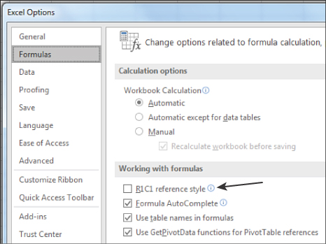
FIGURE 5-1 Selecting the R1C1 reference style in the Formulas category of the Excel Options dialog box causes Excel to use R1C1 style in the Excel user interface.
After you switch to R1C1 style, the column letters A, B, C, D across the top of the worksheet are replaced by the numbers 1, 2, 3, 4 (see Figure 5-2).
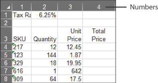
FIGURE 5-2 In R1C1 style, the column letters are replaced by numbers.
In this format, the cell that you know as B5 is called R5C2 because it is in row 5, column 2.
Every couple of weeks, someone manages to accidentally turn on this option, and we get an urgent support request at MrExcel. This style is foreign to 99% of spreadsheet users.
Witnessing the miracle of Excel formulas
Automatically recalculating thousands of cells is the main benefit of electronic spreadsheets over the green ledger paper used up until 1979. However, a close second-prize award would be that you can enter one formula and copy that formula to thousands of cells.
Entering a formula once and copying 1,000 times
Switch back to A1 style referencing. Consider the worksheet shown in Figure 5-3. Enter a simple formula such as =B4*C4 in cell D4, double-click the AutoFill handle, and the formula intelligently changes as it is copied down the range.
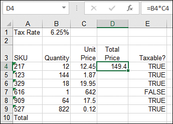
FIGURE 5-3 Double-click the AutoFill handle, and Excel intelligently copies this relative-reference formula down the column.
The formula is rewritten for each row, eventually becoming =C9*B9. It seems intimidating to consider having a macro enter all these different formulas. Figure 5-4 shows how the formulas change when you copy them down columns D, F, and G.
![]() Note
Note
Press Ctrl+’ to switch to showing formulas rather than their results. Press it again to toggle back to seeing values.
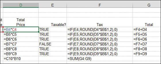
FIGURE 5-4 Amazingly, Excel adjusts the cell references in each formula as you copy down the column.
The formula in cell F4 includes both relative and absolute formulas: =IF(E4,ROUND(D4*$B$1,2),0). Thanks to the dollar signs inserted in cell B1, you can copy down this formula, and it always multiplies the total price in this row by the tax rate in cell B1.
The secret: It’s not that amazing
Excel actually uses R1C1-style formulas behind the scenes. Excel shows addresses and formulas in A1 style merely because it needs to adhere to the standard made popular by VisiCalc and Lotus.
If you switch the worksheet in Figure 5-4 to use R1C1 notation, you can see that the “different” formulas in D4:D9 are all actually identical formulas in R1C1 notation. The same is true of F4:F9 and G4:G9.
Use the Options dialog box to change the sample worksheet to R1C1-style addresses. If you examine the formulas in Figure 5-5, you see that in R1C1 language, every formula in column 4 is identical. Given that Excel is storing the formulas in R1C1 style, copying them, and then merely translating to A1 style for us to understand, it is no longer that amazing that Excel can manipulate A1-style formulas as easily as it does.
![This figure repeats the view from Figure 5-4, but the worksheet is in R1C1 Formula mode. In this mode, every formula in column 4 is identical: =RC[-2]*RC[-1]. Even in column F, the formula with absolute references is identical all the way down the column: =IF(RC[-1],ROUND(RC[-2]*R1C2,2),0).](https://imgdetail.ebookreading.net/2023/10/9780137521531/9780137521531__9780137521531__files__graphics__05fig05.jpg)
FIGURE 5-5 The same formulas as in Figure 5-4 are shown in R1C1 style. Note that every formula in column 4 is the same, and every formula in column 6 is the same.
This is one of the reasons R1C1-style formulas are more efficient than A1-style formulas in VBA. When you have the same formula being entered in an entire range, it is less confusing.
![]() Note
Note
It seems counterintuitive, but when you specify an A1-style formula, Microsoft internally converts the formula to R1C1 and then enters that formula in the entire range. Thus, you can actually add the “same” A1-style formula to an entire range by using a single line of code:
Range("D4:D" & FinalRow).Formula = "=B4*C4"![]() Note
Note
Although you are asking for the formula =B4*C4 to be entered in D4:D1000, Excel enters this formula in row 4 and appropriately adjusts the formula for the additional rows.
Understanding the R1C1 reference style
An R1C1-style reference includes the letter R to refer to row and the letter C to refer to column. Because the most common reference in a formula is a relative reference, let’s first look at relative references in R1C1 style.
Using R1C1 with relative references
Imagine that you are entering a formula in a cell. To point to a cell in a formula, you use the letters R and C. After each letter, enter the number of rows or columns in square brackets.
The following list explains the “rules” for using R1C1 relative references:
For columns, a positive number means to move to the right a certain number of columns, and a negative number means to move to the left a certain number of columns. For example, from cell E5, use
RC[1]to refer to F5 andRC[-1]to refer to D5.For rows, a positive number means to move down the spreadsheet a certain number of rows. A negative number means to move toward the top of the spreadsheet a certain number of rows. For example, from cell E5, use
R[1]Cto refer to E6 and use cellR[-1]Cto refer to E4.If you leave off the number for either the
Ror theC, it means that you are pointing to a cell in the same row or column as the cell with the formula. For example, theRinRC[3]means that you are pointing to the current row.If you enter
=R[-1]C[-1]in cell E5, you are referring to a cell one row up and one column to the left: cell D4.If you enter
=RC[1]in cell E5, you are referring to a cell in the same row but one column to the right: cell F5.If you enter
=RCin cell E5, you are referring to a cell in the same row and column, which is cell E5 itself. You would generally not do this because it would create a circular reference.
Figure 5-6 shows how you would enter a reference in cell E5 to point to various cells around E5.
![This image illustrates how a formula in cell E5 would refer to adjacent cells. To refer to C5, that cell is in the same row and two columns to the left. You would use =RC[-2] to refer to that cell. The -2 in square brackets says to point 2 columns to the left. The R without a number means “in the current row.” From E5, pointing to E7 would be =R[2]C. In this formula, the C means the same column. The R with a 2 in square brackets means two rows below the current row.](https://imgdetail.ebookreading.net/2023/10/9780137521531/9780137521531__9780137521531__files__graphics__05fig06.jpg)
FIGURE 5-6 Here are various relative references. These would be entered in cell E5 to describe each cell around E5.
You can use R1C1 style to refer to a range of cells. If you want to add up the 12 cells to the left of the current cell, you use this formula:
=SUM(RC[-12]:RC[-1])
Using R1C1 with absolute references
An absolute reference is a reference in which the row and column remain fixed when the formula is copied to a new location. In A1-style notation, Excel uses a $ before the row number or column letter to keep that row or column absolute as the formula is copied.
To always refer to an absolute row or column number, just leave off the square brackets. This reference refers to cell $B$3, no matter where it is entered:
=R3C2
Using R1C1 with mixed references
A mixed reference is a reference in which the row is fixed and the column is allowed to be relative or in which the column is fixed and the row is allowed to be relative. This is useful in many situations.
Imagine that you have written a macro to import Invoice.txt into Excel. Using .End(xlUp), you find where the total row should go. As you are entering totals, you know that you want to sum from the row above the formula up to row 2. The following code would handle that:
Sub MixedReference()
    TotalRow = Cells(Rows.Count, 1).End(xlUp).Row + 1
    Cells(TotalRow, 1).Value = "Total"
    Cells(TotalRow, 5).Resize(1, 3).FormulaR1C1 = "=SUM(R2C:R[-1]C)"
End Sub
In this code, the reference R2C:R[-1]C indicates that the formula should add from row 2 in the same column to the row just above the formula in the current column. Do you see the advantage to using R1C1 formulas in this case? You can use a single R1C1 formula with a mixed reference to easily enter a formula to handle an indeterminate number of rows of data (see Figure 5-7).
![Even tricky cell references such as =G$2:G10 can be written in R1C1 style. The formula in G11 is =SUM(R2C:R{-1]C). In this formula, the R2 without any square brackets means that you always want to point to row 2. The R[-1]C with square brackets around the -1 means that you always want to point to the row above.](https://imgdetail.ebookreading.net/2023/10/9780137521531/9780137521531__9780137521531__files__graphics__05fig07.jpg)
FIGURE 5-7 After the macro has run, the formulas in columns 5:7 of the total row will have a reference to a range that is locked to row 2, but all other aspects are relative.
Referring to entire columns or rows with R1C1 style
You will occasionally write a formula that refers to an entire column. For example, you might want to know the maximum value in column G. If you don’t know how many rows you will have in G, you can write =MAX($G:$G) in A1 style or =MAX(C7) in R1C1 style. To find the minimum value in row 1, use =MIN($1:$1) in A1 style or =MIN(R1) in R1C1 style. You can use relative reference for either rows or columns. To find the average of the row above the current cell, use =AVERAGE(R[-1]).
Replacing many A1 formulas with a single R1C1 formula
When you get used to R1C1-style formulas, they actually seem a lot more intuitive to build. One classic example to illustrate R1C1-style formulas is building a multiplication table. It is easy to build a multiplication table in Excel using a single mixed-reference formula.
Building the table
Enter the numbers 1 through 12 going across B1:M1. Copy and transpose these so that the same numbers are going down A2:A13. Now the challenge is to build a single formula that works in all cells of B2:M13 and that shows the multiplication of the number in row 1 by the number in column 1. Using A1-style formulas, you must press the F4 key five times to get the dollar signs in the proper locations. The following is a far simpler formula in R1C1 style:
Sub MultiplicationTable()
    ' Build a multiplication table using a single formula
    Range("B1:M1").Value = Array(1, 2, 3, 4, 5, 6, 7, 8, 9, 10, 11, 12)
    Range("B1:M1").Font.Bold = True
    Range("B1:M1").Copy
    Range("A2:A13").PasteSpecial Transpose:=True
    Range("B2:M13").FormulaR1C1 = "=RC1*R1C"
    Cells.EntireColumn.AutoFit
End Sub
The R1C1-style reference =RC1*R1C could not be simpler. In English, it is saying, “Take this row’s column 1 and multiply it by row 1 of this column.” It works perfectly to build the multiplication table shown in Figure 5-8.
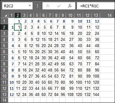
FIGURE 5-8 The macro creates a multiplication table. The formula in B2 uses two mixed references: =$A2*B$1.
![]() Caution
Caution
After running the macro and producing the multiplication table shown in Figure 5-8, note that Excel still has the copied range from line 2 of the macro as the active Clipboard item. If the user of this macro selects a cell and presses Enter, the contents of those cells copy to the new location. However, this is generally not desirable. To get Excel out of Cut/Copy mode, add this line of code before your program ends:
Application.CutCopyMode = False
An interesting twist
Try this experiment: Move the cell pointer to F6. Turn on macro recording using the Record Macro button on the Developer tab. Click the Use Relative Reference button on the Developer tab. Enter the formula =A1 and press Ctrl+Enter to stay in F6. Click the Stop Recording button on the floating toolbar. You get this single-line macro, which enters a formula that points to a cell five rows up and five columns to the left:
Sub Macro1()
   ActiveCell.FormulaR1C1 = "=R[-5]C[-5]"
End Sub
Now, move the cell pointer to cell A1 and run the macro that you just recorded. You might think that pointing to a cell five rows above A1 would lead to the ubiquitous Run Time Error 1004. But it doesn’t! When you run the macro, the formula in cell A1 is pointing to =XFA1048572, as shown in Figure 5-9, meaning that R1C1-style formulas actually wrap from the left side of the workbook to the right side. I cannot think of any instance in which this would actually be useful, but for those of you who rely on Excel to error out when you ask for something that does not make sense, be aware that your macro will happily provide a result that’s probably not the one that you expected!
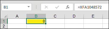
FIGURE 5-9 The formula to point to five rows above B1 wraps around to the bottom of the worksheet.
Remembering column numbers associated with column letters
I like R1C1-style formulas enough to use them regularly in VBA. I don’t like them enough to change my Excel interface over to R1C1-style numbers. So, I routinely have to know that the cell known as U21, for example, is really R21C21.
Knowing that U is the twenty-first letter of the alphabet is not something that comes naturally. We have 26 letters, so A is 1 and Z is 26. M is the halfway point of the alphabet and is column 13. The rest of the letters are not particularly intuitive. A quick way to get the column number for any column is to enter =COLUMN() in any empty cell in that column. The result tells you that, for example, DGX is column 2910 (see Figure 5-10).
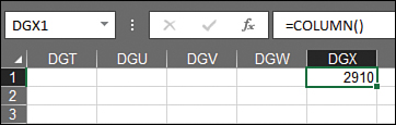
FIGURE 5-10 Use the temporary formula =COLUMN() to learn the column number of any cell.
You could also select any cell in DGX, switch to VBA, press Ctrl+G for the Immediate window, type ? ActiveCell.Column, and press Enter.
Next steps
This chapter covered a great technique of using R1C1 formulas to make your code easier to understand. In Chapter 6, you will see how to use Names in order to keep track of cells that might potentially be moved around by the person using the workbook.