
Chapter 22. Introduction to Storage and Storage Networking
This chapter covers the following exam topics:
4.0. Basic data center storage
4.1. Differentiate between file- and block-based storage protocols
4.2. Describe the roles of FC and FCoE port types
4.3. Describe the purpose of a VSAN
4.4. Describe the addressing model of block-based storage protocols
4.4.a. FC
4.4.b. iSCSI
Every day, thousands of devices are newly connected to the Internet. Devices previously only plugged into a power outlet are connected to the Internet and are sending and receiving tons of data. Powerful technology trends include the dramatic increase in processing power, storage, and bandwidth at ever-lower costs; the rapid growth of cloud, social media, and mobile computing; the ability to analyze Big Data and turn it into actionable information; and an improved ability to combine technologies (both hardware and software) in more powerful ways.
Companies are searching for more ways to efficiently manage expanding volumes of data, and to make that data accessible throughout the enterprise data centers. This demand is pushing the move of storage into the network. Storage area networks (SANs) are the leading storage infrastructure of today. SANs offer simplified storage management, scalability, flexibility, and availability, as well as improved data access, movement, and backup.
This chapter discusses the function and operation of the data center storage-networking technologies. It compares Small Computer System Interface (SCSI), Fibre Channel, and network-attached storage (NAS) connectivity for remote server storage. It covers Fibre Channel protocol and operations. This chapter goes directly into the edge/core layers of the SAN design and discusses topics relevant to the Introducing Cisco Data Center DCICN 200-150 certification.
“Do I Know This Already?” Quiz
The “Do I Know This Already?” quiz allows you to assess whether you should read this entire chapter thoroughly or jump to the “Exam Preparation Tasks” section. If you are in doubt about your answers to these questions or your own assessment of your knowledge of the topics, read the entire chapter. Table 22-1 lists the major headings in this chapter and their corresponding “Do I Know This Already?” quiz questions. You can find the answers in Appendix A, “Answers to the ‘Do I Know This Already?’ Quizzes.”

The goal of self-assessment is to gauge your mastery of the topics in this chapter. If you do not know the answer to a question or are only partially sure of the answer, you should mark that question as wrong for purposes of the self-assessment. Giving yourself credit for an answer you correctly guess skews your self-assessment results and might provide you with a false sense of security.
1. Which of the following options describe advantages of block-level storage systems? (Choose all the correct answers.)
a. Block-level storage systems are very popular with storage area networks.
b. They can support external boot of the systems connected to them.
c. Block-level storage systems are generally inexpensive when compared to file-level storage systems.
d. Each block or storage volume can be treated as an independent disk drive and is controlled by an external server OS.
e. Block-level storage systems are well suited for bulk file storage.
2. Which of the following options describe advantages of storage-area network (SAN)? (Choose all the correct answers.)
a. Consolidation
b. Storage virtualization
c. Business continuity
d. Secure access to all hosts
e. None
3. Which of the following protocols are file based? (Choose all the correct answers.)
a. CIFS
b. Fibre Channel
c. SCSI
d. NFS
4. Which options describe the characteristics of Tier 1 storage? (Choose all the correct answers.)
a. Integrated large scale disk array.
b. Centralized controller and cache system.
c. It is used for mission-critical applications.
d. Backup storage product.
5. Which of the following options should be taken into consideration during SAN design? (Choose all the correct answers.)
a. Port density and topology requirements
b. Device performance and oversubscription ratios
c. Traffic management
d. Low latency
6. Which of the following options are correct for Fibre Channel addressing? (Choose all the correct answers.)
a. A dual-ported HBA has three WWNs: one nWWN, and one pWWN for each port.
b. Every HBA, array controller, switch, gateway, and Fibre Channel disk drive has a single unique nWWN.
c. The domain ID is an 8-bit field, and only 239 domains are available to the fabric.
d. The arbitrated loop physical address (AL-PA) is a 16-bit address.
7. Which process allows an N Port to exchange information about ULP support with its target N Port to ensure that the initiator and target process can communicate?
a. FLOGI
b. PLOGI
c. PRLI
d. PRLO
8. Which type of port is used to create an ISL on a Fibre Channel SAN?
a. E
b. F
c. TN
d. NP
9. Which of the following options are correct for VSANs? (Choose all the correct answers)
a. An HBA or a storage device can belong to only a single VSAN—the VSAN associated with the Fx port.
b. An HBA or storage device can belong to multiple VSANs.
c. Membership is typically defined using the VSAN ID to Fx ports.
d. On a Cisco MDS switch, one can define 4096 VSANs.
10. Which of the following options are correct for iSCSI?
a. Uses TCP port 3225
b. Uses TCP port 3260
c. Uses UDP port 3225
d. Uses UDP port 3260
e. Uses both UDP and TCP
Foundation Topics
What Is a Storage Device?
Data is stored on hard disk drives that can be both read and written on. A hard disk drive (HDD) is a data storage device used for storing and retrieving digital information using rapidly rotating disks (platters) coated with magnetic material. An HDD retains its data even when powered off. Data is read in a random-access manner, meaning individual blocks of data can be stored or retrieved in any order rather than sequentially. Depending on the methods that are used to run those tasks, and the HDD technology on which they were built, the read and write function can be faster or slower.
IBM introduced the first HDD in 1956; HDDs became the dominant secondary storage device for general-purpose computers by the early 1960s. Continuously improved, HDDs have maintained this position into the modern era of servers and personal computers. More than 200 companies have produced HDD units. Most current units are manufactured by Seagate, Toshiba, and Western Digital.
The primary characteristics of an HDD are its capacity and performance. Capacity is specified in unit prefixes corresponding to powers of 1000: a 1-terabyte (TB) drive has a capacity of 1000 gigabytes (GB; where 1 gigabyte = 1 billion bytes). HDDs are accessed over one of a number of bus types, including (as of 2011) parallel ATA (PATA, also called IDE or EIDE; described before the introduction of SATA as ATA), Serial ATA (SATA), SCSI, Serial Attached SCSI (SAS), and Fibre Channel.
As of 2014, the primary competing technology for secondary storage is flash memory in the form of solid-state drives (SSDs). HDDs are expected to remain the dominant medium for secondary storage due to predicted continuing advantages in recording capacity, price per unit of storage, write latency, and product lifetime. SSDs are replacing HDDs where speed, power consumption, and durability are more important considerations.
The basic interface for all modern drives is straightforward. The drive consists of a large number of sectors (512-byte blocks), each of which can be read or written. The sectors are numbered from 0 to n – 1 on a disk with n sectors. Thus, we can view the disk as an array of sectors; 0 to n – 1 is therefore the address space of the drive. Multisector operations are possible; indeed, many file systems will read or write 4 KB at a time (or more). A platter is a circular hard surface on which data is stored persistently by inducing magnetic changes to it. A disk may have one or more platters; each platter has two sides, each of which is called a surface. These platters are usually made of some hard material (such as aluminum) and then coated with a thin magnetic layer that enables the drive to persistently store bits even when the drive is powered off.
The platters are all bound together around the spindle, which is connected to a motor that spins the platters around (while the drive is powered on) at a constant (fixed) rate. The rate of rotation is often measured in rotations per minute (RPM), and typical modern values are in the 7200 RPM to 15,000 RPM range. Note that we will often be interested in the time of a single rotation; for example, a drive that rotates at 10,000 RPM means that a single rotation takes about 6 milliseconds (6 ms).
Data is encoded on each surface in concentric circles of sectors; we call one such concentric circle a track. There are usually 1024 tracks on a single disk, and all corresponding tracks from all disks define a cylinder (see Figure 22-1).

A specific sector must be referenced through a three-part address composed of cylinder/head/sector information. And cache is just some small amount of memory (usually around 8 or 16 MB) that the drive can use to hold data read from or written to the disk. For example, when reading a sector from the disk, the drive might decide to read in all of the sectors on that track and cache them in its memory; doing so allows the drive to quickly respond to any subsequent requests to the same track. Although the internal system of cylinders, tracks, and sectors is interesting, it is also not used much anymore by the systems and subsystems that use disk drives. Cylinder, track, and sector addresses have been replaced by a method called logical block addressing (LBA), which makes disks much easier to work with by presenting a single flat address space. To a large degree, logical block addressing facilitates the flexibility of storage networks by allowing many types of disk drives to be integrated more easily into a large heterogeneous storage environment.
The most widespread standard for configuring multiple hard drives is RAID (Redundant Array of Inexpensive/Independent Disks), which comes in a number of standard configurations and nonstandard configurations. Data is distributed across the drives in one of several ways, referred to as RAID levels, depending on the specific level of redundancy and performance required. The different schemes or architectures are named by the word RAID followed by a number (RAID 0, RAID 1, and so on). Each scheme provides a different balance between the key goals: reliability, availability, performance, and capacity. RAID levels greater than RAID 0 provide protection against unrecoverable (sector) read errors as well as whole disk failure. JBOD (derived from “just a bunch of disks”) is an architecture involving multiple hard drives, making them accessible either as independent hard drives or as a combined (spanned) single logical volume with no actual RAID functionality. Hard drives may be handled independently as separate logical volumes, or they may be combined into a single logical volume using a volume manager.
Typically, a disk array provides increased availability, resiliency, and maintainability by using existing components (controllers, power supplies, fans, disk enclosures, access ports, cache, and so on), often up to the point where all single points of failure (SPOFs) are eliminated from the design. Additionally, disk array components are often hot swappable. Disk arrays are divided into the following categories:
![]() Network-attached storage (NAS) arrays are based on file-level storage. In this type of storage, the storage disk is configured with a particular protocol (such as NFS, CIFS, and so on) and files are stored and accessed from it as such, in bulk.
Network-attached storage (NAS) arrays are based on file-level storage. In this type of storage, the storage disk is configured with a particular protocol (such as NFS, CIFS, and so on) and files are stored and accessed from it as such, in bulk.
Advantages of file-level storage systems are the following:
![]() File-level storage systems are simple to implement and simple to use.
File-level storage systems are simple to implement and simple to use.
![]() They store files and folders and are visible as such to both the systems storing the files and the systems accessing them.
They store files and folders and are visible as such to both the systems storing the files and the systems accessing them.
![]() File-level storage systems are generally inexpensive when compared to block-level storage systems.
File-level storage systems are generally inexpensive when compared to block-level storage systems.
![]() File-level storage systems are more popular with NAS-based storage systems.
File-level storage systems are more popular with NAS-based storage systems.
![]() They can be configured with common file-level protocols such as NTFS (Windows), NFS (Linux), and so on.
They can be configured with common file-level protocols such as NTFS (Windows), NFS (Linux), and so on.
![]() File-level storage systems are well suited for bulk file storage.
File-level storage systems are well suited for bulk file storage.
The file-level storage device itself can generally handle operations such as access control, integration with corporate directories, and the like.
![]() Storage-area network (SAN) arrays are based on block-level storage. The raw blocks (storage volumes) are created, and each block can be controlled like an individual hard drive. Generally, these blocks are controlled by the server-based operating systems. Each block or storage volume can be individually formatted with the required file system.
Storage-area network (SAN) arrays are based on block-level storage. The raw blocks (storage volumes) are created, and each block can be controlled like an individual hard drive. Generally, these blocks are controlled by the server-based operating systems. Each block or storage volume can be individually formatted with the required file system.
Advantages of block level storage systems are the following:
![]() Block-level storage systems offer better performance and speed than file-level storage systems.
Block-level storage systems offer better performance and speed than file-level storage systems.
![]() Each block or storage volume can be treated as an independent disk drive and is controlled by the external server OS.
Each block or storage volume can be treated as an independent disk drive and is controlled by the external server OS.
![]() Each block or storage volume can be formatted with the file system required by the application (NFS/NTFS/SMB).
Each block or storage volume can be formatted with the file system required by the application (NFS/NTFS/SMB).
![]() Block-level storage systems are very popular with SANs.
Block-level storage systems are very popular with SANs.
![]() Block-level storage systems are more reliable, and their transport systems are very efficient.
Block-level storage systems are more reliable, and their transport systems are very efficient.
![]() Block-level storage can be used to store files and also provide the storage required for special applications such as databases, Virtual Machine File Systems (VMFSs), and the like.
Block-level storage can be used to store files and also provide the storage required for special applications such as databases, Virtual Machine File Systems (VMFSs), and the like.
![]() They can support external boot of the systems connected to them.
They can support external boot of the systems connected to them.
Primary vendors of storage systems include EMC Corporation, Hitachi Data Systems, NetApp, IBM, Hewlett-Packard, Oracle Corporation, Dell, Infortrend, and other companies that often act as OEMs for the previously mentioned vendors and do not themselves market the storage components they manufacture.
Servers are connected to the connection port of the disk subsystem using standard I/O techniques such as Small Computer System Interface (SCSI), Fibre Channel, and Internet SCSI (iSCSI) and can thus use the storage capacity that the disk subsystem provides (see Figure 22-2). The internal structure of the disk subsystem is completely hidden from the server, which sees only the hard disks that the disk subsystem provides to the server.
Direct-attached storage (DAS) is often implemented within a parallel SCSI implementation. DAS is commonly described as captive storage. Devices in a captive storage topology do not have direct access to the storage network and do not support efficient sharing of storage. To access data with DAS, a user must go through some sort of front-end network. DAS devices provide little or no mobility to other servers and little scalability. DAS devices limit file sharing and can be complex to implement and manage. For example, to support data backups, DAS devices require resources on the host and spare disk systems that cannot be used on other systems.

The controller of the disk subsystem must ultimately store all data on physical hard disks. Standard I/O techniques such as SCSI, Fibre Channel, and increasingly Serial ATA (SATA), Serial Attached SCSI (SAS), and Serial Storage Architecture (SSA) are being used for internal I/O channels between connection ports and the controller as well as between the controller and internal hard disks. Sometimes, however, proprietary—that is, manufacturer-specific—I/O techniques are used. The I/O channels can be designed with built-in redundancy to increase the fault-tolerance of a disk subsystem. There are four main I/O channel designs:
![]() Active: In active cabling, the individual physical hard disks are connected via only one I/O channel; if this access path fails, it is no longer possible to access the data.
Active: In active cabling, the individual physical hard disks are connected via only one I/O channel; if this access path fails, it is no longer possible to access the data.
![]() Active/passive: In active/passive cabling, the individual hard disks are connected via two I/O channels; in normal operation the controller communicates with the hard disks via the first I/O channel, and the second I/O channel is not used. In the event of the failure of the first I/O channel, the disk subsystem switches from the first to the second I/O channel.
Active/passive: In active/passive cabling, the individual hard disks are connected via two I/O channels; in normal operation the controller communicates with the hard disks via the first I/O channel, and the second I/O channel is not used. In the event of the failure of the first I/O channel, the disk subsystem switches from the first to the second I/O channel.
![]() Active/active (no load sharing): In this cabling method, the controller uses both I/O channels in normal operation. The hard disks are divided into two groups: in normal operation the first group is addressed via the first I/O channel and the second via the second I/O channel. If one I/O channel fails, both groups are addressed via the other I/O channel.
Active/active (no load sharing): In this cabling method, the controller uses both I/O channels in normal operation. The hard disks are divided into two groups: in normal operation the first group is addressed via the first I/O channel and the second via the second I/O channel. If one I/O channel fails, both groups are addressed via the other I/O channel.
![]() Active/active (load sharing): In this approach, all hard disks are addressed via both I/O channels; in normal operation, the controller divides the load dynamically between the two I/O channels so that the available hardware can be optimally utilized. If one I/O channel fails, the communication goes through the other channel only.
Active/active (load sharing): In this approach, all hard disks are addressed via both I/O channels; in normal operation, the controller divides the load dynamically between the two I/O channels so that the available hardware can be optimally utilized. If one I/O channel fails, the communication goes through the other channel only.
A tape drive is a data storage device that reads and writes data on a magnetic tape. Magnetic tape data storage is typically used for offline, archival data storage. A tape drive provides sequential access storage, unlike a disk drive, which provides random access storage. A disk drive can move to any position on the disk in a few milliseconds, but a tape drive must physically wind tape between reels to read any one particular piece of data. As a result, tape drives have very slow average seek times for sequential access after the tape is positioned. However, tape drives can stream data very quickly. For example, as of 2010, Linear Tape-Open (LTO) supported continuous data transfer rates of up to 140 MBps, comparable to hard disk drives. A tape library, sometimes called a tape silo, tape robot, or tape jukebox, is a storage device that contains one or more tape drives, a number of slots to hold tape cartridges, a bar-code reader to identify tape cartridges, and an automated method for loading tapes (a robot). These devices can store immense amounts of data, currently ranging from 20 TB up to 2.1 EB (exabytes) of data or multiple thousand times the capacity of a typical hard drive and well in excess of capacities achievable with network-attached storage.
We talked about block-level and file-level storage. Now it is time to extend your knowledge to object storage. Object storage is not directly accessed by the operating system. It is not seen as a local or a remote file system. Instead, interaction occurs at the application level via an API. Block-level storage and file-level storage are designed to be consumed by the operating system; object storage is designed to be consumed by the application. Object storage devices offer the ability to aggregate storage into disparate grid storage structures that undertake work traditionally performed by single subsystems while providing load distribution capabilities and resilience far in excess of that available in a traditional SAN environment. Object storage devices operate as modular units that can become components of a larger storage pool and can be aggregated across locations. The advantages of this are considerable because distributed storage nodes can provide options to increase data resilience and enable disaster recovery strategies.
To better understand the object structure, think of the objects as the cells in a beehive. Each cell is a self-contained repository for an object ID number, metadata, data attributes, and the stored data itself. Each cell is also a separate object within the usable disk space pool.
Physically, object-based storage arrays are composed of stackable, self-contained disk units like any other SAN. Unlike traditional storage arrays, object-based systems are accessed via HTTP. That access method plus their ability to scale to petabytes of data make object-based systems a good choice for public cloud storage. An entire object storage cluster of disparate nodes can be easily combined to become an online, scalable file repository. Object storage works very well for unstructured data sets where data is generally read but not written to. Static web content, data backups and archival images, and multimedia (videos, pictures, or music) files are best stored as objects. Databases in an object storage environment ideally have data sets that are unstructured, where the use cases suggest the data will not require a large number of writes or incremental updates. Object storage is used for diverse purposes such as storing photos on Facebook, songs on Spotify, or files in online collaboration services such as Dropbox.
In the rapidly evolving landscape of enterprise data storage, one thing is clear: We need to store more data, more simply, more efficiently, and for a lower overall cost. Object storage addresses these issues without expensive custom hardware that will need to be replaced every few years. As we enter an age of zettabytes of data, more and more enterprises are turning to object storage as their go-to storage solution.
What Is Storage Area Network?
The Storage Networking Industry Association (SNIA) defines the storage-area network (SAN) as a network whose primary purpose is the transfer of data between computer systems and storage elements and among storage elements. A SAN consists of a communication infrastructure, which provides physical connections and a management layer. This layer organizes the connections, storage elements, and computer systems so that data transfer is secure and robust. The term SAN is usually (but not necessarily) identified with block I/O services rather than file-access services. A SAN is a specialized, high-speed network that attaches servers and storage devices. A SAN allows an any-to-any connection across the network by using interconnect elements such as switches and directors. It eliminates the traditional dedicated connection between a server and storage, and the concept that the server effectively owns and manages the storage devices. It also eliminates any restriction to the amount of data that a server can access, currently limited by the number of storage devices attached to the individual server. Instead, a SAN introduces the flexibility of networking to enable one server or many heterogeneous servers to share a common storage utility. A network might include many storage devices, including disk, tape, and optical storage. Additionally, the storage utility might be located far from the servers that it uses. Figure 22-3 portrays a sample SAN topology.

The key benefits that a storage area network (SAN) might bring to a highly data-dependent business infrastructure can be summarized into three concepts: simplification of the infrastructure, information life-cycle management (ILS), and business continuity.
The simplification of the infrastructure consists of six main areas:
![]() Consolidation: Involves concentrating the systems and resources into locations with fewer, but more powerful, servers and storage pools that can help increase IT efficiency and simplify the infrastructure. In addition, centralized storage management tools can help improve scalability, availability, and disaster tolerance.
Consolidation: Involves concentrating the systems and resources into locations with fewer, but more powerful, servers and storage pools that can help increase IT efficiency and simplify the infrastructure. In addition, centralized storage management tools can help improve scalability, availability, and disaster tolerance.
![]() Storage virtualization: Helps in making complexity nearly transparent and can offer a composite view of storage assets. We will be talking about storage virtualization in detail in Chapter 23, “Advanced Data Center Storage.”
Storage virtualization: Helps in making complexity nearly transparent and can offer a composite view of storage assets. We will be talking about storage virtualization in detail in Chapter 23, “Advanced Data Center Storage.”
![]() Automation: Involves choosing storage components with autonomic capabilities, which can improve availability and responsiveness and can help protect data as storage needs grow. As soon as day-to-day tasks are automated, storage administrators might be able to spend more time on critical, higher-level tasks that are unique to the company’s business mission.
Automation: Involves choosing storage components with autonomic capabilities, which can improve availability and responsiveness and can help protect data as storage needs grow. As soon as day-to-day tasks are automated, storage administrators might be able to spend more time on critical, higher-level tasks that are unique to the company’s business mission.
![]() Integrated storage environments: Simplify system management tasks and improve security. When all servers have secure access to all data, your infrastructure might be better able to respond to the information needs of your users.
Integrated storage environments: Simplify system management tasks and improve security. When all servers have secure access to all data, your infrastructure might be better able to respond to the information needs of your users.
![]() Information life-cycle management (ILM): A process for managing information through its life cycle, from conception until intentional disposal. The ILM process manages this information in a manner that optimizes storage and maintains a high level of access at the lowest cost. A SAN implementation makes it easier to manage the information life cycle because it integrates applications and data into a single-view system in which the information resides.
Information life-cycle management (ILM): A process for managing information through its life cycle, from conception until intentional disposal. The ILM process manages this information in a manner that optimizes storage and maintains a high level of access at the lowest cost. A SAN implementation makes it easier to manage the information life cycle because it integrates applications and data into a single-view system in which the information resides.
![]() Business continuity (BC): Involves building and improving resilience in your business; it’s about identifying your key products and services and the most urgent activities that underpin them; then, after that analysis is complete, it is about devising plans and strategies that will enable you to continue your business operations and enable you to recover quickly and effectively from any type of disruption, whatever its size or cause. It gives you a solid framework to lean on in times of crisis and provides stability and security. In fact, embedding BC into your business is proven to bring business benefits. SANs play a key role in the business continuity. By deploying a consistent and safe infrastructure, SANs make it possible to meet any availability requirements.
Business continuity (BC): Involves building and improving resilience in your business; it’s about identifying your key products and services and the most urgent activities that underpin them; then, after that analysis is complete, it is about devising plans and strategies that will enable you to continue your business operations and enable you to recover quickly and effectively from any type of disruption, whatever its size or cause. It gives you a solid framework to lean on in times of crisis and provides stability and security. In fact, embedding BC into your business is proven to bring business benefits. SANs play a key role in the business continuity. By deploying a consistent and safe infrastructure, SANs make it possible to meet any availability requirements.
Fibre Channel is a serial I/O interconnect that is capable of supporting multiple protocols, including access to open system storage (FCP), access to mainframe storage (FICON), and networking (TCP/IP). Fibre Channel supports point-to-point, arbitrated loop, and switched topologies with various copper and optical links that are running at speeds from 1 Gbps to 16 Gbps. The committee that is standardizing Fibre Channel is the INCITS Fibre Channel (T11) Technical Committee.
A storage system consists of storage elements, storage devices, computer systems, and appliances, plus all control software that communicates over a network. Storage subsystems, storage devices, and server systems can be attached to a Fibre Channel SAN. Depending on the implementation, several components can be used to build a SAN. It is, as the name suggests, a network, so any combination of devices that is able to interoperate is likely to be used. Given this definition, a Fibre Channel network might be composed of many types of interconnect entities, including directors, switches, hubs, routers, gateways, and bridges. It is the deployment of these different types of interconnect entities that allows Fibre Channel networks of varying scales to be built. In smaller SAN environments you can deploy hubs for Fibre Channel arbitrated loop topologies, or switches and directors for Fibre Channel switched fabric topologies. As SANs increase in size and complexity, Fibre Channel directors can be introduced to facilitate a more flexible and fault-tolerant configuration. Each of the components that compose a Fibre Channel SAN provides an individual management capability and participates in an often-complex end-to-end management environment.
How to Access a Storage Device
Each new storage technology introduced a new physical interface, electrical interface, and storage protocol. The intelligent interface model abstracts device-specific details from the storage protocol and decouples the storage protocol from the physical and electrical interfaces. This allows multiple storage technologies to use a common storage protocol. In this chapter, we will be categorizing them in three major groups:
![]() Blocks: Sometimes called a physical record, a block is a sequence of bytes or bits, usually containing some whole number of records having a maximum length (a block size). This type of structured data is called “blocked.” Most file systems are based on a block device, which is a level of abstraction for the hardware responsible for storing and retrieving specified blocks of data, although the block size in file systems may be a multiple of the physical block size.
Blocks: Sometimes called a physical record, a block is a sequence of bytes or bits, usually containing some whole number of records having a maximum length (a block size). This type of structured data is called “blocked.” Most file systems are based on a block device, which is a level of abstraction for the hardware responsible for storing and retrieving specified blocks of data, although the block size in file systems may be a multiple of the physical block size.
![]() Files: Files are granular containers of data created by the system or an application. By separating the data into individual pieces and giving each piece a name, the information is easily separated and identified. The structure and logic rule used to manage the groups of information and their names is called a “file system.” Some file systems are used on local data storage devices; others provide file access via a network protocol.
Files: Files are granular containers of data created by the system or an application. By separating the data into individual pieces and giving each piece a name, the information is easily separated and identified. The structure and logic rule used to manage the groups of information and their names is called a “file system.” Some file systems are used on local data storage devices; others provide file access via a network protocol.
![]() Records: Records are similar to the file system. There are several record formats; the details vary depending on the particular system. In general, the formats can be fixed length or variable length, with different physical organizations or padding mechanisms; metadata may be associated with the file records to define the record length, or the data may be part of the record. Different methods to access records may be provided—for example, sequential, by key, or by record number.
Records: Records are similar to the file system. There are several record formats; the details vary depending on the particular system. In general, the formats can be fixed length or variable length, with different physical organizations or padding mechanisms; metadata may be associated with the file records to define the record length, or the data may be part of the record. Different methods to access records may be provided—for example, sequential, by key, or by record number.
Block-Level Protocols
Block-oriented protocols (also known as block-level protocols) read and write individual fixed-length blocks of data. Small Computer Systems Interface (SCSI) is a block-level I/O protocol for writing and reading data blocks to and from a storage device. Data transfer is also governed by standards. SCSI is an American National Standards Institute (ANSI) standard that is one of the leading I/O buses in the computer industry. The SCSI bus is a parallel bus, which comes in a number of variants, as shown in Table 22-2. The first version of the SCSI standard was released in 1986. Since then, SCSI has been continuously developed.
The International Committee for Information Technology Standards (INCITS) is the forum of choice for information technology developers, producers, and users for the creation and maintenance of formal daily IT standards. INCITS is accredited by and operates under rules approved by the American National Standards Institute (ANSI). These rules are designed to ensure that voluntary standards are developed by the consensus of directly and materially affected interests. The Information Technology Industry Council (ITI) sponsors INCITS (see Figure 22-4). The standard process is that a technical committee (T10, T11, T13) prepares drafts. Drafts are sent to INCITS for approval. After the drafts are approved by INCITS, they become standards and are published by ANSI. ANSI promotes American National Standards to ISO as a joint technical committee member (JTC-1).

As a medium, SCSI defines a parallel bus for the transmission of data with additional lines for the control of communication. The bus can be realized in the form of printed conductors on the circuit board or as a cable. Over time, numerous cable and plug types have been defined that are not directly compatible with one another (see Table 22-2). A so-called “daisy chain” can connect up to 16 devices together.

All SCSI devices are intelligent, but SCSI operates as a master/slave model. One SCSI device (the initiator) initiates communication with another SCSI device (the target) by issuing a command, to which a response is expected. Thus, the SCSI protocol is half-duplex by design and is considered a command/response protocol.
The initiating device is usually a SCSI controller, so SCSI controllers typically are called initiators. SCSI storage devices typically are called targets (see Figure 22-5). A SCSI controller in a modern storage array acts as a target externally and acts as an initiator internally. Also note that array-based replication software requires a storage controller in the initiating storage array to act as initiator both externally and internally. SCSI targets have logical units that provide the processing context for SCSI commands. Essentially, a logical unit is a virtual machine (or virtual controller) that handles SCSI communications on behalf of real or virtual storage devices in a target. Commands received by targets are directed to the appropriate logical unit by a task router in the target controller.

The logical unit number (LUN) identifies a specific logical unit (virtual controller) in a target. Although we tend to use the term LUN to refer to a real or virtual storage device, a LUN is an access point for exchanging commands and status information between initiators and targets. A logical unit can be thought of as a “black box” processor, and the LUN is a way to identify SCSI black boxes. Logical units are architecturally independent of target ports and can be accessed through any of the target’s ports, via a LUN. A target must have at least one LUN, LUN 0, and might optionally support additional LUNs. For instance, a disk drive might use a single LUN, whereas a subsystem might allow hundreds of LUNs to be defined.
The process of provisioning storage in a SAN storage subsystem involves defining a LUN on a particular target port and then assigning that particular target/LUN pair to a specific logical unit. An individual logical unit can be represented by multiple LUNs on different ports. For instance, a logical unit could be accessed through LUN 1 on Port 0 of a target and also accessed as LUN 8 on port 1 of the same target.
The bus, target, and LUN triad is defined from parallel SCSI technology. The bus represents one of several potential SCSI interfaces that are installed in the host, each supporting a separate string of disks. The target represents a single disk controller on the string. Depending on the version of the SCSI standard, a maximum of 8 or 16 IDs are permitted per SCSI bus. A server can be equipped with several SCSI controllers. Therefore, the operating system must note three things for the differentiation of devices: controller ID, SCSI ID, and LUN. The SCSI protocol permitted only eight IDs, with ID 7 having the highest priority. More recent versions of the SCSI protocol permit 16 different IDs. For reasons of compatibility, IDs 7 to 0 should retain the highest priority so that IDs 15 to 8 have a lower priority (see Figure 22-6).
Devices (servers and storage devices) must reserve the SCSI bus (arbitrate) before they may send data through it. During the arbitration of the bus, the device that has the highest priority SCSI ID always wins. In the event that the bus is heavily loaded, this can lead to devices with lower priorities never being allowed to send data. The SCSI arbitration procedure is therefore “unfair.”

The SCSI protocol layer sits between the operating system and the peripheral resources, so it has different functional components (see Figure 22-7). Applications typically access data as files or records. Although this information might be stored on disk or tape media in the form of data blocks, retrieval of the file requires a hierarchy of functions. These functions assemble raw data blocks into a coherent file that an application can manipulate.
It is important to understand that whereas SCSI-1 and SCSI-2 represent actual standards that completely define SCSI (connectors, cables, signals, and command protocol), SCSI-3 is an all-encompassing term that refers to a collection of standards that were written as a result of breaking SCSI-2 into smaller, hierarchical modules that fit within a general framework called SCSI Architecture Model (SAM).
The SCSI version 3 (SCSI-3) application client resides in the host and represents the upper layer application, file system, and operating system I/O requests. The SCSI-3 device server sits in the target device, responding to requests. It is often also assumed that SCSI provides in-order delivery to maintain data integrity. In-order delivery was traditionally provided by the SCSI bus and, therefore, was not needed by the SCSI protocol layer. In SCSI-3, the SCSI protocol assumes that proper ordering is provided by the underlying connection technology. In other words, the SCSI protocol does not provide its own reordering mechanism, and the network is responsible for the reordering of transmission frames that are received out of order. This is the main reason why TCP was considered essential for the iSCSI protocol that transports SCSI commands and data transfers over IP networking equipment: TCP provided ordering while other upper-layer protocols, such as UDP, did not. In SCSI-3, even faster bus types are introduced, along with serial SCSI buses that reduce the cabling overhead and allow a higher maximum bus length. It is at this point where the Fibre Channel model is introduced. As always, the demands and needs of the market push for new technologies. In particular, there is always a push for faster communications without limitations on distance or on the number of connected devices.

The SCSI protocol is suitable for block-based, structured applications such as database applications that require many I/O operations per second (IOPS) to achieve high performance. IOPS (input/output operations per second, pronounced eye-ops) is a common performance measurement used to benchmark computer storage devices like hard disk drives (HDDs), solid-state drives (SSDs), and storage-area networks (SANs). The specific number of IOPS possible in any system configuration will vary greatly, depending on the variables the tester enters into the program, including the balance of read and write operations, the mix of sequential and random-access patterns, the number of worker threads and queue depth, as well as the data block sizes.
For HDDs and similar electromechanical storage devices, the random IOPS numbers are primarily dependent on the storage device’s random seek time, whereas for SSDs and similar solid-state storage devices, the random IOPS numbers are primarily dependent on the storage device’s internal controller and memory interface speeds. On both types of storage devices, the sequential IOPS numbers (especially when using a large block size) typically indicate the maximum sustained bandwidth that the storage device can handle. Often, sequential IOPS are reported as a simple MBps number, as follows:
IOPS × TransferSizeInBytes = BytesPerSec (and typically this is converted to megabytes per second)
SCSI messages and data can be transported in several ways:
![]() Parallel SCSI cable: This transport is mainly used in traditional deployments. Latency is low, but distance is limited to 25 m and is half-duplex, so data can flow in only one direction at a time.
Parallel SCSI cable: This transport is mainly used in traditional deployments. Latency is low, but distance is limited to 25 m and is half-duplex, so data can flow in only one direction at a time.
![]() iSCSI is SCSI over TCP/IP: Internet Small Computer System Interface (iSCSI) is a transport protocol that carries SCSI commands from an initiator to a target. It is a data storage networking protocol that transports standard SCSI requests over the standard Transmission Control Protocol/Internet Protocol (TCP/IP) networking technology. iSCSI enables the implementation of IP-based SANs, enabling clients to use the same networking technologies for both storage and data networks. Because it uses TCP/IP, iSCSI is also suited to run over almost any physical network. By eliminating the need for a second network technology just for storage, iSCSI has the potential to lower the costs of deploying networked storage.
iSCSI is SCSI over TCP/IP: Internet Small Computer System Interface (iSCSI) is a transport protocol that carries SCSI commands from an initiator to a target. It is a data storage networking protocol that transports standard SCSI requests over the standard Transmission Control Protocol/Internet Protocol (TCP/IP) networking technology. iSCSI enables the implementation of IP-based SANs, enabling clients to use the same networking technologies for both storage and data networks. Because it uses TCP/IP, iSCSI is also suited to run over almost any physical network. By eliminating the need for a second network technology just for storage, iSCSI has the potential to lower the costs of deploying networked storage.
![]() Fibre Channel cable: This transport is the basis for a traditional SAN deployment. Latency is low and bandwidth is high (16 GBps). SCSI is carried in the payload of a Fibre Channel frame between Fibre Channel ports. Fibre Channel has a lossless delivery mechanism by using buffer-to-buffer credits (BB_Credits), which we explain in detail later in this chapter.
Fibre Channel cable: This transport is the basis for a traditional SAN deployment. Latency is low and bandwidth is high (16 GBps). SCSI is carried in the payload of a Fibre Channel frame between Fibre Channel ports. Fibre Channel has a lossless delivery mechanism by using buffer-to-buffer credits (BB_Credits), which we explain in detail later in this chapter.
![]() Fibre Channel connection (FICON): This architecture is an enhancement of, rather than a replacement for, the traditional IBM Enterprise Systems Connection (ESCON) architecture. A SAN is Fibre Channel based (FC based). Therefore, FICON is a prerequisite for IBM z/OS systems to fully participate in a heterogeneous SAN, where the SAN switch devices allow the mixture of open systems and mainframe traffic. FICON is a protocol that uses Fibre Channel as its physical medium. FICON channels can achieve data rates up to 850 MBps and extend the channel distance (up to 100 km). At the time of writing this book, FICON can also increase the number of control unit images per link and the number of device addresses per control unit link. The protocol can also retain the topology and switch management characteristics of ESCON.
Fibre Channel connection (FICON): This architecture is an enhancement of, rather than a replacement for, the traditional IBM Enterprise Systems Connection (ESCON) architecture. A SAN is Fibre Channel based (FC based). Therefore, FICON is a prerequisite for IBM z/OS systems to fully participate in a heterogeneous SAN, where the SAN switch devices allow the mixture of open systems and mainframe traffic. FICON is a protocol that uses Fibre Channel as its physical medium. FICON channels can achieve data rates up to 850 MBps and extend the channel distance (up to 100 km). At the time of writing this book, FICON can also increase the number of control unit images per link and the number of device addresses per control unit link. The protocol can also retain the topology and switch management characteristics of ESCON.
![]() Fibre Channel over IP (FCIP): Also known as Fibre Channel tunneling or storage tunneling. It is a method to allow the transmission of Fibre Channel information to be tunneled through the IP network. Because most organizations already have an existing IP infrastructure, the attraction of being able to link geographically dispersed SANs, at a relatively low cost, is enormous.
Fibre Channel over IP (FCIP): Also known as Fibre Channel tunneling or storage tunneling. It is a method to allow the transmission of Fibre Channel information to be tunneled through the IP network. Because most organizations already have an existing IP infrastructure, the attraction of being able to link geographically dispersed SANs, at a relatively low cost, is enormous.
FCIP encapsulates Fibre Channel block data and then transports it over a TCP socket. TCP/IP services are used to establish connectivity between remote SANs. Any congestion control and management and data error and data loss recovery is handled by TCP/IP services and does not affect Fibre Channel fabric services.
The major consideration with FCIP is that it does not replace Fibre Channel with IP; it allows deployments of Fibre Channel fabrics by using IP tunneling. The assumption that this might lead to is that the industry decided that Fibre Channel–based SANs are more than appropriate. Another possible assumption is that the only need for the IP connection is to facilitate any distance requirement that is beyond the current scope of an FCP SAN.
![]() Fibre Channel over Ethernet (FCoE): This transport replaces the Fibre Channel cabling with 10 Gigabit Ethernet cables and provides lossless delivery over converged I/O. FCoE will be discussed in detail in Chapter 23.
Fibre Channel over Ethernet (FCoE): This transport replaces the Fibre Channel cabling with 10 Gigabit Ethernet cables and provides lossless delivery over converged I/O. FCoE will be discussed in detail in Chapter 23.
Figure 22-8 portrays a networking stack comparison for all block I/O protocols.

Fibre Channel provides high-speed transport for SCSI payload via a host bus adapter (HBA), as shown in Figure 22-9. HBAs are I/O adapters that are designed to maximize performance by performing protocol-processing functions in silicon. HBAs are roughly analogous to network interface cards (NICs), but HBAs are optimized for SANs and provide features that are specific to storage. Fibre Channel overcomes many shortcomings of Parallel I/O, including addressing for up to 16 million nodes, loop (shared) and fabric (switched) transport, host speeds of 100 to 1600 MBps (1–16 Gbps), support for multiple protocols, and combines the best attributes of a channel and a network together.

With NICs, software drivers perform protocol-processing functions such as flow control, sequencing, segmentation and reassembly, and error correction. The HBA offloads these protocol-processing functions onto the HBA hardware with some combination of an ASIC and firmware. Offloading these functions is necessary to provide the performance that storage networks require.
Fibre Channel Protocol (FCP) has an ANSI-based layered architecture that can be considered a general transport vehicle for upper layer protocols (ULPs) such as SCSI command sets, HIPPI data framing, IP, and others. Figure 22-10 shows an overview of the Fibre Channel model. The diagram shows the Fibre Channel, which is divided into four lower layers (FC-0, FC-1, FC-2, and FC-3) and one upper layer (FC-4). FC-4 is where the upper-level protocols are used, such as SCSI-3, Internet Protocol (IP), and Fibre Channel connection (FICON).

Here are the main functions of each Fibre Channel layer:
![]() FC-4 upper-layer protocol (ULP) mapping: Provides protocol mapping to identify the upper-level protocol (ULP) that is encapsulated into a protocol data unit (PDU) for delivery to the FC-2 layer.
FC-4 upper-layer protocol (ULP) mapping: Provides protocol mapping to identify the upper-level protocol (ULP) that is encapsulated into a protocol data unit (PDU) for delivery to the FC-2 layer.
![]() FC-3 generic services: Provides the Fibre Channel Generic Services (FC-GS) that are required for fabric management. Specifications exist here but are rarely implemented.
FC-3 generic services: Provides the Fibre Channel Generic Services (FC-GS) that are required for fabric management. Specifications exist here but are rarely implemented.
![]() FC-2 framing and flow control: Provides the framing and flow control that are required to transport the ULP over Fibre Channel. FC-2 functions include several classes of service, frame format definition, sequence disassembly and reassembly, exchange management, address assignment, alias address definition, protocols for hunt group, and multicast management and stacked connect requests.
FC-2 framing and flow control: Provides the framing and flow control that are required to transport the ULP over Fibre Channel. FC-2 functions include several classes of service, frame format definition, sequence disassembly and reassembly, exchange management, address assignment, alias address definition, protocols for hunt group, and multicast management and stacked connect requests.
![]() FC-1 encoding: Defines the transmission protocol that includes the serial encoding, decoding, and error control.
FC-1 encoding: Defines the transmission protocol that includes the serial encoding, decoding, and error control.
![]() FC-0 physical interface: Provides physical connectivity, including cabling, connectors, and so on.
FC-0 physical interface: Provides physical connectivity, including cabling, connectors, and so on.
Table 22-3 shows the evolution of Fibre Channel speeds. Fibre Channel is described in greater depth throughout this chapter. FCP is the FC-4 mapping of SCSI-3 onto FC. Fibre Channel throughput is commonly expressed in bytes per second rather than bits per second. In the initial FC specification, rates of 12.5 MBps, 25 MBps, 50 MBps, and 100 MBps were introduced on several different copper and fiber media. Additional rates were subsequently introduced, including 200 MBps and 400 MBps. 100 MBps FC is also known as 1Gbps FC, 200 MBps as 2Gbps FC, and 400 MBps as 4Gbps FC. The FC-PH specification defines baud rate as the encoded bit rate per second, which means the baud rate and raw bit rate are equal. The FC-PI specification redefines baud rate more accurately and states explicitly that FC encodes 1 bit per baud. FC-1 variants up to and including 8 Gbps use the same encoding scheme (8B/10B) as GE fiber-optic variants. 1Gbps FC operates at 1.0625 GBaud, provides a raw bit rate of 1.0625 Gbps, and provides a data bit rate of 850 Mbps. 2Gbps FC operates at 2.125 GBaud, provides a raw bit rate of 2.125 Gbps, and provides a data bit rate of 1.7 Gbps. 4Gbps FC operates at 4.25 GBaud, provides a raw bit rate of 4.25 Gbps, and provides a data bit rate of 3.4 Gbps. To derive ULP throughput, the FC-2 header and interframe spacing overhead must be subtracted. Note that FCP does not define its own header. Instead, fields within the FC-2 header are used by FCP. The basic FC-2 header adds 36 bytes of overhead. Inter-frame spacing adds another 24 bytes. Assuming the maximum payload (2112 bytes) and no optional FC-2 headers, the ULP throughput rate is 826.519 Mbps, 1.65304 Gbps, and 3.30608 Gbps for 1Gbps FC, 2Gbps FC, and 4Gbps FC, respectively. These ULP throughput rates are available directly to SCSI. The 1Gbps FC, 2Gbps FC, 4Gbps FC, and 8Gbps FC designs all use 8b/10b encoding, and the 10G and 16G FC standards use 64b/66b encoding. Unlike the 10Gbps FC standards, 16Gbps FC provides backward compatibility with 4Gbps FC and 8Gbps FC.

File-Level Protocols
File-oriented protocols (also known as file-level protocols) read and write variable-length files. Files are segmented into blocks before being stored on disk or tape. Common Internet File System (CIFS) and Network File System (NFS) are file-based protocols that are used for reading and writing files across a network. CIFS is found primarily on Microsoft Windows servers (a Samba service implements CIFS on UNIX systems), and NFS is found primarily on UNIX and Linux servers.
The theory of client/server architecture is based on the concept that one computer has the resources that another computer requires. These resources can be made available through NFS. The system with the resources is called the server, and the system that requires the resources is called the client. Examples of resources are email, database, and files. The client and the server communicate with each other through established protocols.
A distributed (client/server) network might contain multiple servers and multiple clients, or multiple clients and one server. The configuration of the network depends on the resource requirement of the environment.
The benefits of client/server architecture include cost reduction because of hardware and space requirements. The local workstations do not need as much disk space because commonly used data can be stored on the server. Other benefits include centralized support (backups and maintenance) that is performed on the server.
NFS is a widely used protocol for sharing files across networks. NFS is stateless, to allow for easy recovery in the event of server failure. In Figure 22-11, the server in the network is a network appliance storage system, and the client can be one of many versions of the UNIX or Linux operating system.
The storage system provides services to the client. These services include mount daemon (mounted), Network Lock Manager (nlm_main), NFS daemon (nfsd), Status Monitor (sm_1_main), quota daemon (rquot_1_main), and portmap (also known as rpcbind). Each service is required for successful operation of an NFS process. For example, a client cannot mount a resource if mountd is not running on the server. Similarly, if rpcbind is not running on the server, NFS communication cannot be established between the client and the server. Because CIFS and NFS are transported over TCP/IP, latency is high. CIFS and NFS are verbose protocols that send thousands of messages between the servers and NAS devices when reading and writing files.
These file-based protocols are suitable for file-based applications: Microsoft Office, Microsoft SharePoint, and File and Print services. One benefit of NAS storage is that files can be shared easily between users within a workgroup. Block I/O and file I/O are complementary solutions for reading and writing data to and from storage devices. Block I/O uses the SCSI protocol to transfer data in 512-byte blocks. SCSI is an efficient protocol and is the accepted standard within the industry. SCSI may be transported over many physical media. SCSI is mostly used in Fibre Channel SANs to transfer blocks of data between servers and storage arrays in a high-bandwidth, low-latency redundant SAN. Block I/O protocols are suitable for well-structured applications, such as databases that transfer small blocks of data when updating fields, records, and tables.
In the scenario portrayed in Figure 22-11, file-level data access applies to IP front-end networks, and block-level data access applies to Fibre Channel (FC) back-end networks. Front-end data communications are considered host-to-host or client/server. Back-end data communication is “host to storage” or “program to device.”

Front-end protocols include FTP, NFS, SMB (Server Message Block—Microsoft NT), CIFS (Common Internet File System), and NCP (Netware Core protocol—Novell). Back-end protocols include SCSI and IDE, along with file system formatting standards such as FAT and NTFS. Network-attached storage (NAS) appliances reside on the front end. Storage-area networks (SANs) include the back-end along with front-end components.
Putting It All Together
Fibre Channel SAN, FCoE SAN, iSCSI SAN, and NAS are four techniques with which storage networks can be realized (see Figure 22-12). In contrast to NAS, in Fibre Channel, FCoE, and iSCSI the data exchange between servers and storage devices takes place in a block-based fashion. Storage networks are more difficult to configure. On the other hand, Fibre Channel supplies optimal performance for the data exchange between server and storage device. NAS servers are turnkey file servers. NAS servers have only limited suitability as data storage for databases due to lack of performance. Storage networks can be realized with a NAS server by installing an additional LAN between the NAS server and the application servers. In contrast to Fibre Channel, FCoE, and iSCSI, NAS transfers files or file fragments.
At this stage, you already figured out why Fibre Channel was introduced. SCSI is limited by distance, speed, number of storage devices per chain, resiliency, lack of device sharing, and management flexibility. Therefore, Fibre Channel was introduced to overcome these limitations. Fibre Channel offers a greater sustained data rate (1G FC–16G FC at the time of writing this book), loop or switched networks for device sharing and low latency, distances of hundreds of kilometers or greater with extension devices, virtually unlimited devices in a fabric, nondisruptive device addition, and centralized management with local or remote access.

Storage Architectures
Storage systems are designed in a way that customers can purchase some amount of capacity initially with the option of adding more as the existing capacity fills up with data. Increasing storage capacity is an important task for keeping up with data growth. Scaling architectures determine how much capacity can be added, how quickly it can be added, the impact on application availability, and how much work and planning are involved.
Scale-up and Scale-out Storage
Storage systems increase their capacity in one of two ways: by adding storage components to an existing system or by adding storage systems to an existing group of systems. An architecture that adds capacity by adding storage components to an existing system is called a scale-up architecture, and products designed with it are generally classified as monolithic storage. An architecture that adds capacity by adding individual storage systems, or nodes, to a group of systems is called a scale-out architecture. Products designed with this architecture are often classified as distributed. A scale-up solution is a way to increase only the capacity, but not the number of the storage controllers. A scale-out solution is like a set of multiple arrays with a single logical view.
Scale-up storage systems tend to be the least flexible and involve the most planning and longest service interruptions when adding capacity. The cost of the added capacity depends on the price of the devices, which can be relatively high with some storage systems. High availability with scale-up storage is achieved through component redundancy that eliminates single points of failure, and by software upgrades processes that take several steps to complete, allowing system updates to be rolled back, if necessary.
Scale-up and scale-out storage architectures have hardware, facilities, and maintenance costs. In addition, the lifespan of storage products built on these architectures is typically four years or less. This is the reason IT organizations tend to spend such a high percentage of their budget on storage every year.
Tiered Storage
Many storage environments support a diversity of needs and use disparate technologies that cause storage sprawl. In a large-scale storage infrastructure, this environment yields a suboptimal storage design that can be improved only with a focus on data access characteristics analysis and management to provide optimum performance.
The Storage Networking Industry Association (SNIA) standards group defines tiered storage as “storage that is physically partitioned into multiple distinct classes based on price, performance, or other attributes. Data may be dynamically moved among classes in a tiered storage implementation based on access activity or other considerations.”
Tiered storage is a mix of high-performing/high-cost storage with low-performing/low-cost storage and placing data based on specific characteristics, such as the performance needs, age, and importance of data availability. In Figure 22-13, you can see the concept and a cost-versus-performance relationship of a tiered storage environment.

Typically, an optimal design keeps the active operational data in Tier 0 and Tier 1 and uses the benefits associated with a tiered storage approach mostly related to cost. By introducing solid-state drive (SSD) storage as Tier 0, you might more efficiently address the highest performance needs while reducing the enterprise-class storage, system footprint, and energy costs. A tiered storage approach can provide the performance you need and save significant costs associated with storage, because lower-tier storage is less expensive. Environmental savings, such as energy, footprint, and cooling reductions, are possible. However, the overall management effort increases when managing storage capacity and storage performance needs across multiple storage classes. Table 22-4 lists the different storage tier levels.


SAN Design
SAN design doesn’t have to be rocket science. Modern SAN design is about deploying ports and switches in a configuration that provides flexibility and scalability. It is also about making sure the network design and topology look as clean and functional one, two, or five years later as the day they were first deployed. In the traditional FC SAN design, each host and storage device is dual-attached to the network. This is primarily motivated by a desire to achieve 99.999% availability. To achieve 99.999% availability, the network should be built with redundant switches that are not interconnected. The FC network is built on two separate networks (commonly called path A and path B), and each end node (host or storage) is connected to both networks. Some companies take the same approach with their traditional IP/Ethernet networks, but most do not for reasons of cost. Because the traditional FC SAN design doubles the cost of network implementation, many companies are actively seeking alternatives. Some companies are looking to iSCSI and FCoE as the answer, and others are considering single-path FC SANs. Figure 22-14 illustrates a typical dual-path FC-SAN design.

Infrastructures for data access necessarily include options for redundant server systems. Although server systems might not necessarily be thought of as storage elements, they are clearly key pieces of data-access infrastructures. From a storage I/O perspective, servers are the starting point for most data access. Server filing systems are clearly in the domain of storage. Redundant server systems and filing systems are created through one of two approaches: clustered systems or server farms. Farms are loosely coupled individual systems that have common access to shared data, and clusters are tightly coupled systems that function as a single, fault-tolerant system. Multipathing software depends on having redundant I/O paths between systems and storage. In general, changing an I/O path involves changing the initiator used for I/O transmissions and, by extension, all downstream connections. This includes switches and network cables that are being used to transfer I/O data between a computer and its storage. Multipathing establishes two or more SCSI communication connections between a host system and the storage it uses. If one of these communication connections fails, another SCSI communication connection is used in its place. Figure 22-15 portrays two types of multipathing:
![]() Active/Active: Balanced I/O over both paths (implementation specific).
Active/Active: Balanced I/O over both paths (implementation specific).
![]() Active/Passive: I/O over the primary path; switches to standby path upon failure.
Active/Passive: I/O over the primary path; switches to standby path upon failure.

A single multiport HBA can have two or more ports connecting to the SAN that can be used by multipathing software. However, although multiport HBAs provide path redundancy, most current multipathing implementations use dual HBAs to provide redundancy for the HBA adapter. Multipathing is not the only automated way to recover from a network problem in a SAN. SAN switches use the Fabric Shortest Path First (FSPF) routing protocol to converge new routes through the network following a change to the network configuration, including link or switch failures.
FSPF is the standard routing protocol used in Fibre Channel fabrics. FSPF automatically calculates the best path between any two devices in a fabric through dynamically computing routes, establishing the shortest and quickest path between any two devices. It also selects an alternative path in the event of failure of the primary path. Although FSPF itself provides for optimal routing between nodes, the Dijkstra algorithm on which it is commonly based has a worst-case running time that is the square of the number of nodes in the fabric.
Multipathing software in a host system can use new network routes that have been created in the SAN by switch-routing algorithms. This depends on switches in the network recognizing a change to the network and completing their route-convergence process prior to the I/O operation timing out in the multipathing software. As long as the new network route allows the storage path’s initiator and LUN to communicate, the storage process uses the route. Considering this, it could be advantageous to implement multipathing so that the timeout values for storage paths exceed the times needed to converge new network routes.
SAN Design Considerations
The underlying principles of SAN design are relatively straightforward: plan a network topology that can handle the number of ports necessary now and into the future; design a network topology with a given end-to-end performance and throughput level in mind, taking into account any physical requirements of a design; and provide the necessary connectivity with remote data centers to handle the business requirements of business continuity and disaster recovery.
These underlying principles fall into five general categories:
![]() Port density and topology requirements: Number of ports required now and in the future
Port density and topology requirements: Number of ports required now and in the future
![]() Device performance and oversubscription ratios: Determination of what is acceptable and what is unavoidable
Device performance and oversubscription ratios: Determination of what is acceptable and what is unavoidable
![]() Traffic management: Preferential routing or resource allocation
Traffic management: Preferential routing or resource allocation
![]() Fault isolation: Consolidation while maintaining isolation
Fault isolation: Consolidation while maintaining isolation
![]() Control plane scalability: Reduced routing complexity
Control plane scalability: Reduced routing complexity
Port Density and Topology Requirements
The single most important factor in determining the most suitable SAN design is determining the number of end ports for now and over the anticipated lifespan of the design. As an example, the design for a SAN that will handle a network with 100 end ports will be very different from the design for a SAN that has to handle a network with 1500 end ports.
From a design standpoint, it is typically better to overestimate the port count requirements than to underestimate them. Designing for a 1500-port SAN does not necessarily imply that 1500 ports need to be purchased initially, or even at all. It is about helping ensure that a design remains functional if that number of ports is attained, rather than later finding the design is unworkable. As a minimum, the lifespan for any design should encompass the depreciation schedule for equipment, typically three years or more. Preferably, a design should last longer than this, because redesigning and reengineering a network topology become both more time-consuming and more difficult as the number of devices on a SAN expands.
Where existing SAN infrastructure is present, determining the approximate port count requirements is not difficult. You can use the current number of end-port devices and the increase in number of devices during the previous 6, 12, and 18 months as rough guidelines for the projected growth in number of end-port devices in the future. Figure 22-16 portrays the SAN major design factors.

For new environments, it is more difficult to determine future port-count growth requirements, but once again, it is not difficult to plan based on an estimate of the immediate server connectivity requirements, coupled with an estimated growth rate of 30% per year.
A design should also consider physical space requirements. For example, is the data center all on one floor? Is it all in one building? Is there a desire to use lower-cost connectivity options such as iSCSI for servers with minimal I/O requirements? Do you want to use IP SAN extension for disaster recovery connectivity? Any design should also consider increases in future port speeds, protocols, and densities. Although it is difficult to predict future requirements and capabilities, unused module slots in switches that have a proven investment protection record open the possibility to future expansion.
Device Performance and Oversubscription Ratios
Oversubscription, in a SAN switching environment, is the practice of connecting multiple devices to the same switch port to optimize switch use. SAN switch ports are rarely run at their maximum speed for a prolonged period, and multiple slower devices may fan in to a single port to take advantage of unused capacity. Oversubscription is a necessity of any networked infrastructure and directly relates to the major benefit of a network—to share common resources among numerous clients. The higher the rate of oversubscription, the lower the cost of the underlying network infrastructure and shared resources. Because storage subsystem I/O resources are not commonly consumed at 100% all the time by a single client, a fan-out ratio of storage subsystem ports can be achieved based on the I/O demands of various applications and server platforms. Most major disk subsystem vendors provide guidelines as to the recommended fan-out ratio of subsystem client-side ports to server connections. These recommendations are often in the range of 7:1 to 15:1.
Note
A fan-out ratio is the relationship in quantity between a single port on a storage device and the number of servers that are attached to it. It is important to know the fan-out ratio in a storage area network (SAN) design so that each server gets optimal access to storage resources. When the fan-out ratio is high and the storage array becomes overloaded, application performance will be affected negatively. Too low a fan-out ratio, however, results in an uneconomic use of storage. Key factors in deciding the optimum fan-out ratio are server host bus adapter (HBA) queue depth, storage device input/output (IOPS), and port throughput. Fan-in is how many storage ports can be served from a single host channel.
When all the performance characteristics of the SAN infrastructure and the servers and storage devices are being considered, two oversubscription metrics must be managed: IOPS and the network bandwidth capacity of the SAN. The two metrics are closely related, although they pertain to different elements of the SAN. IOPS performance relates only to the servers and storage devices and their ability to handle high numbers of I/O operations, whereas bandwidth capacity relates to all devices in the SAN, including the SAN infrastructure itself. On the server side, the required bandwidth is strictly derived from the I/O load, which is derived from factors including I/O size, percentage of reads versus writes, CPU capacity, application I/O requests, and I/O service time from the target device. On the storage side, the supported bandwidth is again strictly derived from the IOPS capacity of the disk subsystem itself, including the system architecture, cache, disk controllers, and actual disks. Figure 22-17 portrays the major SAN oversubscription factors.

In most cases, neither application server host bus adapters (HBAs) nor disk subsystem client-side controllers are able to handle full wire-rate sustained bandwidth. Although ideal scenario tests can be contrived using larger I/Os, large CPUs, and sequential I/O operations to show wire-rate performance, this is far from a practical real-world implementation. In more common scenarios, I/O composition, server-side resources, and application I/O patterns do not result in sustained full-bandwidth utilization. Because of this fact, oversubscription can be safely factored into SAN design. However, you must account for burst I/O traffic, which might temporarily require high-rate I/O service. The general principle in optimizing design oversubscription is to group applications or servers that burst high I/O rates at different time slots within the daily production cycle. This grouping can examine either complementary application I/O profiles or careful scheduling of I/O-intensive activities such as backups and batch jobs. In this case, peak time I/O traffic contention is minimized, and the SAN design oversubscription has little effect on I/O contention.
Best practice would be to build a SAN design using a topology that derives a relatively conservative oversubscription ratio (for example, 8:1) coupled with monitoring of the traffic on the switch ports connected to storage arrays and inter-switch links (ISLs) to see if bandwidth is a limiting factor. If bandwidth is not the limiting factor, application server performance is acceptable, and application performance can be monitored closely, the oversubscription ratio can be increased gradually to a level that both maximizes performance and minimizes cost.
Traffic Management
Are there any differing performance requirements for different application servers? Should bandwidth be reserved or preference be given to traffic in the case of congestion? Given two alternate traffic paths between data centers with differing distances, should traffic use one path in preference to the other? For some SAN designs, it makes sense to implement traffic management policies that influence traffic flow and relative traffic priorities.
Fault Isolation
Consolidating multiple areas of storage into a single physical fabric both increases storage utilization and reduces the administrative overhead associated with centralized storage management. The major drawback is that faults are no longer isolated within individual storage areas. Many organizations would like to consolidate their storage infrastructure into a single physical fabric, but both technical and business challenges make this difficult.
Technology such as virtual SANs (VSANs, see Figure 22-18) enables this consolidation while increasing the security and stability of Fibre Channel fabrics by logically isolating devices that are physically connected to the same set of switches. Faults within one fabric are contained within a single fabric (VSAN) and are not propagated to other fabrics.

Control Plane Scalability
A SAN switch can be logically divided into two parts: a data plane, which handles the forwarding of data frames within the SAN; and a control plane, which handles switch management functions, routing protocols, Fibre Channel frames destined for the switch itself, such as Fabric Shortest Path First (FSPF), routing updates and keep-alives, name server and domain-controller queries, and other Fibre Channel fabric services.
Control plane scalability is the primary reason storage vendors set limits on the number of switches and devices they have certified and qualified for operation in a single fabric. Because the control plane is critical to network operations, any service disruption to the control plane can result in business impacting network outages. Control plane service disruptions (perpetrated either inadvertently or maliciously) are possible, typically through a high rate of traffic destined to the switch itself. These result in excessive CPU utilization and/or deprive the switch of CPU resources for normal processing. Control plane CPU deprivation can also occur when there is insufficient control plane CPU relative to the size of the network topology and a network-wide event (for example, loss of a major switch or significant change in topology) occurs.
FSPF is the standard routing protocol used in Fibre Channel fabrics. Although FSPF itself provides for optimal routing between nodes, the Dijkstra algorithm on which it is commonly based has a worst-case running time that is the square of the number of nodes in the fabric. That is, doubling the number of devices in a SAN can result in a quadrupling of the CPU processing required to maintain that routing.
A goal of SAN design should be to try to minimize the processing required with a given SAN topology. Attention should be paid to the CPU and memory resources available for control plane functionality and to port aggregation features such as Cisco Port Channels, which provide all the benefits of multiple parallel ISLs between switches (higher throughput and resiliency) but only appear in the topology as a single logical link rather than multiple parallel links.
SAN Topologies
The Fibre Channel standard defines three different topologies: fabric, arbitrated loop, and point-to-point (see Figure 22-19). Point-to-point defines a bidirectional connection between two devices. Arbitrated loop defines a unidirectional ring in which only two devices can ever exchange data with one another at any one time. Finally, fabric defines a network in which several devices can exchange data simultaneously at full bandwidth. A fabric basically requires one or more Fibre Channel switches connected together to form a control center between the end devices. Furthermore, the standard permits the connection of one or more arbitrated loops to a fabric. The fabric topology is the most frequently used of all topologies, and this is why more emphasis is placed upon the fabric topology than on the two other topologies in this chapter.

Common to all topologies is that devices (servers, storage devices, and switches) must be equipped with one or more Fibre Channel ports. In servers, the port is generally realized by means of so-called HBAs. A port always consists of two channels: one input and one output channel.
The connection between two ports is called a link. In the point-to-point topology and in the fabric topology, the links are always bidirectional: In this case, the input channel and the output channel of the two ports involved in the link are connected by a cross, so that every output channel is connected to an input channel. On the other hand, the links of the arbitrated loop topology are unidirectional: Each output channel is connected to the input channel of the next port until the circle is closed. The cabling of an arbitrated loop can be simplified with the aid of a hub. In this configuration, the end devices are bidirectionally connected to the hub; the wiring within the hub ensures that the unidirectional data flow within the arbitrated loop is maintained. Bandwidth is shared equally among all connected devices, of which there is a limit of 126. The more active devices connected, the less available bandwidth will be available. Switched fabrics have a theoretical address support for over 16 million connections, compared to arbitrated-loop at 126, but that exceeds the practical and physical limitation of the switches that make up a fabric. A switched fabric topology allows dynamic interconnections between nodes through ports connected to a fabric. It is possible for any port in a node to communicate with any port in another node connected to the same fabric. Adding a new device increases aggregate bandwidth; therefore, any port can communicate with another cut-through or store-and-forward switching. Also, switched FC fabrics are aware of arbitrated loop devices when attached.
Like Ethernet, FC switches can be interconnected in any manner. Unlike Ethernet, there is a limit to the number of FC switches that can be interconnected. Address space constraints limit FC-SANs to a maximum of 239 switches. Cisco’s virtual SAN (VSAN) technology increases the number of switches that can be physically interconnected by reusing the entire FC address space within each VSAN. FC switches employ a routing protocol called Fabric Shortest Path First (FSPF) based on a link-state algorithm. FSPF reduces all physical topologies to a logical tree topology. Most FC SANs are deployed in one of two designs commonly known as the two-tier topology (core-edge-only) and three-tier topology (edge-core-edge) designs. The core-only is a star topology. Host-to-storage FC connections are generally redundant. However, single host-to-storage FC connections are common in cluster and grid environments because host-based failover mechanisms are inherent to such environments. In both the core-only and core-edge designs, the redundant paths are usually not interconnected. The edge switches in the core-edge design may be connected to both core switches, but this creates one physical network and compromises resilience against network-wide disruptions (for example, FSPF convergence). The complexity and the size of the FC SANs increase when the number of connections increases. Figure 22-20 illustrates the typical FC SAN topologies.
The Top-of-Rack (ToR) and End-of-Row (EoR) designs represent how access switches and servers are connected to each other. Both have a direct impact over a major part of the entire data center cabling system. ToR designs are based on intra-rack cabling between servers and smaller switches, which can be installed on the same racks as the servers. Although these designs reduce the amount of cabling and optimize the space used by network equipment, they offer the storage team the challenge to manage a higher number of devices. On the other hand, EoR designs are based on inter-rack cabling between servers and high-density switches installed on the same row as the server racks. EoR designs reduce the number of network devices and optimize port utilization on the network devices. But EoR flexibility taxes data centers with a great quantity of horizontal cabling running under the raised floor. The best design choice leans on the number of servers per rack, the data rate for the connections, the budget, and the operational complexity.
Typically, in a SAN design, the number of end devices determines the number of fabric logins needed. The increase in blade server deployments and the consolidation of servers through the use of server virtualization technologies affect the design of the network. With the use of features such as N-Port ID Virtualization (NPIV) and Cisco N-Port Virtualization (NPV), the number of fabric logins needed has increased even more. The proliferation of NPIV-capable end devices such as host bus adaptors (HBAs) and Cisco NPV-mode switches makes the number of fabric logins needed on a per-port, per-line-card, per-switch, and per-physical-fabric basis a critical consideration. The fabric login limits determine the design of the current SAN as well as its potential for future growth. The total number of hosts and NPV switches determines the number of fabric logins required on the core switch.

SAN designs that can be built using a single physical switch are commonly referred to as collapsed core designs (see Figure 22-21). This terminology refers to the fact that a design is conceptually a core/edge design, making use of core ports (non-oversubscribed) and edge ports (oversubscribed), but that it has been collapsed into a single physical switch. Traditionally, a collapsed core design on Cisco MDS 9000 family switches would utilize both non-oversubscribed (storage) and oversubscribed (host-optimized) line cards.

SAN designs should always use two isolated fabrics for high availability, with both hosts and storage connecting to both fabrics. Multipathing software should be deployed on the hosts to manage connectivity between the host and storage so that I/O uses both paths, and there is nondisruptive failover between fabrics in the event of a problem in one fabric. Fabric isolation can be achieved using either VSANs or dual physical switches. Both provide separation of fabric services, although it could be argued that multiple physical fabrics provide increased physical protection (for example, protection against a sprinkler head failing above a switch) and protection against equipment failure.
Fibre Channel
Fibre Channel (FC) is the predominant architecture upon which SAN implementations are built. Fibre Channel is a technology standard that allows data to be transferred at extremely high speeds. Current implementations support data transfers at up to 16 Gbps or even more. Many standards bodies, technical associations, vendors, and industry-wide consortiums accredit the Fibre Channel standard. There are many products on the market that take advantage of the high-speed and high-availability characteristics of the Fibre Channel architecture. Fibre Channel was developed through industry cooperation, unlike Small Computer System Interface (SCSI), which was developed by a vendor and submitted for standardization afterward.
Note
Is it Fibre or Fiber? Fibre Channel was originally designed to support fiber-optic cabling only. When copper support was added, the committee decided to keep the name in principle, but to use the UK English spelling (Fibre) when referring to the standard. The U.S. English spelling (Fiber) is retained when referring generically to fiber optics and cabling.
Fibre Channel is an open, technical standard for networking that incorporates the channel transport characteristics of an I/O bus, with the flexible connectivity and distance characteristics of a traditional network. Because of its channel-like qualities, hosts and applications see storage devices that are attached to the SAN as though they are locally attached storage. Because of its network characteristics, it can support multiple protocols and a broad range of devices, and it can be managed as a network.
Fibre Channel is structured by a lengthy list of standards. Figure 22-22 portrays just few of them. Detailed information on all FC Standards can be downloaded from T11 at www.t11.org.

The Fibre Channel protocol stack is subdivided into five layers (see Figure 22-10 in the “Block-Level Protocols” section). The lower four layers, FC-0 to FC-3, define the fundamental communication techniques; that is, the physical levels, the transmission, and the addressing. The upper layer, FC-4, defines how application protocols (upper-layer protocols, ULPs) are mapped on the underlying Fibre Channel network. The use of the various ULPs decides, for example, whether a real Fibre Channel network is used as an IP network, a Fibre Channel SAN (as a storage network), or both at the same time. The link services and fabric services are located quasi-adjacent to the Fibre Channel protocol stack. These services will be required to administer and operate a Fibre Channel network.
FC-0: Physical Interface
FC-0 defines the physical transmission medium (cable, plug) and specifies which physical signals are used to transmit the bits 0 and 1. In contrast to the SCSI bus, in which each bit has its own data line plus additional control lines, Fibre Channel transmits the bits sequentially via a single line. Fibre Channel can use either optical fiber (for distance) or copper cable links (for short distance at low cost). Fiber-optic cables have a major advantage in noise immunity. Overall, optical fibers provide a high-performance transmission medium, which was refined and proven over many years.
Mixing fiber optical and copper components in the same environment is supported, although not all products provide that flexibility. Product flexibility needs to be considered when you plan a SAN. Copper cables tend to be used for short distances, up to 30 meters (98 feet), and can be identified by their DB-9 nine-pin connector. Normally, fiber optic cabling is referred to by mode or the frequencies of light waves that are carried by a particular cable type:
![]() Multimode fiber: For shorter distances. Multimode cabling is used with shortwave laser light and has either a 50-micron or a 62.5-micron core with a cladding of 125 micron. The 50-micron or 562.5-micron diameter is sufficiently large for injected light waves to be reflected off the core interior. Multimode fiber (MMF) allows more than one mode of light. Common multimode core sizes are 50 micron and 62.5 micron. MMF fiber is better suited for shorter distance applications. Where costly electronics are heavily concentrated, the primary cost of the system does not lie with the cable. In such a case, MMF is more economical because it can be used with inexpensive connectors and laser devices, which reduces the total system cost.
Multimode fiber: For shorter distances. Multimode cabling is used with shortwave laser light and has either a 50-micron or a 62.5-micron core with a cladding of 125 micron. The 50-micron or 562.5-micron diameter is sufficiently large for injected light waves to be reflected off the core interior. Multimode fiber (MMF) allows more than one mode of light. Common multimode core sizes are 50 micron and 62.5 micron. MMF fiber is better suited for shorter distance applications. Where costly electronics are heavily concentrated, the primary cost of the system does not lie with the cable. In such a case, MMF is more economical because it can be used with inexpensive connectors and laser devices, which reduces the total system cost.
![]() Single-mode fiber: For longer distances. Single-mode fiber (SMF) allows only one pathway, or mode, of light to travel within the fiber. The core size is typically 8.3 micron. SMFs are used in applications where low signal loss and high data rates are required. An example of this type of application is on long spans between two system or network devices, where repeater and amplifier spacing needs to be maximized.
Single-mode fiber: For longer distances. Single-mode fiber (SMF) allows only one pathway, or mode, of light to travel within the fiber. The core size is typically 8.3 micron. SMFs are used in applications where low signal loss and high data rates are required. An example of this type of application is on long spans between two system or network devices, where repeater and amplifier spacing needs to be maximized.
Fibre Channel architecture supports both short wave and long wave optical transmitter technologies in the following ways:
![]() Short wave laser: This technology uses a wavelength of 780 nanometers and is compatible only with MMF.
Short wave laser: This technology uses a wavelength of 780 nanometers and is compatible only with MMF.
![]() Long wave laser: This technology uses a wavelength of 1300 nanometers. It is compatible with both SMF and MMF.
Long wave laser: This technology uses a wavelength of 1300 nanometers. It is compatible with both SMF and MMF.
To connect one optical device to another, some form of fiber-optic link is required. If the distance is short, a standard fiber cable suffices. Over a slightly longer distance—for example, from one building to the next—a fiber link might need to be laid. This fiber might need to be laid underground or through a conduit, but it is not as simple as connecting two switches together in a single rack. If the two units that need to be connected are in different cities, the problem is much larger. Larger, in this case, is typically associated with more expensive. Because most businesses are not in the business of laying cable, they lease fiber-optic cables to meet their needs. When a company leases equipment, the fiber-optic cable that they lease is known as dark fiber, which generically refers to a long, dedicated fiber-optic link that can be used without the need for any additional equipment.
FC-1: Encode/Decode
FC-1 defines how data is encoded before it is transmitted via a Fibre Channel cable (8b/10b data transmission code scheme patented by IBM). FC-1 also describes certain transmission words (ordered sets) that are required for the administration of a Fibre Channel connection (link control protocol).
Encoding and Decoding
To transfer data over a high-speed serial interface, the data is encoded before transmission and decoded upon reception. The encoding process ensures that sufficient clock information is present in the serial data stream. This information allows the receiver to synchronize to the embedded clock information and successfully recover the data at the required error rate. This 8b/10b encoding finds errors that a parity check cannot. A parity check does not find the even-numbered bit errors, only the odd numbers. The 8b/10b encoding logic finds almost all errors. The 8b/10b encoding process converts each 8-bit byte into two possible 10-bit characters. This scheme is called 8b/10b encoding because it refers to the number of data bits input to the encoder and the number of bits output from the encoder.
The information sent on a link consists of transmission words containing four transmission characters each. There are two categories of transmission words: data words and ordered sets. Data words occur between the start-of-frame (SOF) and end-of-frame (EOF) delimiters. Ordered sets delimit frame boundaries and occur outside of frames. Ordered sets begin with a special transmission character (K28.5), which is outside the normal data space. A transmission word consists of four continuous transmission characters treated as a unit. They are 40 bits long, aligned on a word boundary.
The format of the 8b/10b character is of the format D/Kxx.y:
![]() D or K: D = data, K = special character
D or K: D = data, K = special character
![]() “xx”: Decimal value of the five least significant bits
“xx”: Decimal value of the five least significant bits
![]() “y”: Decimal value of the three most significant bits
“y”: Decimal value of the three most significant bits
Communications of 10 and 16 Gbps use 64/66b encoding. Sixty-four bits of data are transmitted as a 66-bit entity. The 66-bit entity is made by prefixing one of two possible 2-bit preambles to the 64 bits to be transmitted. If the preamble is 01, the 64 bits are entirely data. If the preamble is 10, an 8-bit type field follows, plus 56 bits of control information and data. The preambles 00 and 11 are not used, and they generate an error if seen. The use of the 01 and 10 preambles guarantees a bit transmission every 66 bits, which means that a continuous stream of zeros or ones cannot be valid data. It also allows easier clock and timer synchronization because a transmission must be seen every 66 bits. The overhead of the 64B/66B encoding is considerably less than the more common 8b/10b encoding scheme.
Ordered Sets
Fibre Channel uses a command syntax, which is known as an ordered set, to move the data across the network. The ordered sets are 4-byte transmission words that contain data and special characters, which have a special meaning. Ordered sets provide the availability to obtain bit and word synchronization, which also establishes word boundary alignment. An ordered set always begins with the special character K28.5. Three major types of ordered sets are defined by the signaling protocol.
The frame delimiters, the start-of-frame (SOF) and end-of-frame (EOF) ordered sets, establish the boundaries of a frame. They immediately precede or follow the contents of a frame. There are 11 types of SOF and eight types of EOF delimiters that are defined for the fabric and N_Port sequence control.
The two primitive signals, idle and receiver ready (R_RDY), are ordered sets that are designated by the standard to have a special meaning. An idle is a primitive signal that is transmitted on the link to indicate that an operational port facility is ready for frame transmission and reception. The R_RDY primitive signal indicates that the interface buffer is available for receiving further frames.
A primitive sequence is an ordered set that is transmitted and repeated continuously to indicate specific conditions within a port. Or the set might indicate conditions that are encountered by the receiver logic of a port. When a primitive sequence is received and recognized, a corresponding primitive sequence or idle is transmitted in response. Recognition of a primitive sequence requires consecutive detection of three instances of the same ordered set. The primitive sequences that are supported by the standard are illustrated in Table 22-5.

FC-2: Framing Protocol
FC-2 is the most comprehensive layer in the Fibre Channel protocol stack. It determines how larger data units (for example, a file) are transmitted via the Fibre Channel network. It regulates the flow control that ensures that the transmitter sends the data only at a speed that the receiver can process it. And it defines various service classes that are tailored to the requirements of various applications:
![]() Multiple exchanges are initiated between initiators (hosts) and targets (disks).
Multiple exchanges are initiated between initiators (hosts) and targets (disks).
![]() Each exchange consists of one or more bidirectional sequences (see Figure 22-23).
Each exchange consists of one or more bidirectional sequences (see Figure 22-23).
![]() Each sequence consists of one or more frames.
Each sequence consists of one or more frames.
![]() For the SCSI3 ULP, each exchange maps to a SCSI command.
For the SCSI3 ULP, each exchange maps to a SCSI command.

A sequence is a larger data unit that is transferred from a transmitter to a receiver. Only one sequence can be transferred after another within an exchange. FC-2 guarantees that sequences are delivered to the receiver in the same order they were sent from the transmitter—hence the name “sequence.” Furthermore, sequences are only delivered to the next protocol layer up when all frames of the sequence have arrived at the receiver. A sequence could be representing an individual database transaction.
A Fibre Channel network transmits control frames and data frames. Control frames contain no useful data; they signal events such as the successful delivery of a data frame. Data frames transmit up to 2112 bytes of useful data. Larger sequences, therefore, have to be broken down into several frames.
A Fibre Channel frame consists of a header, useful data (payload), and a Cyclic Redundancy Checksum (CRC), as shown in Figure 22-24. The frame is bracketed by a start-of-frame (SOF) delimiter and an end-of-frame (EOF) delimiter. Finally, six filling words must be transmitted by means of a link between two frames. In contrast to Ethernet and TCP/IP, Fibre Channel is an integrated whole: The layers of the Fibre Channel protocol stack are so well harmonized with one another that the ratio of payload-to-protocol overhead is very efficient, at up to 98%. The CRC checking procedure is designed to recognize all transmission errors if the underlying medium does not exceed the specified error rate of 10-12.

Fibre Channel Service Classes
The Fibre Channel standard defines six service classes for exchange of data between end devices. Three of these defined classes (Class 1, Class 2, and Class 3) are realized in products available on the market, with hardly any products providing the connection-oriented Class 1. Almost all new Fibre Channel products (HBAs, switches, storage devices) support the service classes Class 2 and Class 3, which realize a packet-oriented service (datagram service). In addition, Class F serves for the data exchange between the switches within a fabric. Class 1 defines a connection-oriented communication connection between two node ports: a Class 1 connection is opened before the transmission of frames. Class 2 and Class 3, on the other hand, are packet-oriented services: no dedicated connection is built up. Instead, the frames are individually routed through the Fibre Channel network. A port can thus maintain several connections at the same time. Several Class 2 and Class 3 connections can thus share the bandwidth. Class 2 uses end-to-end flow control and link flow control. In Class 2, the receiver acknowledges each received frame. Class 3 achieves less than Class 2: frames are not acknowledged. This means that only link flow control takes place, not end-to-end flow control. In addition, the higher protocol layers must notice for themselves whether a frame has been lost. In Fibre Channel SAN implementations, the end devices themselves negotiate whether they communicate by Class 2 or Class 3. Table 22-6 lists the different Fibre Channel classes of service.

Fibre Channel Flow Control
Flow control ensures that the transmitter sends data only at a speed that the receiver can receive it. Fibre Channel uses credit model. Each credit represents the capacity of the receiver to receive a Fibre Channel frame. If the receiver awards the transmitter a credit of 3, the transmitter may only send the receiver three frames. The transmitter may not send further frames until the receiver has acknowledged the receipt of at least some of the transmitted frames.
FC-2 defines two mechanisms for flow control: end-to-end flow control and link flow control (see Figure 22-25). In end-to-end flow control, two end devices negotiate the end-to-end credit before the exchange of data. The end-to-end flow control is realized on the HBA cards of the end devices. The link flow control takes place at each physical connection. Two communicating ports negotiating the buffer-to-buffer credits achieve this. This means that the link flow control also takes place at the Fibre Channel switches. Buffer-to-buffer credits are used in Class 2 and Class 3 services between a node and a switch. Initial credit levels are established with the fabric at login and then replenished upon receipt of receiver-ready (R_RDYY) from the target. The sender decrements one BB_Credit for each frame sent and increments one for each R_RDY received. BB_Credits are the more practical application and are very important for switches that are communicating across an extension (E_Port) because of the inherent delays present with transport over LAN/WAN/MAN.
End-to-end credits are used in Class 1 and Class 2 services between two end nodes, regardless of the number of switches in the network. After the initial credit level is set, the sender decrements one EE_Credit for each frame sent and increments one when an acknowledgement (ACK) is received.

FC flow control is critical to the efficiency of the SAN fabric. Flow control management occurs between two connected Fibre Channel ports to prevent a target device from being overwhelmed with frames from the initiator device. Buffer-to-buffer credits (BB_Credit) are negotiated between each device in an FC fabric; no concept of end-to-end buffering exists. One buffer is used per FC frame, regardless of its frame size; a small FC frame uses the same buffer as a large FC frame. FC frames are buffered and queued in intermediate switches. Hop-by-hop traffic flow is paced by return of Receiver Ready (R_RDY) frames and can only transmit up to the number of BB_Credits before traffic is throttled. Figure 22-26 portrays the Fibre Channel Frame buffering on an FC switched fabric. As distance increases or frame size decreases, the number of available BB_Credits required increases as well. Insufficient BB_Credits will throttle performance—no data will be transmitted until R_RDY is returned.

The optimal buffer credit value can be calculated by determining the transmit time per FC frame and dividing that into the total round-trip time per frame. This helps keep the fiber-optic link full, and without running out of BB_Credits. The speed of light over a fiber-optic link is ~ 5 μsec per km. A Fibre Channel frame size is ~2 Kb (2148 bytes maximum). For a 10km link, the time it takes for a frame to travel from a sender to receiver and response to the sender is 100 μsec. (Speed of light over fiber-optic links ~5 μsec/km, 50 μsec × 2 =100 μsec). If the sender waits for a response before sending the next frame, the maximum number of frames in a second is 10,000 (1sec / 0. 0001 = 10,000). This implies that the effective data rate is ~ 20 MBps (2,000 bytes * 10,000 frames per sec). The transmit time for 2000m characters (2KB frame) is approximately 20 μsec (2000 /1 Gbps or 100 MBps FC data rate). If the round-trip time is 100 μsec, then BB_Credit >= 5 (100 μsec / 2 μsec =5). Table 22-7 illustrates the required BB_Credits for a specific FC frame size with specific link speeds.

FC-3: Common Services
FC-3 has been in its conceptual phase since 1988; in currently available products, FC-3 is empty. The following functions are being discussed for FC-3:
![]() Striping manages several paths between multiport end devices. Striping could distribute the frames of an exchange over several ports and thus increase the throughput between the two devices.
Striping manages several paths between multiport end devices. Striping could distribute the frames of an exchange over several ports and thus increase the throughput between the two devices.
![]() Multipathing combines several paths between two multiport end devices to form a logical path group. Failure or overloading of a path can be hidden from the higher protocol layers.
Multipathing combines several paths between two multiport end devices to form a logical path group. Failure or overloading of a path can be hidden from the higher protocol layers.
![]() Compressing and encryption of the data to be transmitted preferably realized in the hardware on the HBA.
Compressing and encryption of the data to be transmitted preferably realized in the hardware on the HBA.
Fibre Channel Addressing
Fibre Channel uses World Wide Names (WWNs) and Fibre Channel IDs (FCIDs). WWNs are unique identifiers that are hardcoded into Fibre Channel devices. FCIDs are dynamically acquired addresses that are routable in a switch fabric. Fibre Channel ports are intelligent interface points on the Fibre Channel SAN. They are found embedded in various devices, such as an I/O adapter, array or tape controller, and switched fabric. Each Fibre Channel port has at least one WWN. Vendors buy blocks of WWNs from the IEEE and allocate them to devices in the factory.
WWNs are important for enabling Cisco Fabric Services because they have these characteristics: They are guaranteed to be globally unique and are permanently associated with devices.
These characteristics ensure that the fabric can reliably identify and locate devices. This capability is an important consideration for Cisco Fabric Services. When a management service or application needs to quickly locate a specific device, the following occurs:
1. The service or application queries the switch name server service with the WWN of the target device.
2. The name server looks up and returns the current port address that is associated with the target WWN.
3. The service or application communicates with the target device, using the port address.
The two types of WWNs are node WWNs (nWWNs) and port WWNs (pWWNs):
![]() The nWWNs uniquely identify devices. Every HBA, array controller, switch, gateway, and Fibre Channel disk drive has a single unique nWWN.
The nWWNs uniquely identify devices. Every HBA, array controller, switch, gateway, and Fibre Channel disk drive has a single unique nWWN.
![]() The pWWNs uniquely identify each port in a device. A dual-ported HBA has three WWNs: one nWWN and one pWWN for each port.
The pWWNs uniquely identify each port in a device. A dual-ported HBA has three WWNs: one nWWN and one pWWN for each port.
The nWWNs and pWWNs are both needed because devices can have multiple ports. On a single-port device, the nWWN and pWWN may be the same. On multiport devices, the pWWN is used to uniquely identify each port. Ports must be uniquely identifiable because each port participates in a unique data path. The nWWNs are required because the node itself must sometimes be uniquely identified. For example, path failover and multiplexing software can detect redundant paths to a device by observing that the same nWWN is associated with multiple pWWNs. Figure 22-27 portrays Fibre Channel addressing on an FC fabric.

The Fibre Channel point-to-point topology uses a 1-bit addressing scheme. One port assigns itself an address of 0x000000 and then assigns the other port an address of 0x000001. Figure 22-28 portrays FCID addressing.

The FC-AL topology uses an 8-bit addressing scheme:
![]() The arbitrated loop physical address (AL-PA) is an 8-bit address, which provides 256 potential addresses. However, only a subset of 127 addresses is available because of the 8B/10B encoding requirements.
The arbitrated loop physical address (AL-PA) is an 8-bit address, which provides 256 potential addresses. However, only a subset of 127 addresses is available because of the 8B/10B encoding requirements.
![]() One address is reserved for an FL port, so 126 addresses are available for nodes.
One address is reserved for an FL port, so 126 addresses are available for nodes.
![]() Addresses are cooperatively chosen during loop initialization.
Addresses are cooperatively chosen during loop initialization.
Switched Fabric Address Space
The 24-bit Fibre Channel address consists of three 8-bit elements:
![]() The domain ID is used to define a switch. Each switch receives a unique domain ID.
The domain ID is used to define a switch. Each switch receives a unique domain ID.
![]() The area ID is used to identify groups of ports within a domain. Areas can be used to group ports within a switch. Areas are also used to uniquely identify fabric-attached arbitrated loops. Each fabric-attached loop receives a unique area ID.
The area ID is used to identify groups of ports within a domain. Areas can be used to group ports within a switch. Areas are also used to uniquely identify fabric-attached arbitrated loops. Each fabric-attached loop receives a unique area ID.
Although the domain ID is an 8-bit field, only 239 domains are available to the fabric:
![]() Domains 01 through EF are available.
Domains 01 through EF are available.
![]() Domains 00 and F0 through FF are reserved for use by switch services.
Domains 00 and F0 through FF are reserved for use by switch services.
Each switch must have a unique domain ID, so there can be no more than 239 switches in a fabric. In practice, the number of switches in a fabric is far smaller because of storage-vendor qualifications.
Fibre Channel Link Services
Link services provide a number of architected functions that are available to the users of the Fibre Channel port. There are three types of link services defined, depending upon the type of function provided and whether the frame contains a payload. They are basic link services, extended link services, and FC-4 link services (generic services).
Basic link service commands support low-level functions such as aborting a sequence (ABTS) and passing control bit information. Extended link services (ELS) are performed in a single exchange. Most of the ELSs are performed as a two-sequence exchange: a request from the originator and a response from the responder. ELS service requests are not permitted prior to a port login except the fabric login. Following are ELS command examples: N_Port Login (PLOGI), F_Port Login (FLOGI), Logout (LOGO), Process Login (PRLI), Process Logout (PRLO), State Change Notification (SCN), Registered State Change Notification (RSCN), State Change Registration (SCR), and Loop Initialize (LINIT).
Generic services include the following: Directory Service, Management Services, Alias Services, Time Services, and Key Distribution Services. FC-CT (Fibre Channel Common Transport) protocol is used as a transport media for these services. FC-GS shares a Common Transport (CT) at the FC-4 level and the CT provides access to the services. Port login is required for generic services.
Fabric Login (FLOGI) is used by the N_Port to discover if a fabric is present. If a fabric is present, it provides operating characteristics associated with the fabric (service parameters such as max frame size). The fabric also assigns or confirms (if trying to reuse an old ID) the N_port identifier of the port initiating the BB_Credit value. N_Ports perform fabric login by transmitting the FLOGI extended link service command to the well-known address of 0xFFFFFE of the Fabric F_Port and exchanges service parameters, such as BB Credit, maximum payload size, and class of service supported. A new N Port Fabric Login source address is 0x000000 and destination address is 0xFFFFFE. Figure 22-29 portrays FC fabric, port login/logout, and FC query to the switch process.

Fibre Channel device login processes are:
1. FLOGI Extended Link Service (ELS)—Initiator/target to login server (0xFFFFFE) for switch fabric login.
2. ACCEPT (ELS reply)—Login server to initiator/target for fabric login acceptance. Fibre Channel ID (Port_Identifier) is assigned by login server to initiator/target.
3. PLOGI (ELS)—Initiator/target to name server (0xFFFFFC) for port login and establish a Fibre Channel session.
4. ACCEPT (ELS reply)—Name server to initiator/target using Port_Identifier as D_ID for port login acceptance.
5. SCR (ELS)—Initiator/target issues State Change Registration Command (SCRC) to the fabric controller (0xFFFFFD) for notification when a change in the switch fabric occurs.
6. ACCEPT (ELS reply)—Fabric controller to initiator/target acknowledging registration command.
7. GA_NXT (Name Server Query)—Initiator to name server (0xFFFFFC) requesting attributes about a specific port.
8. ACCEPT (Query reply)—Name server to initiator with list of attributes of the requested port.
9. PLOGI (ELS)—Initiator to target to establish an end-to-end Fibre Channel session (see Figure 22-30).
10. ACCEPT (ELS reply)—Target to initiator acknowledging initiator’s port login and Fibre Channel session.
11. PRLI (ELS)—Initiator to target process login requesting an FC-4 session.
12. ACCEPT (ELS reply)—Target to initiator acknowledging session establishment. Initiator may now issue SCSI commands to the target.

Fibre Channel Fabric Services
In a Fibre Channel topology, the switches manage a range of information that operates the fabric. This information is managed by fabric services. All FC services have in common that they are addressed via FC-2 frames and they can be reached by well-defined addresses. The fabric login server processes incoming fabric login requests with the address “0xFF FF FE.” The fabric controller manages changes to the fabric under the address “0xFF FF FD.” N-Ports can register for state changes in the fabric controller (State Change Registration, or SCR). The fabric controller then informs registered N-Ports of changes to the fabric (Registered State Change Notification, RSCN). Servers can use this service to monitor their storage devices.
The name server administers a database on N-Ports under the address 0xFF FF FC. It stores information such as port WWN, node WWN, port address, supported service classes, supported FC-4 protocols, and so on. N-Ports can register their own properties with the name server and request information on other N-Ports. Like all services, the name server appears as an N-Port to the other ports. N-Ports must log on with the name server by means of port login before they can use its services. Table 22-8 lists the reserved Fibre Channel addresses.
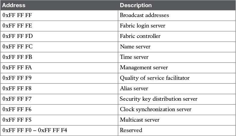
FC-4: ULPs—Application Protocols
The layers FC-0 to FC-3 serve to connect end devices together by means of a Fibre Channel network. However, the type of data that end devices exchange via Fibre Channel connections remains open. This is where the application protocols (upper-layer protocols, or ULPs) come into play. A specific Fibre Channel network can serve as a medium for several application protocols—for example, SCSI and IP.
The task of the FC-4 protocol mappings is to map the application protocols onto the underlying Fibre Channel network. This means that the FC-4 protocol mappings support the application programming interface (API) of existing protocols upward in the direction of the operating system and realize these downward in the direction of the medium via the Fibre Channel network. The protocol mappings determine how the mechanisms of Fibre Channel are used in order to realize the application protocol by means of Fibre Channel. For example, they specify which service classes will be used and how the data flow in the application protocol will be projected onto the exchange sequence frame mechanism of Fibre Channel. This mapping of existing protocols aims to ease the transition to Fibre Channel networks: Ideally, no further modifications are necessary to the operating system except for the installation of a new device driver.
The application protocol for SCSI is called Fibre Channel Protocol (FCP), as shown in Figure 22-31. FCP maps the SCSI protocol onto the underlying Fibre Channel network. For the connection of storage devices to servers, the SCSI cable is therefore replaced by a Fibre Channel network. The idea of the FCP protocol is that the system administrator merely installs a new device driver on the server, and this realizes the FCP protocol. The operating system recognizes storage devices connected via Fibre Channel as SCSI devices, which it addresses like “normal” SCSI devices. This emulation of traditional SCSI devices should make it possible for Fibre Channel SANs to be simply and painlessly integrated into existing hardware and software.

A further application protocol is IPFC, which uses a Fibre Channel connection between two servers as a medium for IP data traffic. IPFC defines how IP packets will be transferred via a Fibre Channel network.
Fibre Connection (FICON) is a further important application protocol. FICON maps the ESCON protocol (Enterprise System Connection) used in the world of mainframes onto Fibre Channel networks. Using ESCON, it has been possible to realize storage networks in the world of mainframes since the 1990s. Fibre Channel is therefore taking the old familiar storage networks from the world of mainframes into the Open System world (UNIX, Windows, OS/400, Novell, and Mac OS).
Fibre Channel—Standard Port Types
Fibre Channel ports are intelligent interface points on the Fibre Channel SAN. They are found embedded in various devices, such as an I/O adapter, array or tape controller, and switched fabric.
When a server or storage device communicates, the interface point acts as the initiator or target for the connection. The server or storage device issues SCSI commands, which the interface point formats to be sent to the target device. These ports understand Fibre Channel. The Fibre Channel switch recognizes which type of device is attaching to the SAN and configures the ports accordingly. Figure 22-32 portrays the various Fibre Channel port types. These port types are detailed in the following list:

![]() Expansion port (E Port): In E Port mode, an interface functions as a fabric expansion port. This port connects to another E Port to create an interswitch link (ISL) between two switches. E Ports carry frames between switches for configuration and fabric management. They also serve as a conduit between switches for frames that are destined to remote node ports (N Ports) and node loop ports (NL Ports). E Ports support Class 2, Class 3, and Class F service.
Expansion port (E Port): In E Port mode, an interface functions as a fabric expansion port. This port connects to another E Port to create an interswitch link (ISL) between two switches. E Ports carry frames between switches for configuration and fabric management. They also serve as a conduit between switches for frames that are destined to remote node ports (N Ports) and node loop ports (NL Ports). E Ports support Class 2, Class 3, and Class F service.
![]() Fabric port (F Port): In F Port mode, an interface functions as a fabric port. This port connects to a peripheral device (such as a host or disk) that operates as an N Port. An F Port can be attached to only one N Port. F Ports support Class 2 and Class 3 service.
Fabric port (F Port): In F Port mode, an interface functions as a fabric port. This port connects to a peripheral device (such as a host or disk) that operates as an N Port. An F Port can be attached to only one N Port. F Ports support Class 2 and Class 3 service.
![]() Fabric loop port (FL Port): In FL Port mode, an interface functions as a fabric loop port. This port connects to one or more NL Ports (including FL Ports in other switches) to form a public FC-AL. If more than one FL Port is detected on the FC-AL during initialization, only one FL Port becomes operational; the other FL Ports enter nonparticipating mode. FL Ports support Class 2 and Class 3 service.
Fabric loop port (FL Port): In FL Port mode, an interface functions as a fabric loop port. This port connects to one or more NL Ports (including FL Ports in other switches) to form a public FC-AL. If more than one FL Port is detected on the FC-AL during initialization, only one FL Port becomes operational; the other FL Ports enter nonparticipating mode. FL Ports support Class 2 and Class 3 service.
![]() Trunking expansion port (TE Port): In TE Port mode, an interface functions as a trunking expansion port. This port connects to another TE Port to create an extended ISL (EISL) between two switches. TE Ports are specific to Cisco MDS 9000 Series switches and expand the functionality of E Ports to support virtual SAN (VSAN) trunking, transport quality of service (QoS) parameters, and the Fibre Channel Traceroute (fctrace) feature. When an interface is in TE Port mode, all frames that are transmitted are in the EISL frame format, which contains VSAN information. Interconnected switches use the VSAN ID to multiplex traffic from one or more VSANs across the same physical link.
Trunking expansion port (TE Port): In TE Port mode, an interface functions as a trunking expansion port. This port connects to another TE Port to create an extended ISL (EISL) between two switches. TE Ports are specific to Cisco MDS 9000 Series switches and expand the functionality of E Ports to support virtual SAN (VSAN) trunking, transport quality of service (QoS) parameters, and the Fibre Channel Traceroute (fctrace) feature. When an interface is in TE Port mode, all frames that are transmitted are in the EISL frame format, which contains VSAN information. Interconnected switches use the VSAN ID to multiplex traffic from one or more VSANs across the same physical link.
![]() Node-proxy port (NP Port): An NP Port is a port on a device that is in N-Port Virtualization (NPV) mode and connects to the core switch via an F Port. NP Ports function like node ports (N Ports) but in addition to providing N Port operations, they also function as proxies for multiple physical N Ports.
Node-proxy port (NP Port): An NP Port is a port on a device that is in N-Port Virtualization (NPV) mode and connects to the core switch via an F Port. NP Ports function like node ports (N Ports) but in addition to providing N Port operations, they also function as proxies for multiple physical N Ports.
![]() Trunking fabric port (TF Port): In TF Port mode, an interface functions as a trunking expansion port. This interface connects to another trunking node port (TN Port) or trunking node-proxy port (TNP Port) to create a link between a core switch and an NPV switch or a host bus adapter (HBA) to carry tagged frames. TF Ports are specific to Cisco MDS 9000 Series switches and expand the functionality of F Ports to support VSAN trunking. In TF Port mode, all frames are transmitted in the EISL frame format, which contains VSAN information.
Trunking fabric port (TF Port): In TF Port mode, an interface functions as a trunking expansion port. This interface connects to another trunking node port (TN Port) or trunking node-proxy port (TNP Port) to create a link between a core switch and an NPV switch or a host bus adapter (HBA) to carry tagged frames. TF Ports are specific to Cisco MDS 9000 Series switches and expand the functionality of F Ports to support VSAN trunking. In TF Port mode, all frames are transmitted in the EISL frame format, which contains VSAN information.
![]() TNP Port: In TNP Port mode, an interface functions as a trunking expansion port. This interface connects to a TF Port to create a link to a core N-Port ID Virtualization (NPIV) switch from an NPV switch to carry tagged frames.
TNP Port: In TNP Port mode, an interface functions as a trunking expansion port. This interface connects to a TF Port to create a link to a core N-Port ID Virtualization (NPIV) switch from an NPV switch to carry tagged frames.
![]() Switched Port Analyzer (SPAN) destination port (SD Port): In SD Port mode, an interface functions as a SPAN. The SPAN feature is specific to Cisco MDS 9000 Series switches. An SD Port monitors network traffic that passes through a Fibre Channel interface. Monitoring is performed using a standard Fibre Channel analyzer (or a similar switch probe) that is attached to the SD Port. SD Ports cannot receive frames and transmit only a copy of the source traffic. This feature is nonintrusive and does not affect switching of network traffic for any SPAN source port.
Switched Port Analyzer (SPAN) destination port (SD Port): In SD Port mode, an interface functions as a SPAN. The SPAN feature is specific to Cisco MDS 9000 Series switches. An SD Port monitors network traffic that passes through a Fibre Channel interface. Monitoring is performed using a standard Fibre Channel analyzer (or a similar switch probe) that is attached to the SD Port. SD Ports cannot receive frames and transmit only a copy of the source traffic. This feature is nonintrusive and does not affect switching of network traffic for any SPAN source port.
![]() SPAN tunnel port (ST Port): In ST Port mode, an interface functions as an entry-point port in the source switch for the Remote SPAN (RSPAN) Fibre Channel tunnel. ST Port mode and the RSPAN feature are specific to Cisco MDS 9000 Series switches. When a port is configured as an ST Port, it cannot be attached to any device and therefore cannot be used for normal Fibre Channel traffic.
SPAN tunnel port (ST Port): In ST Port mode, an interface functions as an entry-point port in the source switch for the Remote SPAN (RSPAN) Fibre Channel tunnel. ST Port mode and the RSPAN feature are specific to Cisco MDS 9000 Series switches. When a port is configured as an ST Port, it cannot be attached to any device and therefore cannot be used for normal Fibre Channel traffic.
![]() Fx Port: An interface that is configured as an Fx Port can operate in either F or FL Port mode. Fx Port mode is determined during interface initialization, depending on the attached N or NL Port.
Fx Port: An interface that is configured as an Fx Port can operate in either F or FL Port mode. Fx Port mode is determined during interface initialization, depending on the attached N or NL Port.
![]() Bridge port (B Port): Whereas E Ports typically interconnect Fibre Channel switches, some SAN extender devices implement a B Port model to connect geographically dispersed fabrics. This model uses B Ports that are as described in the T11 Standard Fibre Channel Backbone 2 (FC-BB-2).
Bridge port (B Port): Whereas E Ports typically interconnect Fibre Channel switches, some SAN extender devices implement a B Port model to connect geographically dispersed fabrics. This model uses B Ports that are as described in the T11 Standard Fibre Channel Backbone 2 (FC-BB-2).
![]() G-Port (Generic_Port): Modern Fibre Channel switches configure their ports automatically. Such ports are called G-Ports. If, for example, a Fibre Channel switch is connected to a further Fibre Channel switch via a G-Port, the G-Port configures itself as an E-Port.
G-Port (Generic_Port): Modern Fibre Channel switches configure their ports automatically. Such ports are called G-Ports. If, for example, a Fibre Channel switch is connected to a further Fibre Channel switch via a G-Port, the G-Port configures itself as an E-Port.
![]() Auto mode: An interface that is configured in auto mode can operate in one of the following modes: F Port, FL Port, E Port, TE Port, or TF Port, with the port mode being determined during interface initialization.
Auto mode: An interface that is configured in auto mode can operate in one of the following modes: F Port, FL Port, E Port, TE Port, or TF Port, with the port mode being determined during interface initialization.
Virtual Storage Area Network
A VSAN is a virtual storage area network (SAN). A SAN is a dedicated network that interconnects hosts and storage devices primarily to exchange SCSI traffic. In SANs, you use the physical links to make these interconnections. A set of protocols runs over the SAN to handle routing, naming, and zoning. You can design multiple SANs with different topologies.
A SAN island refers to a completely physically isolated switch or group of switches used to connect hosts to storage devices. The reasons for building SAN islands include to isolate different applications into their own fabric or to raise availability by minimizing the impact of fabric-wide disruptive events. Figure 22-33 portrays a VSAN topology and a representation of VSANs on an MDS 9700 Director switch by per-port allocation.

Physically separate SAN islands offer a higher degree of security because each physical infrastructure contains a separate set of Cisco Fabric Services and management access. Unfortunately, in practice this situation can become costly and wasteful in terms of fabric ports and resources.
VSANs increase the efficiency of a SAN fabric by alleviating the need to build multiple physically isolated fabrics to meet organizational or application needs. Instead, fewer less-costly redundant fabrics can be built, each housing multiple applications and still providing island-like isolation.
Spare ports within the fabric can be quickly and nondisruptively assigned to existing VSANs, providing a clean method of virtually growing application-specific SAN islands.
VSANs provide not only a hardware-based isolation, but also a complete replicated set of Fibre Channel services for each VSAN. Therefore, when a VSAN is created, a completely separate set of Cisco Fabric Services, configuration management capabilities, and policies are created within the new VSAN.
With the introduction of VSANs, the network administrator can build a single topology containing switches, links, and one or more VSANs. Each VSAN in this topology has the same behavior and properties of a SAN. A VSAN has the following additional features:
![]() Multiple VSANs can share the same physical topology.
Multiple VSANs can share the same physical topology.
![]() The same Fibre Channel IDs (FC IDs) can be assigned to a host in another VSAN, thus increasing VSAN scalability.
The same Fibre Channel IDs (FC IDs) can be assigned to a host in another VSAN, thus increasing VSAN scalability.
![]() Every instance of a VSAN runs all required protocols, such as FSPF, domain manager, and zoning.
Every instance of a VSAN runs all required protocols, such as FSPF, domain manager, and zoning.
![]() Fabric-related configurations in one VSAN do not affect the associated traffic in another VSAN.
Fabric-related configurations in one VSAN do not affect the associated traffic in another VSAN.
![]() Events causing traffic disruptions in one VSAN are contained within that VSAN and are not propagated to other VSANs.
Events causing traffic disruptions in one VSAN are contained within that VSAN and are not propagated to other VSANs.
Using a hardware-based frame tagging mechanism on VSAN member ports and EISL links isolates each separate virtual fabric. The EISL link type has been created and includes added tagging information for each frame within the fabric. The EISL link is supported between Cisco MDS and Nexus switch products. Membership to a VSAN is based on physical ports, and no physical port may belong to more than one VSAN.
VSANs offer the following advantages:
![]() Traffic isolation: Traffic is contained within VSAN boundaries, and devices reside in only one VSAN, ensuring absolute separation between user groups, if desired.
Traffic isolation: Traffic is contained within VSAN boundaries, and devices reside in only one VSAN, ensuring absolute separation between user groups, if desired.
![]() Scalability: VSANs are overlaid on top of a single physical fabric. The ability to create several logical VSAN layers increases the scalability of the SAN.
Scalability: VSANs are overlaid on top of a single physical fabric. The ability to create several logical VSAN layers increases the scalability of the SAN.
![]() Per VSAN fabric services: Replication of fabric services on a per-VSAN basis provides increased scalability and availability.
Per VSAN fabric services: Replication of fabric services on a per-VSAN basis provides increased scalability and availability.
![]() Redundancy: Several VSANs created on the same physical SAN ensure redundancy. If one VSAN fails, redundant protection (to another VSAN in the same physical SAN) is configured using a backup path between the host and the device.
Redundancy: Several VSANs created on the same physical SAN ensure redundancy. If one VSAN fails, redundant protection (to another VSAN in the same physical SAN) is configured using a backup path between the host and the device.
![]() Ease of configuration: Users can be added, moved, or changed between VSANs without changing the physical structure of a SAN. Moving a device from one VSAN to another only requires configuration at the port level, not at a physical level.
Ease of configuration: Users can be added, moved, or changed between VSANs without changing the physical structure of a SAN. Moving a device from one VSAN to another only requires configuration at the port level, not at a physical level.
Up to 256 VSANs can be configured in a switch. Of these, one is a default VSAN (VSAN 1) and another is an isolated VSAN (VSAN 4094). User-specified VSAN IDs range from 2 to 4093. Different characteristics of a VSAN can be summarized as below:
![]() VSANs equal SANs with routing, naming, and zoning protocols.
VSANs equal SANs with routing, naming, and zoning protocols.
![]() VSANs limit unicast, multicast, and broadcast traffic.
VSANs limit unicast, multicast, and broadcast traffic.
![]() Membership is typically defined using the VSAN ID to Fx ports.
Membership is typically defined using the VSAN ID to Fx ports.
![]() An HBA or a storage device can belong only to a single VSAN—the VSAN associated with the Fx port.
An HBA or a storage device can belong only to a single VSAN—the VSAN associated with the Fx port.
![]() VSANs enforce membership at each E port, source port, and destination port.
VSANs enforce membership at each E port, source port, and destination port.
![]() VSANs are defined for larger environments (storage service providers).
VSANs are defined for larger environments (storage service providers).
![]() VSANs encompass the entire fabric.
VSANs encompass the entire fabric.
![]() VSANs equal SANs with routing, naming, and zoning protocols. Dynamic Port VSAN Membership (DPVM).
VSANs equal SANs with routing, naming, and zoning protocols. Dynamic Port VSAN Membership (DPVM).
Port VSAN membership on the switch is assigned on a port-by-port basis. By default, each port belongs to the default VSAN. You can dynamically assign VSAN membership to ports by assigning VSANs based on the device WWN. This method is referred to as Dynamic Port VSAN Membership (DPVM). DPVM offers flexibility and eliminates the need to reconfigure the port VSAN membership to maintain fabric topology when a host or storage device connection is moved between two Cisco MDS switches or two ports within a switch. It retains the configured VSAN regardless of where a device is connected or moved.
DPVM configurations are based on port World Wide Name (pWWN) and node World Wide Name (nWWN) assignments. A DPVM database contains mapping information for each device pWWN/nWWN assignment and the corresponding VSAN. The Cisco NX-OS software checks the database during a device FLOGI and obtains the required VSAN details.
The pWWN identifies the host or device, and the nWWN identifies a node consisting of multiple devices. You can assign any one of these identifiers or any combination of these identifiers to configure DPVM mapping. If you assign a combination, preference is given to the pWWN. DPVM uses the Cisco Fabric Services (CFS) infrastructure to allow efficient database management and distribution.
Inter-VSAN Routing (IVR)
Virtual SANs (VSANs) improve storage area network (SAN) scalability, availability, and security by allowing multiple Fibre Channel SANs to share a common physical infrastructure of switches and ISLs. These benefits are derived from the separation of Fibre Channel services in each VSAN and the isolation of traffic between VSANs (see Figure 22-34). Data traffic isolation between the VSANs also inherently prevents sharing of resources attached to a VSAN, such as robotic tape libraries. Using IVR, you can access resources across VSANs without compromising other VSAN benefits. IVR transports data traffic between specific initiators and targets on different VSANs without merging VSANs into a single logical fabric. It establishes proper interconnected routes that traverse one or more VSANs across multiple switches. IVR is not limited to VSANs present on a common switch. Fibre Channel traffic does not flow between VSANs, nor can initiators access resources across VSANs other than the designated VSAN. It provides efficient business continuity or disaster recovery solutions when used in conjunction with Fibre Channel over IP (FCIP).

Internet Small Computer System Interface (iSCSI)
IP and Small Computer System Interface over IP (iSCSI) storage refer to the block access of storage disks across devices connected using traditional Ethernet and TCP/IP networks. iSCSI is an IP-based storage networking standard for linking data storage facilities.
The iSCSI protocol enables transport of SCSI commands over TCP/IP networks. By transmitting SCSI commands over IP networks, iSCSI can facilitate block-level transfers over an intranet and the Internet. The iSCSI architecture is similar to a client-server architecture in which the client initiates an I/O request to the storage target. The TCP payload of an iSCSI packet contains iSCSI protocol data units (PDUs), all of which begin with one or more header segments followed by zero or more data segments. iSCSI uses TCP (typically TCP ports 860 and 3260) for the protocols itself, with higher-level names used to address the objects within the protocol.
iSCSI Terminology
An iSCSI network consists of multiple devices such as iSCSI initiators and iSCSI targets. Each device has various components associated with it. Some of the iSCSI components that make up an iSCSI storage network are listed here:
![]() iSCSI name: The iSCSI name is a unique World Wide Name (WWN) by which the iSCSI node is known. The iSCSI name uses one of the following formats:
iSCSI name: The iSCSI name is a unique World Wide Name (WWN) by which the iSCSI node is known. The iSCSI name uses one of the following formats:
![]() iSCSI qualified name (IQN): For example, iqn.1987-05.com.Cisco.00.9f9ccf185aa3508c.taget2
iSCSI qualified name (IQN): For example, iqn.1987-05.com.Cisco.00.9f9ccf185aa3508c.taget2
Format: The iSCSI qualified name is documented in RFC 3720, with further examples of names in RFC 3721. Briefly, the fields are as follows:
Literal iqn (iSCSI qualified name)
Date (yyyy-mm) that the naming authority took ownership of the domain
Reversed domain name of the authority
Optional “:” prefixing a storage target name specified by the naming authority.
![]() Extended unique identifier (EUI-64 bit addressing): Format: eui.02004565A425678D.
Extended unique identifier (EUI-64 bit addressing): Format: eui.02004565A425678D.
![]() T11 Network Address Authority (NAA): IQN format addresses occur most commonly. They are qualified by a date (yyyy-mm) because domain names can expire or be acquired by another entity. Format: naa.{NAA 64 or 128 bit identifier} (for example, naa.52004567BA64678D).
T11 Network Address Authority (NAA): IQN format addresses occur most commonly. They are qualified by a date (yyyy-mm) because domain names can expire or be acquired by another entity. Format: naa.{NAA 64 or 128 bit identifier} (for example, naa.52004567BA64678D).
![]() iSCSI node: The iSCSI node represents a single iSCSI initiator or iSCSI target.
iSCSI node: The iSCSI node represents a single iSCSI initiator or iSCSI target.
![]() Network entity: The network entity represents a device or gateway that is accessible from the IP network (for example, a host or storage array).
Network entity: The network entity represents a device or gateway that is accessible from the IP network (for example, a host or storage array).
![]() Network portal: The network portal is a component of a network entity that has a TCP/IP network address that is used by an iSCSI node. A network portal in an initiator is identified by its IP address, and a target is identified by its IP address and its listening TCP port.
Network portal: The network portal is a component of a network entity that has a TCP/IP network address that is used by an iSCSI node. A network portal in an initiator is identified by its IP address, and a target is identified by its IP address and its listening TCP port.
A network entity contains one or more iSCSI nodes. The iSCSI node is accessible through one or more network portals. An iSCSI node is identified by its iSCSI name. Figure 22-35 shows the components of an iSCSI network.
An initiator functions as an iSCSI client. An initiator typically serves the same purpose to a computer as a SCSI bus adapter would, except that, instead of physically cabling SCSI devices (such as hard drives and tape changers), an iSCSI initiator sends SCSI commands over an IP network. An initiator falls into two broad types: a software initiator and hardware initiator.
A software initiator uses code to implement iSCSI. Typically, this happens in a kernel-resident device driver that uses the existing network card (NIC) and network stack to emulate SCSI devices for a computer by speaking the iSCSI protocol. Software initiators are available for most popular operating systems and are the most common method of deploying iSCSI.

A hardware initiator uses dedicated hardware, typically in combination with firmware running on that hardware, to implement iSCSI. A hardware initiator mitigates the overhead of iSCSI and TCP processing and Ethernet interrupts, and thus may improve the performance of servers that use iSCSI. An iSCSI host bus adapter (HBA) implements a hardware initiator. A typical HBA is packaged as a combination of a Gigabit (or 10 Gigabit) Ethernet network interface controller, some kind of TCP/IP offload engine (TOE) technology, and a SCSI bus adapter, which is how it appears to the operating system. An iSCSI HBA can include PCI option ROM to allow booting from an iSCSI SAN.
An iSCSI offload engine, or iSOE card, offers an alternative to a full iSCSI HBA. An iSOE “offloads” the iSCSI initiator operations for this particular network interface from the host processor, freeing up CPU cycles for the main host applications. iSCSI HBAs or iSOEs are used when the additional performance enhancement justifies the additional expense of using an HBA for iSCSI, rather than using a software-based iSCSI client (initiator). iSOE may be implemented with additional services such as TCP offload engine (TOE) to further reduce host server CPU usage.
The iSCSI specification refers to a storage resource located on an iSCSI server (more generally, one of potentially many instances of iSCSI storage nodes running on that server) as a target.
The term “iSCSI target” should not be confused with the term “iSCSI,” because the latter is a protocol and not a storage server instance.
An iSCSI target is often a dedicated network-connected hard disk storage device, but may also be a general-purpose computer, because as with initiators, software to provide an iSCSI target is available for most mainstream operating systems.
iSCSI Session
The highest level target available for most mainstream operating systems of an iSCSI communications path is a session that is formed between an iSCSI initiator and an iSCSI target. Two types of sessions are defined in iSCSI:
![]() An iSCSI discovery and login session used by the initiator to discover available targets
An iSCSI discovery and login session used by the initiator to discover available targets
![]() A general iSCSI session to transfer SCSI data and commands after the login
A general iSCSI session to transfer SCSI data and commands after the login
A session is identified by a session ID (SSID), which consists of initiator (ISID) and target (TSID) components. TCP connections can be added and removed within a session; however, all connections are between the same unique initiator and target iSCSI nodes. Each connection within a session has a unique connection ID (CID).
An iSCSI session is established through the iSCSI login process. This session is used to identify all TCP connections associated with a particular SCSI initiator and target pair. One session can contain one or more TCP connections. The login process is started when the initiator establishes a TCP connection to the desired target either through the well-known port (3260) or a specified target port. The initiator and target can authenticate each other and negotiate a security protocol. During the login phase, numerous attributes are negotiated between the iSCSI initiator and target. Upon successful completion of the login phase, the session enters the full-featured phase.
Reference List
Storage Network Industry Association (SNIA)—http://www.snia.org
Internet Engineering Task Force – IP Storage— https://datatracker.ietf.org/wg/ips/documents/
ANSI T11 – Fibre Channel—http://www.t11.org/index.html
ANSI T10 Technical Committee—www.T10.org
IEEE Standards site—http://standards.ieee.org
SNIA dictionary—http://www.snia.org/education/dictionary
Farley, Marc. Rethinking Enterprise Storage: A Hybrid Cloud Mode. Microsoft Press, 2013
Kembel, Robert W. Fibre Channel: A Comprehensive Introduction. Northwest Learning Associates, Inc., 2000
Exam Preparation Tasks
Review All Key Topics
Review the most important topics in the chapter, noted with the key topics icon in the outer margin of the page. Table 22-10 lists a reference for these key topics and the page numbers on which each is found.


Complete Tables and Lists from Memory
Print a copy of Appendix C, “Memory Tables,” or at least the section for this chapter, and complete the tables and lists from memory. Appendix D, “Memory Tables Answer Key,” includes completed tables and lists to check your work.
Define Key Terms
Define the following key terms from this chapter, and check your answers in the glossary:
virtual storage-area network (VSAN)
zoning
fan-out ratio
fan-in ratio
logical unit number (LUN) masking
LUN mapping
Extended Link Services (ELS)
multipathing
Big Data
IoE
N_Port Login (PLOGI)
F_Port Login (FLOGI)
logout (LOGO)
process login (PRLI)
process logout (PRLO)
state change notification (SCN)
registered state change notification (RSCN)
state change registration (SCR)
inter-VSAN routing (IVR)
Fibre Channel Generic Services (FC-GS)
hard disk drive (HDD)
solid-state drive (SSD)
Small Computer System Interface (SCSI)
initiator
target
American National Standards Institute (ANSI)
International Committee for Information Technology Standards (INCITS)
Fibre Connection (FICON)
T11
Input/output Operations per Second (IOPS)
Common Internet File System (CIFS)
Network File System (NFS)
Cisco Fabric Services (CFS)
Top-of-Rack (ToR)
End-of-Row (EoR)
Dynamic Port VSAN Membership (DPVM)
inter-VSAN routing (IVR)