
In Appendix A the strength-of-materials theory of the truncated semi-infinite cone [M5, M11] is derived. This one-sided cone is used directly to model a disk on the surface of a homogeneous soil halfspace, or as a double-cone model represents a disk embedded in a fullspace. The trapped mass present for incompressible material for the vertical and rocking motions (see Section 2.1.4) can be shifted to the basemat and thus to the superstructure. This “trick” enables the analysis of the cone models in the same manner for all values of Poisson’s ratio. Section A1 addresses the translational cone, whereby axial distortion (vertical motion) is examined; for the distortion in shear (horizontal motion) the derivation is analogous. Based on the equation of motion of rod (bar) theory, the interaction force-displacement relationship of the disk in the truncated cross section of the cone used in the stiffness formulation is developed, followed by the corresponding displacement-interaction force equation applied in the flexibility formulation. The Green’s function is then discussed, the displacement along the axis of the cone caused by a unit impulse force acting on the disk. In Section A2 the same derivations are performed for the rotational cone. Again, rotational axial distortion corresponding to the rocking motion is addressed, but the results are also valid for rotational shear distortion as in torsional motion. All developments are first performed in the time domain and then, if used in the text, repeated for a harmonic load (frequency domain).
Section A3 examines the generalized wave pattern [M6] for the unfolded layered cone used to model a disk foundation on the surface of a soil layer.
The translational truncated semi-infinite cone with the apex height z0 and the radius r0 is shown for axial distortion in Fig. A-1, which is used to model the vertical degree of freedom of a disk of radius r0 on the surface of a halfspace. The area A at depth z equals ![]() A0 with
A0 with ![]() , where z is measured from the apex. With c denoting the appropriate wave velocity of the compression-extension waves (dilatational waves) and ρ the mass density, ρ c2 is equal to the corresponding elastic modulus (constrained modulus). Also, u represents the axial displacement and N the axial force. Radial effects are disregarded. Formulating the equilibrium equation of an infinitesimal element (Fig. A-1) taking the inertial loads into account,
, where z is measured from the apex. With c denoting the appropriate wave velocity of the compression-extension waves (dilatational waves) and ρ the mass density, ρ c2 is equal to the corresponding elastic modulus (constrained modulus). Also, u represents the axial displacement and N the axial force. Radial effects are disregarded. Formulating the equilibrium equation of an infinitesimal element (Fig. A-1) taking the inertial loads into account,
and substituting the force-displacement relationship,
leads to the equation of motion in the time domain of the translational cone
which may be rewritten as a one-dimensional wave equation in zu
The familiar solution of the wave equation in the time domain is
where f and g are arbitrary functions of the argument for outward-propagating (in the positive z-direction) and inward-propagating waves (in the negative z-direction), respectively.

In a radiation problem only outward-propagating waves are permissible (g = 0).
For harmonic loading of frequency ω resulting in the response u(t) = u(ω)eiωt, substituting ![]() in Eq. A-4 leads to the wave equation in zu(ω) with the displacement amplitude u(ω)
in Eq. A-4 leads to the wave equation in zu(ω) with the displacement amplitude u(ω)
The solution omitting the inward-propagating wave varying as e+iω(z-z0)c equals
with the integration constant c1.
For a prescribed displacement u0 of the disk, the interaction force P0 is calculated as follows. Enforcing the boundary condition u(z = z0) = u0 yields from Eq. A-6
and thus the displacement decays in inverse proportion to the depth z
With
where ![]() denotes differentiation of u0 with respect to the argument t–(z – z0)/c.
denotes differentiation of u0 with respect to the argument t–(z – z0)/c.
is rewritten as ![]()
or
In this interaction force-displacement relationship K and C are the constant coefficients of the spring and dashpot:
or
applies with the dynamic-stiffness coefficient S(ω)
Introducing the dimensionless frequency parameter b0 defined with respect to the properties of the cone
S(ω) is formulated as
with the (dimensionless) spring and damping coefficients being independent of b0 in this simple case
For a prescribed interaction force P0 acting on the disk, the displacement u0 is determined as follows. Dividing Eq. A-13 by K (Eq. A-15a) leads to the first-order differential equation in u0
The general solution is the convolution integral
with the unit-impulse response function
Equation A-23 derived purely on mathematical grounds can be interpreted physically as follows. The contribution of the infinitesimal pulse (1/K)P0(τ) dτ acting at time τ to the displacement du0(t) at time t (t > τ) depends on the unit-impulse response function evaluated for the time difference t – τ, h1(t – τ)
The displacement-interaction force relationship (Eq. A-23) is the integral of Eq. A-25 over all pulses from 0 < τ < t.
For harmonic loading, the dynamic-flexibility coefficient F(ω) follows from Eqs. A-17 and A-18 through inversion:
with
or using Eqs A-16, A-15 and A-19
The unit-impulse response function (1/K) h1(t) and the dynamic-flexibility coefficient F(ω) form a Fourier-transform pair.
The Green’s function in the time domain is defined as the displacement as a function of time u(t) at a point, called the receiver, located at a distance a from the disk, the source (Fig. A-1), which is excited at time = 0 by a unit-impulse force P0. The motion of the receiver at time t will have originated earlier at the source, at the retarded time t – a/c, with c = the appropriate wave velocity. Furthermore, the amplitude will have diminished after traveling the distance a. Thus the Green’s function may be denoted as u(t) = g (a, t – a/c). The first argument specifies the spatial distance from the source, the second argument the appropriate retarded time at the source.
Applying a unit-impulse force P0(τ) = δ(τ) (with δ(τ) denoting the Dirac-delta function) at time τ = 0,
follows from Eq. A-23, as ![]() . Enforcing the boundary condition u0 = u (z = z0) yields from Eq. A-6
. Enforcing the boundary condition u0 = u (z = z0) yields from Eq. A-6
Replacing u by g(a, t – a/c) and with a = z – z0 leads to
or after substituting Eq. A-24 the Green’s function equals

For harmonic loading, the displacement amplitude u0(ω) caused by a unit interaction force amplitude P0(ω) = 1 follows from Eq. A-26 as
Enforcing the boundary condition u0(ω) = u(z = z0, ω) in Eq. A-8 leads to
Replacing u(ω) by g(a, ω) results in
or, after substituting Eq. A-28, the Green’s function equals

The factor e-iωa/c) arises from the time lag a/c. And g(a, ω) can be rewritten as

where
The Fourier transform of H1(ω) is h1(t). Introducing the dynamic-stiffness coefficient S(ω) specified in Eqs. A-20 and A-21,

follows.
As g(a, t – a/c) and g(a, ω) form a Fourier-transform pair, the Green’s function in the time domain can also be calculated as
The Green’s functions calculated above correspond to the one-sided cone. For the double-cone model used in the dynamic analysis of embedded and pile foundations, the right-hand sides are multiplied by 0.5, as K in Eqs. A-33 and A-37; A-38 is replaced by 2K.
The rotational truncated semi-infinite cone is presented for rotational axial distortion in Fig. A-2. This model is used to represent the rocking degree of freedom of a disk on the surface of a halfspace. With ![]() the moment of inertia I at depth z equals
the moment of inertia I at depth z equals ![]() . Also V denotes the rotation and M the bending moment. Formulating the equilibrium equation of an infinitesimal element
. Also V denotes the rotation and M the bending moment. Formulating the equilibrium equation of an infinitesimal element
and substituting the moment-rotation relationship
results in the equation of motion in the time domain of the rotational cone
Introducing a dimensionless potential function φ such that
which when substituted in Eq. A-44 leads to

or

The equivalence of the previous two equations may be verified by expanding the derivatives of Eq. A-47. A solution is apparent by inspection
The left-hand side is recognized as the wave equation in z φ. It turns out to be convenient to specify the constant on the right-hand side to be ![]() . Then the solution of this modified wave equation takes the form
. Then the solution of this modified wave equation takes the form
with additional constants of integration Φ and F. The minus sign preceding the term in brackets is chosen for convenience. As for the translational cone, V1(t – (z – z0)/c) is any arbitrary function of the argument for outward-propagating waves. Inward-propagating waves are thus omitted. The correctness of the solution is verified by insertion of Eq. A-49 into Eq. A-48. Note that F is nothing more than a constant shift and may be incorporated into V1(t – (z – z0)/c). With this simplification the potential function becomes
The angle of rotation V is retrieved via Eq. A-45
where ![]() represents differentiation with respect to the argument t – (z – z0)/c. Without loss of generality the constant shift Θ may be incorporated into V (i.e., set equal to zero), resulting in
represents differentiation with respect to the argument t – (z – z0)/c. Without loss of generality the constant shift Θ may be incorporated into V (i.e., set equal to zero), resulting in
This solution with outward-propagating waves for the rotational cone can be compared to that for the translational cone in Eq. A-6.
For harmonic motion the equation of motion corresponding to Eq. A-44 equals
The solution with outward-propagating waves is written as
For a specified rotation V0 of the disk, the variation of the angle of rotation V with z and the interaction moment M0 are calculated as follows. Enforcing the boundary condition V (z = z0) = V0 yields from Eq. A-52
where at ![]() . The general solution of this first-order differential equation is the convolution
. The general solution of this first-order differential equation is the convolution
with the unit-impulse response function h1(t) defined in Eq. A-24. Formulating Eq. A-55 with the argument t – (z – z0)/c instead of t and thus ![]() instead of
instead of ![]() , which corresponds to a time shift, allows
, which corresponds to a time shift, allows ![]() to be eliminated from Eq. A-52, leading to
to be eliminated from Eq. A-52, leading to
At the surface (z = z0) the contribution of the second term vanishes and V(z = z0) = V0. In the underground region, however, part of the rotation is due to the convolution V1; and the amplitude decays in inverse proportion to a combination of the square and the cube of depth z.
Two limiting cases are of particular interest. For static loading (V0 = constant), V1 = V0 (Eq. A-55), which yields from Eq. A-57 the static limit
On the other hand, for high-frequency harmonic motion the convolution V1 tends to zero (as is verified from Eq. A-55) and Eq. A-57 reverts to the high-frequency limit
Turning to M0, the derivative Vz is calculated via the chain rule from Eq. A-52
At z = z0, with V0,z = Vz(z = z0)
applies. Using Eq. A-55, the first two terms on the right-hand side are equal to –3/z0 V0. To eliminate ![]() Eq. A-55 is differentiated with respect to time
Eq. A-55 is differentiated with respect to time
This first-order differential equation in ![]() can be solved as
can be solved as
Substituting for ![]() , from Eqs. A-62 in Eq. A-61 and then eliminating
, from Eqs. A-62 in Eq. A-61 and then eliminating ![]() using Eq. A-63 leads to
using Eq. A-63 leads to
Finally, with
the interaction moment-rotation relationship is formulated as
or
Kv and Cv are the constant coefficients of the rotational spring and dashpot
The convolution which is preceded by a negative sign with h1 specified in Eq. A-24 involves the rotational velocity ![]() , which leads to the rotational static-stiffness coefficient Kv appearing in the interaction moment-rotation relationship. If the convolution is performed with the rotation V0,
, which leads to the rotational static-stiffness coefficient Kv appearing in the interaction moment-rotation relationship. If the convolution is performed with the rotation V0,
is derived. This form is not attractive because of the factor 2/3 with which the static-stiffness coefficient is multiplied to form the spring coefficient.
For harmonic loading, enforcing the boundary condition V0(ω) = V(z = z0, ω) yields the integration constant c1 in Eq. A-54. The rotational amplitude with depth z follows as

The equation
leads with b0 defined in Eq. A-19 to
where the dynamic-stiffness coefficient
with
For a prescribed interaction moment M0 acting on the disk, the rotation V0 is calculated as follows. Enforcing the boundary condition (Eq. A-65) and substituting Eq. A-61 leads to
To derive the unit-impulse response function h2(t) for the rotation V0, the loading M0/Kv is equal to the Dirac-delta function δ(t).
The solution of this second-order differential equation can be derived by noting that the latter has the same form as the dynamic equation of motion of a one-degree-of-freedom system with viscous damping.
The unit-impulse response function h(t) is equal to the damped vibration for an initial velocity δ(t)dt/m = 1/m
with the natural frequency ω0, the damping ratio ζ, and the damped frequency ωd
From Eq. A-78, V1(t) follows. Comparing Eq. A-77 to Eq. A-76,
Substituting in Eq. A-52 for z = z0, the unit-impulse response function h2(t) which is equal to V0(t) is written as
The rotation-interaction moment relationship is specified as the convolution integral (Eq. A-75)
For harmonic loading, the dynamic-flexibility coefficient Fv(ω) follows from Eq. A-72 through inversion
In Eq. A-19 b0 is defined. As (1/Kv) h2(t) and Fv(ω) form a Fourier-transform pair, h2(t) can also be determined as
Exciting the disk, the source, at time t = 0 by a unit-impulse moment M0, the rotation as a function of time V(t) at the receiver, located at a distance a from the source (Fig. A-2), is equal to the Green’s function gv (a, t – a/c). As for the translational cone (Section A1.4), the Green’s function is a function of a which governs the attenuation of the wave and of the retarded time t – a/c.
Applying a unit-impulse moment M0(τ) = δ(τ), the rotation of the disk V0 determined from Eq. A-82 equals
The equation of V(z, t) specified in Eq. A-52 leads after enforcing the boundary condition V0 = V(z = z0) to the first-order differential equation in V1(t) (Eq. A-55) with the solution given in Eq. A-56. Substituting Eq. A-86 into this equation yields
Another unit-impulse response function, h3(t), is defined as
with, after substituting h1(t) from Eq. A-24 and h2(t) from Eq. A-81,
Substituting Eq. A-87 with Eq. A-88 and Eq. A-86 in Eq. A-57 and replacing V with gv (a, t – a/c) and with a = z – z0 leads to the Green’s function

Both h2(t – a/c) and h3(t – a/c) are specified in Eqs. A-81 and A-89 with t replaced by t – a/c.
For harmonic loading, the rotation amplitude V0(ω) caused by a unit interaction moment amplitude M0(ω) = 1 follows from Eq. A-83 as
Enforcing this boundary condition V0(ω) = V(z = z0, ω) in Eq. A-54 yields
Replacing V(ω) by gv(a, ω) results in

or after substituting Eq. A-84 the Green’s function equals

Here e-iωa/c represents the time-lag factor. Thus, gv(a,ω) can be rewritten as

where


The Fourier transforms of H2(ω) and H3(ω) are h2(t) and h3(t), respectively. Introducing the dynamic-stiffness coefficient Sv(ω) specified in Eqs. A-73 and A-74 results in

Again, as g(a, t – a/c) and gv(a,ω) form a Fourier-transform pair, the Green’s function in the time domain can also be determined as
The Green’s functions specified above correspond to the one-sided cone. For the double-cone model used in the dynamic analysis of embedded and pile foundations, the right-hand sides are multiplied by 0.5, as Kv in Eqs. A-90 and A-94, A-95, A-98 is replaced by 2Kv.
As discussed in Section 3.1, a generalized wave pattern w(z, t) may be postulated for an unfolded layered cone, in which the amplitude of motion decays in inverse proportion to the Mh power of the distance from the apex:

The barred time history ![]() ) generates the motion. For the unfolded layered cone in rotation, there are three such
) generates the motion. For the unfolded layered cone in rotation, there are three such ![]() functions. The first corresponds to
functions. The first corresponds to ![]() with N = 2; the second corresponds to
with N = 2; the second corresponds to ![]() with N = 3; and the third corresponds to
with N = 3; and the third corresponds to ![]() , with N = 2. Since they superpose independently, attention may be restricted to any one of these three separate generating functions. To verify Eq. A-100, it suffices to consider the first few terms of the sum:
, with N = 2. Since they superpose independently, attention may be restricted to any one of these three separate generating functions. To verify Eq. A-100, it suffices to consider the first few terms of the sum:

The displacement wd at bedrock (z = d) is
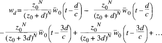
Since the terms cancel pair-for-pair, the displacement wd at bedrock is zero; that is, the layer is, as it should be, built-in at its base.
The strain is equal to the spatial derivative of w. Application of the chain rule to Eq. A-101 yields

In this expression ![]() denotes differentiation with respect to the complete argument of the generating function, that is
denotes differentiation with respect to the complete argument of the generating function, that is ![]() with for example ( ) = t – 2d/c + z/c. The strain at the surface (z = 0) is
with for example ( ) = t – 2d/c + z/c. The strain at the surface (z = 0) is

in which the ![]() derivatives revert to the velocity
derivatives revert to the velocity ![]() . Due to the free-surface boundary condition implicit in Eq. A-104, the strain contributions resulting from the reflected waves cancel pair-for-pair. The strain at the surface (first two terms in Eq. A-104) is identical to that of an unlayered cone subjected to the generating motion
. Due to the free-surface boundary condition implicit in Eq. A-104, the strain contributions resulting from the reflected waves cancel pair-for-pair. The strain at the surface (first two terms in Eq. A-104) is identical to that of an unlayered cone subjected to the generating motion ![]() and
and ![]() .
.
The relationship between the generating motion ![]() of the associated unlayered cone and the true surface motion w0 of the unfolded layered cone is found by evaluating Eq. A-100 at the surface (z = 0):
of the associated unlayered cone and the true surface motion w0 of the unfolded layered cone is found by evaluating Eq. A-100 at the surface (z = 0):
with echo interval T = 2d/c and geometric parameter κ = 2d/z0. Introducing echo constants ![]() allows Eq. A-105 to be expressed concisely as
allows Eq. A-105 to be expressed concisely as
with
and for; j ≥ 1
For the rotational cone the various contributions associated with N = 2 and N = 3 are simply superposed to determine V0(t).