
Driving Around Town
Optimizing A Real-World Code Example
Now that we have taken our sports car on the open road and experienced some easier-to-navigate challenges, we will increase the difficulty and deal with some real-world circumstances, similar to what might be experienced in general driving around a city or town. To drive around town to someplace like the grocery store, you must navigate through intersections, stop signs, traffic signals, and sometimes unexpected detours. Rules of the road constrain your speed and direction. Changing circumstances require using the information at hand, and the knowledge of how the car will respond to drive safely and most efficiently to your destination.

In this chapter, we will extend our sports car analogy to a real scientific code example that comes from Naoya Maruyama of Riken Advanced Institute for Computational Science in Japan. The purpose of the code is to simulate diffusion of a solute through a volume of liquid over time within a 3D container such as a cube, as depicted in Figure 4.1. A three-dimensional seven-point stencil operation is used to calculate the effects on the neighboring sub-volume sections on each other over time. So, if there is no food on our shelves, we need to head out to the street and learn the best paths get to the grocery store as quickly as we can!

Figure 4.1 Diffusion of a Compound over Time through an Enclosed Volume.
Choosing the direction: the basic diffusion calculation
Before we start driving on the road, we should know which direction goes towards our destination. Similarly, we need to understand enough about the algorithm being used to ensure we perform correct and complete calculations. A shown in Figure 4.2, we are going to apply a seven-point stencil to calculate a new density in the volume using weighted values in the stencil applied to the current target sub-volume and its neighbors.

Figure 4.2 3D Stencil Used to Calculate the Diffusion of a Solute through a Liquid Volume.
We will repeat this calculation for every section of the volume creating a new baseline volume. The code then iterates over the number of time steps selected to create the final diffused volume state.
The baseline C code that shows the primary diffusion algorithm implementation is shown in Figure 4.3. The f1[] array contains the current volume data and the f2[] array is used to store the results of the current time step iteration. Four loops, one for each dimension and one for the number of time steps requested, are implemented. The inner loop applies the stencil calculations using the target center sub-volume section and its neighboring north, south, east, west, top, and bottom sections. Once all the sub-volumes for the current time step are processed, the f1[] and f2[] array pointers are swapped, setting the new reference state. While easy to read, this implementation is equivalent to a straight road with no turns available; it will not take us to our desired destination.

Figure 4.3 Baseline Stencil Diffusion Algorithm Code, No Consideration for Boundary Conditions.
Turn ahead: accounting for boundary effects
Like approaching a T intersection where we must make a turn or drive off the road, we must account for a structural issue with our diffusion simulation; the three-dimensional container has boundary walls. Since our stencil operates on each sub-volume section that comprises the whole, we need to consider how to properly calculate the molecular density for sub-volumes that sit next to the edges of our container. At a minimum, we need to avoid calculating array index values that go outside our allocated memory space representing the volume.
Figure 4.4 shows an evolved implementation that accounts for the boundary conditions. The implementation also simplifies the f1[] array access by linearizing the stencil indices by adding the w, e, n, s, b, t (west, east, north, south, bottom, top) variables. The boundary conditions occur for any sub-volume that has an x, y, or z value of zero or x, y, or z value at the full width, height, or depth of the volume as represented by the variables nx, ny, and nz. In these cases, we simply replace the value of the neighbor volume with the target central density value to get a reasonable approximation of the diffusion at that point. Now, we have reached the first important stage of implementing a real-world algorithm; it will provide the complete and correct results when run.

Figure 4.4 Working Diffusion Calculation with Boundary Processing.
Figure 4.5 shows the complete code listing. The function diffusion_baseline() implements the key computational processing.
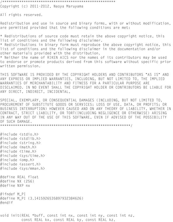
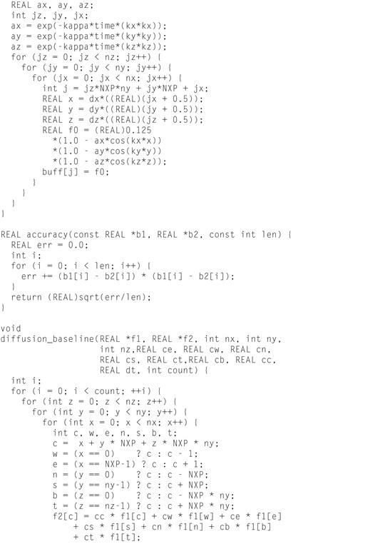
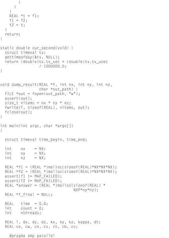

Figure 4.5 The diffusion_baseline.c Listing.
Looking at the main() function, we see that two arrays of equal size, f1[] and f2[], are allocated to support the double buffering used in the primary calculation function. The double buffering is required to ensure the stencil processing is completed without modifying the in-place target volume data, which will be used in subsequent calculations when its neighboring sub-volumes are calculated.
After initializing that f1[] array, and the east, west, north, south, top, bottom, stencil diffusion weights, ce, cw, cn, cs, ct, cb, and the time step dt, based on the size of the volume, the time step is used to determine the iteration count. Next, a time stamp is taken and the diffusion calculation function is called to perform count time steps. Upon completion of the function, the resulting floating-point performance is calculated based on the thirteen floating-point operations per inner loop iteration, and the memory bandwidth (in GB/s) is determined, using number of bytes of volume data read and written during the call.
Since we have not applied any optimizations, such as scaling across cores, when compiled and run we can expect this single-threaded code to perform quite slowly. If you take our word for it, you can skip compiling and running this baseline code yourself; it will indeed take well over an hour for the run to complete. You will have several more opportunities to follow along and study the improvements where the code runs much faster. However, to establish an initial baseline performance we will show you our results as below.
To compile the code to run natively on the Intel® Xeon Phi™ coprocessor use the following command:
$ icc –openmp –mmic –std=c99 –O3 –vect-report=3 diffusion_base.c -0 diffusion_base
Upload the executable program diffusion_base to the coprocessor and then on the coprocessor command prompt in your working directory execute the code as follows:
% ./diffusion_base
On our test system we get the following output:
Running diffusion kernel 6553 times
Elapsed time : 5699.550 (s)
FLOPS : 250.763 (MFlops)
Throughput : 0.231 (GB/s)
As you can see, this is a substantial set of calculations and took close to 95 minutes using just 1 core and 1 thread on the coprocessor. Our next step is to exploit the available parallelism through scaling the code across the many cores of the coprocessor.
Finding a wide boulevard: scaling the code
So, we have found a good route to get to the grocery store, but we also know we are definitely not using the fastest roads or shortest distance in combination to take advantage of the speed and maneuverability of our sports car. We want to look for a wider, easier road, like a boulevard, that has a higher speed limit and is still heading in the general direction of our grocery store. As in the other code we have worked with, we now need to apply the two key elements that makes our Intel Xeon Phi coprocessor shine, scaling and vectorizing.
First, we will look at scaling the code using OpenMP as we have done in previous chapters. Figure 4.6 shows an updated function diffusion_openmp() that adds OpenMP directives to distribute and scale the work across the available cores and threads. The key OpenMP clause is the #pragma omp for collapse(2) before the z loop. This clause tells the compiler to collapse the next two loops (z and y) into one loop and then apply the OpenMP omp for work division mechanism, as was used in previous chapters, to split the loop calculations among the current available threads. Conceptually, the for loop changes to a single loop that executes as for(yz=0; yz<ny*nx; ++yz) with the associated similar implied mapping for the use of y and z in the body of the loop. This will enable each thread to be assigned larger chunks of data to process more calculations, and therefore, allow more efficiency on each pass through the loop.

Figure 4.6 The diffusion_openmp Function.
Now, we will compile and run the code to see what performance we get, and then we will look for opportunities to improve it further. To compile the code use the following command:
$ icc –openmp –mmic –std=c99 –O3 –vect-report=3 diffusion_omp.c -0 diffusion_omp
Upload the file to the coprocessor to a working directory like /home/<yourusername>, set the number of threads and affinity and run the program using the following commands:
% export OMP_NUM_THREADS=244 (or 4x your # of cores)
% export KMP_AFFINITY=scatter
% ./diffusion_omp
One our test card we get the following output:
Running diffusion kernel 6553 times
Elapsed time : 108.311 (s)
FLOPS : 13195.627 (MFlops)
Throughput : 12.181 (GB/s)
That’s an immediate benefit from scaling of about 52 times on a 61-core coprocessor. Now we can experiment with the number of threads per core to ensure that we consider balancing the access to resources to avoid conflicts and resource saturation, particularly for memory. Next we set for three threads per core and run again:
% export OMP_NUM_THREADS=183
% ./diffusion_omp
In this case our test card produces the following output:
Running diffusion kernel 6553 times
FLOPS : 16889.533 (MFlops)
Throughput : 15.590 (GB/s)
Accuracy : 1.775597e-05
Now, test with two threads per core:
% export OMP_NUM_THREADS=122
% ./diffusion_omp
On our test platform the results are as follows:
Running diffusion kernel 6553 times
Elapsed time : 156.857 (s)
FLOPS : 9111.690 (MFlops)
Throughput : 8.411 (GB/s)
Accuracy : 1.775597e-05
Finally, with one thread per core:
% export OMP_NUM_THREADS=61
Results:
Running diffusion kernel 6553 times
Elapsed time : 144.331 (s)
FLOPS : 9902.489 (MFlops)
Throughput : 9.141 (GB/s)
Accuracy : 1.775597e-05
Compare the output and assess which gives the best results. In this case, three threads per core provide the best performance. The scaled code runs almost 67 times faster than the baseline. This would also be a great time to consider using a performance profiling and analysis tool like Intel® VTune™ Amplifier XE to provide insight into what the coprocessor and the application are doing and look for hot spots, cache, and memory usage while running with different numbers of threads per core. Chapter 13 describes VTune Amplifier XE in more detail.
So, we have found our “boulevard” that lets us move quite a bit faster towards our destination but we want to find even faster ways. We will look for another leap in speed to carry us to our destination in the next section.
Thunder road: ensuring vectorization
Are you a fan of or have you at least heard of Bruce Springsteen? Have you seen the movie musical Grease with John Travolta and Olivia Newton-John? Both “Thunder Road,” in Springsteen’s iconic song of the same title, and, the movie Grease, feature a mystical back road where you can drive fast with few impediments. Now that we have found our boulevard to speed us up a bit through scaling, our next goal is to really pick up the pace and find our town’s Thunder Road for our diffusion code by vectorizing it.

Look back at the output of your vector report. Does it indicate that the innermost loop of the diffusion_openmp() code is vectorizing? One thing to note is that compilers, especially Intel’s compilers, are in a constant state of improvement, particularly in regards to finding vectorization opportunities. So, as of the writing of this book, the compiler version we used was unable to automatically vectorize this code, but if you are using a newer compiler version, it indeed may have succeeded. Even if it did, you are bound to run into code at some point that the compiler may need a little more information to vectorize.
So, we will analyze this particular case because it shows some of the things to consider when the compiler doesn’t vectorize. One of the first, maybe obvious, things to note is that simple straightforward code within a loop is more likely to vectorize. In chapter 2, our inner loops with just a few key lines generally were able to automatically vectorize without much problem. The compiler needs to ensure that it always generates correct results. If the code uses multiple pointer variables or reuses variables or array values in a way that makes one or more of the lines of code dependent, or appear to be dependent, on results from vector lanes being simultaneously calculated, the compiler will have difficulty absolutely ensuring correct results. Therefore, it will not vectorize the key lines. In the case of our innermost loop in the diffusion_omp() function, one complication comes with the code that deals with the boundary conditions. Another is the use of the two temporary array pointers, f1_t and f2_t. Likely the compiler vector report will indicate there is FLOW or ANTI dependence. The compiler documentation describes this message in more detail. The bottom line is that the compiler cannot interpret the ping pong, double-buffered swapping we are doing every loop iteration, and therefore cannot confirm independence between f1_t and f2_t. When the developer is sure no dependency exists, there is a directive we can use to tell the compiler to vectorize anyway. It is a #pragma simd directive. Figure 4.7 shows the updated code, diffusion_openmpv() with the added vectorization directive before the x loop.
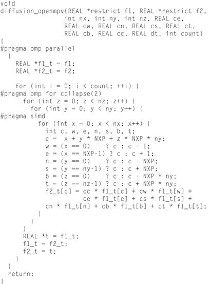
Figure 4.7 The diffusion_openmpv Function.
The line #pragma simd requests the compiler to vectorize the loop regardless of potential dependencies or other potential constraints.
That was a pretty simple one line change but we created a new file for it called diffusion_ompvect.c. Compile it with the following:
$ icc –openmp –mmic –std=c99 –O3 –vect-report=3 diffusion_ompvect.c -0 diffusion_ompvect
Note that you now should see that the vector report indicates the inner loop was indeed vectorized.
Upload the file to the coprocessor and perform four runs from the coprocessor prompt adjusting the threads per core based on the number of cores for the coprocessor on each run as below:
% export KMP_AFFINITY=scatter
% export OMP_NUM_THREADS=244
% ./diffusion_ompvect
Running diffusion kernel 6553 times
Elapsed time : 18.664 (s)
FLOPS : 76575.266 (MFlops)
Throughput : 70.685 (GB/s)
Accuracy : 1.558128e-05
% export OMP_NUM_THREADS=183
% ./diffusion_ompvect
Running diffusion kernel 6553 times
Elapsed time : 19.569 (s)
FLOPS : 73034.367 (MFlops)
Throughput : 67.416 (GB/s)
Accuracy : 1.558128e-05
% export OMP_NUM_THREADS=122
% ./diffusion_ompvect
Running diffusion kernel 6553 times
Elapsed time : 25.369 (s)
FLOPS : 56337.496 (MFlops)
Throughput : 52.004 (GB/s)
Accuracy : 1.558128e-05
% export OMP_NUM_THREADS=61
% ./diffusion_ompvect
Running diffusion kernel 6553 times
Elapsed time : 30.993 (s)
FLOPS : 46114.676 (MFlops)
Throughput : 42.567 (GB/s)
Accuracy : 1.558128e-05
Figure 4.8 shows a graph of the benefits we have seen so far. We see the significant impact of vectorization. Improving top performance by more than 4.5 times above our OpenMP changes alone and now more than 335 times our original single-threaded baseline!
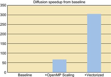
Figure 4.8 Accumulative Performance Benefits of Scaling and Vectorization.
So, we have found our Thunder Road enabling us to arrive sooner at our proverbial grocery store. We now have both scaled and vectorized our code, and we have seen very significant performance improvement over the baseline. Now we’ll look to do a little more tuning of our “engine” to see if we can gain a bit more performance.
Peeling out: peeling code from the inner loop
Okay, we could not help ourselves from stretching our sports car analogy to the limit and adding in a little pun for good measure. Peeling out or pushing hard on the gas pedal to get a car moving fast from a standstill with a little bit of tire screeching may get you to your destination a little bit faster but probably not with the large improvements we have found so far. Given the dramatic speedups we have achieved with scaling and vectorizing the code, we now are looking towards finer-grained tuning.

In this section, we will look to remove or “peel” unneeded code from the inner loop. Reviewing the code carefully, we see that the boundary check might be a candidate. Consider that for a volume of any significant size, the code will encounter a boundary that requires altering the baseline stencil usage relatively rarely. If possible, we want to look for a way to “peel out” the boundary checks from the inner loop portions because we know that the code does the bulk of its processing without encountering a boundary condition. Figure 4.9 shows one way to do it.
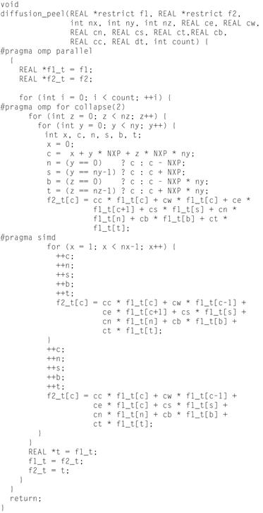
Figure 4.9 The diffusion_peel Function.
Since only our starting and ending x coordinates 0 and nx−1 will hit the boundary condition, we can create an inner loop without any boundary checks by simply ensuring we process x indices from 1 to nx−2. Furthermore, since the stencil always traverses in single units across the x row of sub-volumes, we can update the stencil positions by simply incrementing them. Also, we can eliminate calculating the east and west locations by referencing their positions directly in the array index (e=c−1 and w=c+1). This new inner loop now has the X-edge checks removed. The file diffusion_peel.c contains the code with the modifications. We can compile and run it to see if we achieved any improvement as below
$ icc –openmp –mmic –std=c99 –O3 –vect-report=3 diffusion_peel.c -0 diffusion_peel
Upload the file to your working directory on the coprocessor. Set the affinity and number of threads at the coprocessor prompt iterating through the number of threads needed (based on core count) to perform one to four threads per core using the following commands:
% export KMP_AFFINITY=scatter
% export OMP_NUM__THREADS=244
% ./diffusion_peel
Running diffusion kernel 6553 times
Elapsed time : 15.111 (s)
FLOPS : 94585.055 (MFlops)
Throughput : 87.309 (GB/s)
Accuracy : 1.580171e-05
% Export OMP_NUM_THREADS=183
% ./diffusion_peel
Running diffusion kernel 6553 times
Elapsed time : 18.980 (s)
FLOPS : 75303.023 (MFlops)
Throughput : 69.510 (GB/s)
Accuracy : 1.580171e-05
% export OMP_NUM_THREADS=122
% ./diffusion_peel
Running diffusion kernel 6553 times
Elapsed time : 18.217 (s)
FLOPS : 78457.055 (MFlops)
Throughput : 72.422 (GB/s)
% export OMP_NUM_THREADS=61
% ./diffusion_peel
Running diffusion kernel 6553 times
Elapsed time : 23.815 (s)
FLOPS : 60013.832 (MFlops)
Throughput : 55.397 (GB/s)
Accuracy : 1.580171e-05
As expected, we got a measureable improvement in our fastest run (244 threads) but it certainly is not as dramatic as we have seen before. However, we did improve by almost 24 percent over our prior code runs, which is a solid and beneficial improvement.
In the next sections, we will look at one more possible improvement that should be part of our standard fine-tuning repertoire.
Trying higher octane fuel: improving speed using data locality and tiling
Many high-performance cars benefit from using fuel with a higher octane rating. So far we have optimized the direction and roads we are traveling on and added some touches to get moving faster. Now we will attempt one final improvement by trying to get more power out of our fuel, the memory subsystem.
In many circumstances, improvements can be found by analyzing the data access patterns to take advantage of data locality. We want to create a more optimal pattern of data reuse within our innermost loops to maintain data in the L1 and L2 caches for much faster access.
Stencil operations contain data reuse patterns that make them strong candidates for exploiting data locality. Tiling and blocking are terms to describe a technique often used for improving data reuse in cache architectures. Cache architectures generally employ “least recently used” (LRU) methods to determine which data is evicted from the cache as new data is requested. Therefore, the longer data remains unused, the more likely it will be evicted from the cache and no longer available immediately when needed. Since memory accesses are significantly longer than cache accesses, a goal is to find techniques and usage patterns that can help reduce memory accesses by reusing cached data. To be most successful, reusing data in cache lines that have been used very recently or local to current code sequence is important.
Tiling the access pattern can exploit data that remains in the cache from recent, previous iterations. For instance, in our diffusion stencil code, each innermost loop iteration processes the x elements of a y row sequentially, and then moves on to the following y row. Ignoring the work division from scheduling multiple threads for a moment, there is a high likelihood of accessing data in the L1 or L2 cache we have used before from the current and previous y rows since our access of those y data is recent. However, the bottom and top row data on the adjacent z plane are used once and then not accessed again until the next full y plane is processed at the same row. Therefore, there is a low likelihood that the z data are being reused and so they must be fetched again from memory on the next iteration of the z loop. If we consider processing a rectangular tile of y—actually a slab of yx values across a range of z. The top row in a given z iteration will still be in cache to serve as left, center, and right rows for the next z, and the bottom row for the z after that. This usage avoids additional memory requests and a performance benefit is likely possible. Figure 4.10 depicts an example of the cache access and reuse level we should be able to achieve if we tile in y and step across the z dimension within those tiles. Each block represents a 64-byte cache line, which holds sixteen contiguous x-dimension single-precision float values. The saturated highlights the reuse pattern with darker blocks representing multiple reuse of the same value across a range of y and z.
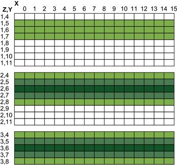
Figure 4.10 Cache Line Reuse in Diffusion Calculation.
Figure 4.11 shows a code implementation of the diffusion_tiled() function. We select a blocking factor value YBF for the number of y rows we will process in each slab; the goal being to select an optimal number that will maintain the sufficient amounts of y and z data in the cache long enough to be reused during computation.


Figure 4.11 The diffusion_tiled Function.
Since we will be processing a portion or tile of y rows across the full z dimension, we add an outer y loop to control stepping to the start of each tile. The inner y loop is then adjusted to perform the per-row processing within the current tile. The x processing with the peeled out boundary management is maintained so we keep that optimization intact.
So, let’s compile, upload, and run the code on our coprocessor.
$ icc –openmp –mmic –std=c99 –O3 –vect-report=3 diffusion_tiled.c -0 diffusion_tiled
Upload the code and go to the coprocessor command prompt and run the program with each of the threads per core available:
% export KMP_AFFINITY=scatter
% export OMP_NUM_THREADS=244
% ./diffusion_tiled
Running diffusion kernel 6553 times
Elapsed time : 16.151 (s)
FLOPS : 88490.656 (MFlops)
Throughput : 81.684 (GB/s)
Accuracy : 1.580171e-05
% export OMP_NUM_THREADS=183
% ./diffusion_tiled
Running diffusion kernel 6553 times
Elapsed time : 13.388 (s)
FLOPS : 106752.742 (MFlops)
Throughput : 98.541 (GB/s)
Accuracy : 1.580171e-05
% export OMP_NUM_THREADS=122
Running diffusion kernel 6553 times
Elapsed time : 16.704 (s)
FLOPS : 85561.117 (MFlops)
Throughput : 78.979 (GB/s)
% export OMP_NUM_THREADS=61
Running diffusion kernel 6553 times
Elapsed time : 30.993 (s)
FLOPS : 46114.676 (MFlops)
Throughput : 42.567 (GB/s)
Accuracy : 1.558128e-05
The improved cache reuse gave us a bit more of a boost and we ended up with another 15-percent improvement over the peel improvements. That is 435 times improvement from the original single-threaded baseline. Figure 4.12 shows a graph of the performance improvements we realized while tuning the diffusion code. As with any code, there are likely some other improvements we could find with deeper analysis, particularly targeted ones with the help of analysis tools like Intel VTune Amplifier. But for our goals of this book on essentials, you have seen some of the key steps and “parallel thinking” needed to take real-world code from a serial implementation to high-speed parallel code that remains general and portable while scaling across cores and threads, and taking advantage of vectorization and cache architecture.

Figure 4.12 Accumulative Performance Improvements from Baseline to Tiling.
High speed driver certificate: summary of our high speed tour

Congratulations! You now have completed our introductory high speed “driving course” for parallel, high performance programming using the Intel Xeon Phi coprocessor. In these last three chapters, our goal was to give you an immediate hands-on, practical feel for tapping the performance potential of this new and exciting Intel product. However, it is important to understand that the parallel programming techniques, development tools, and methods we used are universally applicable to most any general purpose, parallel computing platform. For instance, the code also should see measurable performance improvements through each optimization step on past, present, and future Intel® Xeon® processors with multiple cores.
Ultimately, you can look at the Intel Xeon Phi coprocessor with its Intel Many Integrated Core architecture as taking computing architecture for parallel processing to a new level. As a software developer, to enjoy any real benefit on an Intel Xeon Phi coprocessor you must focus on parallel coding techniques or you will likely end up quite disappointed with the results on the coprocessor. We have found that, when the investment is made in optimizing code for parallel techniques such as vectorizing and scaling for multiple cores while reducing cross-task or thread dependencies, code can perform hundreds or even thousands of times faster than the original serial version. Furthermore, your investment in parallelism pays dividends; providing improvements with many currently available processors while poised to gain further benefits as parallel computing continues to be the foreseeable norm.
We now will switch gears from practice to theory in the upcoming chapters. We will give you more insight how to exploit more parallelism in your applications and take full advantage of the Intel Xeon Phi coprocessor.