
Chapter 3
Three-point non-optimal methods
In Chapter 2 we have presented several two-point methods with order of convergence three and four. None of these methods has order higher than four, which supports the Kung-Traub conjecture that the upper bound of the order of convergence of ![]() -point methods requiring
-point methods requiring ![]() function evaluations is
function evaluations is ![]() . In this chapter we will study three-point methods whose order also cannot reach the Kung-Traub bound
. In this chapter we will study three-point methods whose order also cannot reach the Kung-Traub bound ![]() . Recall that the abbreviation
. Recall that the abbreviation ![]() denotes the number of function evaluations. We study non-optimal three-point methods because their design is based on a variety of different, inspiring, and genuine developing techniques that finally led, step by step, to the methods of optimal order. It turned out that these techniques, including various types of interpolations, approximations using Taylor’s series, and weight functions, are particularly useful for constructing higher order optimal multipoint methods, discussed in later chapters.
denotes the number of function evaluations. We study non-optimal three-point methods because their design is based on a variety of different, inspiring, and genuine developing techniques that finally led, step by step, to the methods of optimal order. It turned out that these techniques, including various types of interpolations, approximations using Taylor’s series, and weight functions, are particularly useful for constructing higher order optimal multipoint methods, discussed in later chapters.
3.1 Some historical notes
We have seen in Chapter 2 that Ostrowski (1960), Jarratt (1966, 1969), and King (1973a) created first optimal two-point methods of order 4. The next optimal methods, constructed and published by Kung and Traub (1974) and discussed in Section 5.2, are not only optimal but also possess arbitrary order![]() for any integer
for any integer ![]() . In the period 1974–2007, except Neta’s four-point method (Neta, 1983) with optimal order 16, none of developed three-point methods reached optimal order 8 (see Remark 5.3).
. In the period 1974–2007, except Neta’s four-point method (Neta, 1983) with optimal order 16, none of developed three-point methods reached optimal order 8 (see Remark 5.3).
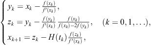
The three-point methods of order 8, obtained from the Kung-Traub families (2.109) and (2.110), or generated by a program given in Section 5.2, can be represented by the following two iterative formulas:
Derivative free K-T family (Kung and Traub, 1974):
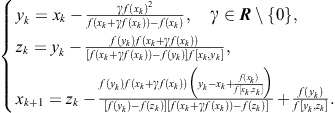 (3.1)
(3.1)
K-T family with first derivative (Kung and Traub, 1974):
 (3.2)
(3.2)
A convergence theorem for the Kung-Traub general ![]() -point methods will be considered in Section 5.2.
-point methods will be considered in Section 5.2.
In the decade after Kung-Traub’s families (2.109) and (2.110), several ![]() -point methods
-point methods ![]() appeared in the papers of Neta (1979, 1981, 1983), Popovski (1981), and King (1973a, 1973b). Some of the methods presented therein were constructed in different ways or they use more than one initial approximation, which complicates their proper comparison to optimal multipoint methods. We will return to these methods later.
appeared in the papers of Neta (1979, 1981, 1983), Popovski (1981), and King (1973a, 1973b). Some of the methods presented therein were constructed in different ways or they use more than one initial approximation, which complicates their proper comparison to optimal multipoint methods. We will return to these methods later.
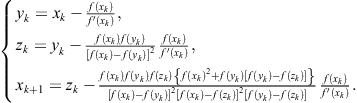
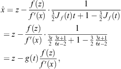
Taking King’s method (2.57) for arbitrary ![]() at the first two steps and the same method in the third step for
at the first two steps and the same method in the third step for ![]() , Neta (1979) derived the following sixth-order method:
, Neta (1979) derived the following sixth-order method:
 (3.3)
(3.3)
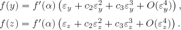
The asymptotic error constant of this method is
![]()
To our knowledge, this was the first three-point method of sixth order with ![]() .
.
The next three-point methods with optimal order 8, in an explicit way, appeared many years after Kung-Traub’s families in Milovanović and Cvetković (2007) and the articles (Bi et al., 2009a,b) of Bi, Ren, and Wu. However, it is worth noting that a much faster four-point method of optimal order 16 was constructed in 1983 in Neta’s paper (Neta, 1983). This method relies on a three-point method of eighth order, given implicitly. This fact opens a question of the priority between Neta’s work and mentioned results from 2007 to 2009, see Remark 5.3. In the meantime, between 1974 and 2007, many three-point methods with order less than 8 were developed. After the quoted works of Bi et al., a dozen of eighth-order three-point methods were constructed using various techniques and ideas.
3.2 Methods for constructing sixth-order root-finders
Before considering optimal three-point methods (Chapter 4), we demonstrate various techniques for developing three-point methods; we start from an arbitrary two-point method of optimal order 4 and always construct methods of sixth order. For simplicity, we omit the iteration index and denote a new approximation by ![]() . Besides, if
. Besides, if ![]() are approximations to the zero
are approximations to the zero ![]() of
of ![]() , we introduce the associated errors
, we introduce the associated errors
![]()
Let ![]() be the class of optimal two-point methods of order 4, which require three function evaluations, and let
be the class of optimal two-point methods of order 4, which require three function evaluations, and let ![]() be an I.F. consisting of two steps. We distinguish between two cases:
be an I.F. consisting of two steps. We distinguish between two cases:
(I) The first step relies on a Newton-like method of quadratic convergence, say
![]()
Without loss of generality, we can choose the Newton method because other quadratically convergent methods reduce to Newton’s method (a member of Schröder’s sequence) according to Theorem 1.7. An iteration function ![]() is then constructed using
is then constructed using ![]() , and
, and ![]() .
.
(II) The first step is the Steffensen-like method of quadratic convergence
![]() (3.4)
(3.4)
An iteration function ![]() is constructed using
is constructed using ![]() , and
, and ![]() .
.
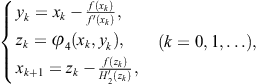
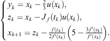
We will construct three-point methods starting from the following three-step scheme:
 (3.5)
(3.5)
with the idea to approximate ![]() using available data
using available data ![]() or
or ![]() (four F.E. in total per iteration).
(four F.E. in total per iteration).
We note that
 (3.6)
(3.6)
where ![]() is the asymptotic error constant of the method defined by
is the asymptotic error constant of the method defined by ![]() . Observe that the order of convergence of the iterative scheme (3.5) is 8 (according to Theorem 1.3), but its computational efficiency is low since five F.E. are required.
. Observe that the order of convergence of the iterative scheme (3.5) is 8 (according to Theorem 1.3), but its computational efficiency is low since five F.E. are required.
In what follows, we use Taylor’s expansions
 (3.7)
(3.7)
and
 (3.8)
(3.8)
3.2.1 Method 1 – Secant-like method
Using (3.6) and (3.8), we find
![]()
Hence, we approximate ![]() and, by substituting into (3.5), we obtain
and, by substituting into (3.5), we obtain

Therefore, according to the last relation, it follows that the three-point secant-like method:
 (3.9)
(3.9)
is of sixth order for arbitrary optimal two-step method used in the first two steps. The increase of order from 4 to 6 is attained with one additional function evaluation.
3.2.2 Method 2 – Rational bilinear interpolation
To approximate the derivative ![]() in (3.5), we use the interpolation by a rational function
in (3.5), we use the interpolation by a rational function
![]() (3.10)
(3.10)
The unknown coefficients ![]() , and
, and ![]() are determined from the conditions
are determined from the conditions ![]() . It is easy to find
. It is easy to find
![]()
Now we substitute

and state a three-point method
 (3.11)
Substituting (3.6)–(3.8) into the expression of ![]() , after the expansion of
, after the expansion of ![]() in Taylor’s series in terms of the error
in Taylor’s series in terms of the error ![]() and lengthy calculation, we obtain
and lengthy calculation, we obtain
![]()
which means that the three-point method (3.11) is of order 6.
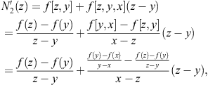
3.2.3 Method 3 – Hermite’s interpolation
The derivative ![]() in (3.5) can also be approximated using Hermite’s interpolating polynomial of second degree
in (3.5) can also be approximated using Hermite’s interpolating polynomial of second degree
![]() (3.12)
(3.12)
from the available data ![]() . We will show that the iterative method arising from the three-step scheme (3.5) is of order 6. We show in Section 4.2 that the use of Hermite’s interpolating polynomial of third degree with additional information
. We will show that the iterative method arising from the three-step scheme (3.5) is of order 6. We show in Section 4.2 that the use of Hermite’s interpolating polynomial of third degree with additional information ![]() can provide three-point methods of optimal order 8.
can provide three-point methods of optimal order 8.
The unknown coefficients ![]() , and
, and ![]() in (3.12) are determined by the conditions
in (3.12) are determined by the conditions
![]()
It is easy to find
![]()
Hence
![]() (3.13)
(3.13)
In convergence analysis of multipoint methods considered in this book, we use the following well-known expression for the error of the Hermite interpolation (see, e.g., Traub, 1964, p. 244).
Theorem 3.1
Let ![]() and its derivatives
and its derivatives ![]() be continuous in the smallest interval
be continuous in the smallest interval ![]() that contains all interpolation nodes
that contains all interpolation nodes ![]() . Let
. Let ![]() be Hermite’s interpolating polynomial of degree
be Hermite’s interpolating polynomial of degree ![]() constructed using the nodes
constructed using the nodes ![]() with respective multiplicities
with respective multiplicities ![]() such that
such that
![]()
Then
![]() (3.14)
(3.14)
where ![]() .
.
Let us consider the special case of (3.14) when ![]() , and
, and ![]() are the multiplicities of the nodes
are the multiplicities of the nodes ![]() and
and ![]() , respectively. Then
, respectively. Then
![]()
and hence, for ![]() ,
,
![]() (3.15)
(3.15)
According to (3.6) we have ![]() and from (3.15) there follows:
and from (3.15) there follows:
![]()
Regarding the third step of (3.5), we find
![]() (3.16)
(3.16)
In view of (3.8),
![]()
Returning to (3.16) we obtain
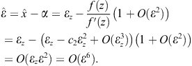
Therefore, the three-point method
 (3.17)
obtained by the Hermite interpolating polynomial of second degree, has sixth order of convergence.
3.2.4 Method 4 – Inverse interpolation
To get a three-point sixth-order method using four function evaluations, we use the inverse interpolation by the quadratic polynomial
![]() (3.18)
(3.18)
Substituting ![]() yields
yields
![]()
Differentiating (3.18) we get
![]()
Hence, for ![]() ,
,
![]()
Using the values of the coefficients ![]() and
and ![]() , from (3.18) we find
, from (3.18) we find
![]()
Assume that ![]() is a zero of
is a zero of ![]() , that is,
, that is, ![]() . Then we have from (3.18)
. Then we have from (3.18)
![]() (3.19)
(3.19)
According to this, the following three-step method is obtained:
![]() (3.20)
(3.20)
for ![]() Note that the first and second step are implicitly defined as
Note that the first and second step are implicitly defined as ![]() and
and ![]() . In this case the third step in (3.20) has a specific form different from Newton’s step in (3.5).
. In this case the third step in (3.20) has a specific form different from Newton’s step in (3.5).
Replacing the relation (3.6) and the expansions (3.7) and (3.8) in (3.19), we arrive at the error relation
![]()
This proves that the order of convergence of the three-point method (3.20) is 6. Recall that ![]() is the asymptotic error constant of (arbitrary chosen) optimal fourth-order method
is the asymptotic error constant of (arbitrary chosen) optimal fourth-order method ![]() .
.
3.2.5 Method 5 – Newton’s interpolation
Assume that a given function ![]() is represented by a set of values
is represented by a set of values ![]() at distinct points (nodes)
at distinct points (nodes) ![]() . For this set of data it is possible to construct Newton’s interpolating polynomial of degree
. For this set of data it is possible to construct Newton’s interpolating polynomial of degree ![]() with divided differences
with divided differences
![]() (3.21)
(3.21)
satisfying interpolation conditions ![]() . Recall that the divided difference of the
. Recall that the divided difference of the ![]() th order is defined recursively by (2.3).
th order is defined recursively by (2.3).
To construct three-point methods, we apply Newton’s interpolating polynomial (3.21) for ![]() taking three different choices of nodes:
taking three different choices of nodes:
First we consider the choice (a) taking the Steffensen-like method (3.4) in the first step of scheme (1)–(3). Newton’s interpolating polynomial takes the form
![]() (3.22)
(3.22)
Proceeding as before, we replace ![]() in (3.5) by
in (3.5) by ![]() . Differentiating (3.22) we obtain for
. Differentiating (3.22) we obtain for ![]()

whence
![]() (3.23)
(3.23)
Since ![]() ,
, ![]() , we get by Taylor’s series
, we get by Taylor’s series
 (3.24)
Substituting (3.6)–(3.8) and (3.24) into (3.23) and using Taylor’s series, we find
![]() (3.25)
(3.25)
By virtue of (3.6), (3.8), and (3.25), from (3.5) we find
 (3.26)
As above, ![]() is the asymptotic error constant of the two-point method
is the asymptotic error constant of the two-point method ![]() that appears in the iterative scheme (3.5).
that appears in the iterative scheme (3.5).
Now we consider the choice (b). Newton’s interpolating polynomial has the form
![]() (3.27)
(3.27)
We want to replace ![]() in (3.5) by
in (3.5) by ![]() . Differentiating (3.27) we obtain for
. Differentiating (3.27) we obtain for ![]()
giving
![]() (3.28)
(3.28)
Since we use Steffensen-like method (3.4), then ![]() , see (3.6). Substitute this error,
, see (3.6). Substitute this error, ![]() and the expansions (3.7) and (3.8) in (3.28). Using again Taylor’s series, we find
and the expansions (3.7) and (3.8) in (3.28). Using again Taylor’s series, we find
 (3.29)
Taking into account (3.6), (3.8), and (3.29), from (3.5) we find
 (3.30)
Convergence analysis for the choice (c) with Newton’s method in the first step of the scheme (3.5) is very similar to that as Steffensen-like method is applied (with ![]() instead of
instead of ![]() ). In this case we use the errors
). In this case we use the errors ![]() ,
, ![]() and the expansions (3.7) and (3.8) in (3.28). Applying Taylor’s series again, we obtain
and the expansions (3.7) and (3.8) in (3.28). Applying Taylor’s series again, we obtain
![]() (3.31)
(3.31)
Using (3.6), (3.8), and (3.31), from (3.5) we find
 (3.32)
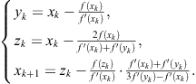
The corresponding three-point methods, constructed by Newton’s interpolation with divided differences, are given below:


According to (3.26) we conclude that the three-point derivative free methods (3.33) have order 6 (choice (a)). In regard to the error relations (3.30) and (3.32) it follows that the order of convergence of the three-point methods (3.34) and (3.35) is 7. It is clear that the methods (3.34) and (3.35) are faster than (3.33) since the approximations ![]() , and
, and ![]() , taken as nodes in (3.34) and (3.35), are better than
, taken as nodes in (3.34) and (3.35), are better than ![]() , and
, and ![]() used in (3.33).
used in (3.33).
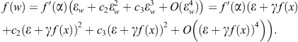
3.2.6 Method 6 – Taylor’s approximation of derivative
Many multipoint methods derived in the first decade of 21st century were derived using different approximations of the first derivative that appears at the second or third step. We will now present a simple method for approximating the derivative ![]() at the third step (3.5) of the iterative scheme (1)–(3).
at the third step (3.5) of the iterative scheme (1)–(3).
Let ![]() be a real-valued function of the argument
be a real-valued function of the argument ![]() , where
, where ![]() is the Newton approximation. Assume that
is the Newton approximation. Assume that ![]() is at least twice differentiable on an interval
is at least twice differentiable on an interval ![]() that contains a zero
that contains a zero ![]() of
of ![]() . According to (3.6)–(3.8) we find
. According to (3.6)–(3.8) we find
![]()
which means that ![]() is a very small quantity in magnitude if
is a very small quantity in magnitude if ![]() is close enough to the zero
is close enough to the zero ![]() . Hence, it is reasonable to represent
. Hence, it is reasonable to represent ![]() by its Taylor’s polynomial
by its Taylor’s polynomial ![]() in a neighborhood of the point
in a neighborhood of the point ![]() .
.
The next step is to approximate ![]() in (3.5) of the scheme (1)–(3) as follows:
in (3.5) of the scheme (1)–(3) as follows:
![]() (3.36)
(3.36)
where we put ![]() . From (3.6) we observe that
. From (3.6) we observe that
![]()
where ![]() and
and ![]() are some constants depending on the form of
are some constants depending on the form of ![]() . According to this relation and the expansions (3.7) and (3.8) for
. According to this relation and the expansions (3.7) and (3.8) for ![]() and
and ![]() , we start from
, we start from
![]()
and estimate
 (3.37)
The method given by the three-step scheme (1)–(3) with the approximation (3.36) will reach the order 6 if we choose ![]() , and
, and ![]() in (3.37) so that the coefficients next to
in (3.37) so that the coefficients next to ![]() and
and ![]() vanish. It is easy to see from (3.37) that we have to take
vanish. It is easy to see from (3.37) that we have to take
![]() (3.38)
(3.38)
Such a choice leads to the error relation
![]() (3.39)
(3.39)
where ![]() is the asymptotic error constant of the two-point method defined by
is the asymptotic error constant of the two-point method defined by ![]() .
.
According to the previous consideration, the following sixth-order method can be constructed:
 (3.40)
where the weight function ![]() satisfies the condition (3.38). We list some simple weight functions
satisfies the condition (3.38). We list some simple weight functions ![]() satisfying (3.38):
satisfying (3.38):

3.3 Ostrowski-like methods of sixth order
Using the Ostrowski two-point method (2.47) Chun and Ham (2007b) have developed a family of three-point methods using a parametric function in the third step. They have started from the three-step scheme
 (3.41)
where ![]() and
and ![]() is a real-valued function. This function has to be selected so that the order of convergence of the family (3.41) becomes as high as possible. The following theorem was proved in Chun and Ham (2007b).
is a real-valued function. This function has to be selected so that the order of convergence of the family (3.41) becomes as high as possible. The following theorem was proved in Chun and Ham (2007b).
Theorem 3.2
Let ![]() be a simple zero of at least twice differentiable function
be a simple zero of at least twice differentiable function ![]() in an open interval
in an open interval ![]() and
and ![]() any function satisfying
any function satisfying ![]() and
and ![]() . If
. If ![]() is a sufficiently good initial approximation to
is a sufficiently good initial approximation to ![]() , then the family of three-point methods (3.41)is of sixth order, and satisfies the error relation
, then the family of three-point methods (3.41)is of sixth order, and satisfies the error relation
![]() (3.42)
(3.42)
As in the case of most iterative methods, the proof is derived by using Taylor’s series. Symbolic computation in a computer algebra system (say, Mathematica or Maple) is recommended. The efficiency index of the methods (3.41) is ![]() , which is less than the efficiency index of optimal two-point methods
, which is less than the efficiency index of optimal two-point methods ![]() .
.
Taking different forms of the weight function ![]() that satisfy the conditions of Theorem 3.2, it is possible to obtain a variety of Ostrowski-like three-point methods defined by (3.41). The following examples are presented in Chun and Ham (2007b):
that satisfy the conditions of Theorem 3.2, it is possible to obtain a variety of Ostrowski-like three-point methods defined by (3.41). The following examples are presented in Chun and Ham (2007b):
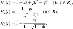
Let us observe that ![]() is of King’s type, see the King two-point method (2.57). Note that the choice
is of King’s type, see the King two-point method (2.57). Note that the choice ![]() gives the simplest form of
gives the simplest form of ![]() .
.
Remark 3.1
Chun-Ham’s method (3.41) gives some interesting particular cases which contain previously developed methods. Taking
![]()
in (3.41), one obtains the Ostrowski-King-like method considered by Sharma and Guha (2007). A sub-special case developed a year ago by Grau and Diaz-Barrero (2000) follows for ![]() , which could be named the double Ostrowski-like method.
, which could be named the double Ostrowski-like method.
Remark 3.2
Chun and Ham have chosen Ostrowski’s method (2.47) at the first two steps. However, analysis given above for the three-point methods (3.40) shows that any two-point method of optimal order 4 can be taken instead of Ostrowski’s method. This means that the family (3.41) is a special case of the family (3.40). Since the asymptotic error constant of Ostrowski’s method is
![]()
substituting this expression in (3.39) we obtain the error relation (3.42).
Remark 3.3
As mentioned above, the family (3.40) allows any two-point method of optimal order 4 at the first two steps. Neta’s method (3.3) presented at the beginning of this chapter is a special case of the family (3.40) taking King’s method (2.57) for arbitrary ![]() at the first two steps and the function
at the first two steps and the function ![]() in the third step. It is easy to check that this function satisfies
in the third step. It is easy to check that this function satisfies
![]()
3.4 Jarratt-like methods of sixth order
In Section 2.6 we have presented several two-point methods of Jarratt’s type for solving nonlinear equations. Among these Jarratt-like methods, the most frequently used and cited is the simplest method (2.146) of the form
 (3.43)
where
![]()
and the error relation
![]() (3.44)
(3.44)
holds.
To accelerate Jarratt’s method (3.43), Kou and Li (2007) have used the linear interpolation at two points ![]() and
and ![]() , that is,
, that is,
![]()
and approximated
 (3.45)
Combining (3.43), (3.45), and the third step
![]() (3.46)
(3.46)
the following three-step method of Jarratt’s type was derived in (Kou and Li, 2007)
 (3.47)
The corresponding error relation is given by
![]() (3.48)
(3.48)
which means that the order of convergence of the three-point method (3.47) is 6 (see Kou and Li (2007) for the complete proof). The efficiency index is ![]() .
.
Using a similar approach and the approximation of ![]() by the parabola
by the parabola ![]() through the points
through the points ![]() and
and ![]() , Chun (2007d) obtained the approximation
, Chun (2007d) obtained the approximation

Replacing this approximation into (3.46), a slight generalization of the sixth-order method (3.47) was stated in (Chun, 2007d),
 (3.49)
Evidently, if ![]() then (3.49) reduces to (3.47).
then (3.49) reduces to (3.47).
Now we will consider two Jarratt-like families of sixth order based on the family (2.147). We start from the three-step scheme
 (3.50)
where ![]() and
and ![]() is a real-valued function that satisfies the following conditions:
is a real-valued function that satisfies the following conditions:
![]() (3.51)
(3.51)
To decrease the number of F.E. in (3.50), ![]() is approximated using Hermite’s interpolation, see Method 3 in Section 3.2. We use the nodes
is approximated using Hermite’s interpolation, see Method 3 in Section 3.2. We use the nodes ![]() (of multiplicity 2) and
(of multiplicity 2) and ![]() (of multiplicity 1) to construct Hermite’s interpolating polynomial
(of multiplicity 1) to construct Hermite’s interpolating polynomial
![]()
where we omit the iteration index for simplicity.
The unknown coefficients ![]() , and
, and ![]() are determined from the conditions
are determined from the conditions
![]()
whence
![]()
For ![]() we obtain
we obtain
![]()
that is, the expression (3.13). Now, we substitute ![]() and, proceeding as in Section 3.2 (see (3.13)–(3.16)), we prove that the family of three-point methods
and, proceeding as in Section 3.2 (see (3.13)–(3.16)), we prove that the family of three-point methods
 (3.52)
is of order 6.
The second approach applies the aforementioned Method 6 (Taylor’s approximation of derivative) in the third step of (3.50) to approximate ![]() . We proceed as follows:
. We proceed as follows:
![]() (3.53)
(3.53)
![]()
is Taylor’s polynomial of second degree.
First we find by Taylor’s series
 (3.54)
and
![]() (3.55)
(3.55)
where
![]()
is the coefficient of ![]() in (2.149). By virtue of (3.54) and (3.55) we find
in (2.149). By virtue of (3.54) and (3.55) we find
 (3.56)
The three-point method (3.50) with the approximation (3.53) will reach order 6 if the coefficients of ![]() and
and ![]() in (3.56) vanish. It is easy to show that this requirement will be satisfied if we take
in (3.56) vanish. It is easy to show that this requirement will be satisfied if we take
![]() (3.57)
(3.57)
Putting these values in (3.56) we arrive at the error relation
![]() (3.58)
(3.58)
According to (3.58) we conclude that the family of three-point methods
 (3.59)
is of order 6 if the function ![]() satisfies the conditions (3.57) and
satisfies the conditions (3.57) and ![]() satisfies (3.51).
satisfies (3.51).
The third approach relies on the general form of two-point family of Jarratt’s type presented in the scheme (3.50) and the linear interpolation at the two points ![]() and
and ![]() ,
,
![]()
see (3.45). For ![]() we obtain the approximation
we obtain the approximation
![]() (3.60)
(3.60)
To find ![]() , we use Taylor’s expansions
, we use Taylor’s expansions

where ![]() (from (2.116)). With these values we find from (3.60)
(from (2.116)). With these values we find from (3.60)
![]()
The use of Taylor’s series gives
![]()
so that the error relation of (3.59) is given by
 (3.61)
Therefore the family of three-point methods of Jarratt’s type
 (3.62)
is of order 6.
Remark 3.4
In the particular case (3.43) considered by Kou and Li (2007), where ![]() , the asymptotic error constant is
, the asymptotic error constant is ![]() , see (3.44). Putting this value in (3.61) we obtain the error relation (3.48) of the method (3.47).
, see (3.44). Putting this value in (3.61) we obtain the error relation (3.48) of the method (3.47).
From (3.45) and the fact that the linear interpolation is used, it is obvious that the choice ![]() in (3.62) gives the particular method (3.47). The following question is of interest: Does the family (3.59) include the method (3.47)? First, we note that
in (3.62) gives the particular method (3.47). The following question is of interest: Does the family (3.59) include the method (3.47)? First, we note that ![]() . The third step of (3.59) can be written in the form
. The third step of (3.59) can be written in the form
where ![]() . According to (3.57), we should show that the function
. According to (3.57), we should show that the function ![]() satisfies the conditions
satisfies the conditions
![]() (3.63)
(3.63)
Taylor’s expansion of ![]() at the point
at the point ![]() gives
gives
![]() (3.64)
(3.64)
and we see that the function ![]() fulfills (3.63). This means that the method (3.47) is a member of the family (3.59). Besides, in regard to (3.64) we note that the third step of (3.47) can be written in a simpler form taking the term
fulfills (3.63). This means that the method (3.47) is a member of the family (3.59). Besides, in regard to (3.64) we note that the third step of (3.47) can be written in a simpler form taking the term
![]()
instead of ![]() , which leads to the following variant of Jarratt-like method of sixth order:
, which leads to the following variant of Jarratt-like method of sixth order:
 (3.65)
3.5 Other non-optimal three-point methods
Previous presentation includes several non-optimal three-point methods which use four F.E. but do not reach optimal order 8. A lot of non-optimal three-point methods with ![]() have appeared up to now. In this section we expand this review with a few non-optimal methods which present fruitful ideas or possess interesting structure of iterative formulae.
have appeared up to now. In this section we expand this review with a few non-optimal methods which present fruitful ideas or possess interesting structure of iterative formulae.
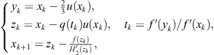
Chun and Neta (2008) have applied a method of undetermined coefficients to the three-point scheme
 (3.66)
where ![]() defines any third-order method that requires the values
defines any third-order method that requires the values ![]() . For example, Traub’s methods (2.12), (2.14), or (2.16) can be taken for
. For example, Traub’s methods (2.12), (2.14), or (2.16) can be taken for ![]() .
.
Since ![]() in (3.66), the following approximation:
in (3.66), the following approximation:
![]() (3.67)
(3.67)
was considered by Chun and Neta (2008) to decrease the computational cost. The coefficients ![]() , and
, and ![]() are calculated by the method of undetermined coefficients. Note that the use of (already calculated)
are calculated by the method of undetermined coefficients. Note that the use of (already calculated) ![]() instead of
instead of ![]() in (3.66) gives a method of order 5.
in (3.66) gives a method of order 5.
Expand the terms ![]() , and
, and ![]() about the point
about the point ![]() up to third derivative. Upon comparing the coefficients of the derivatives of
up to third derivative. Upon comparing the coefficients of the derivatives of ![]() at
at ![]() , the following system of equations for the unknowns
, the following system of equations for the unknowns ![]() , and
, and ![]() is formed:
is formed:
 (3.68)
where ![]() and
and ![]() . The solution of the system (3.68) is given by
. The solution of the system (3.68) is given by

Substituting ![]() with these coefficients in (3.67), Chun and Neta have stated the iterative method
with these coefficients in (3.67), Chun and Neta have stated the iterative method
![]() (3.69)
(3.69)
where ![]() . It was proved by Chun and Neta (2008) that the order of convergence of the method (3.66) with the last step replaced by (3.69) is 6.
. It was proved by Chun and Neta (2008) that the order of convergence of the method (3.66) with the last step replaced by (3.69) is 6.
A particular case of Chun-Neta’s scheme (3.66) with
![]() (3.70)
(3.70)
(the third-order method (2.14)) has served to Parhi and Gupta (2008) to construct the sixth-order method using a different approach. To eliminate ![]() in the third step of (3.66), they have applied the linear interpolation at the points
in the third step of (3.66), they have applied the linear interpolation at the points ![]() and
and ![]() ,
,
![]()
Hence, for ![]() , we again obtain (3.60).
, we again obtain (3.60).
Substituting the Newton approximation ![]() and (3.70) in (3.60), one obtains
and (3.70) in (3.60), one obtains
![]()
Taking into account this approximation, the iterative scheme (3.66) with (3.70) leads to Parhi-Gupta’s three-point method
 (3.71)
Parhi and Gupta (2008) have derived the error relation
![]()
proving that the order of convergence of the three-point method (3.71) is 6.
We end this section with two three-point methods of order 7. The first method was developed by Kou et al. (2007d). Introducing
![]()
a class of third-order methods, called Chebyshev-Halley’s methods, is given by
![]() (3.72)
(3.72)
see Amat et al. (2003) and Gutiérrez and Hernández (1997).
Let ![]() be the Newton approximation. Taylor’s expansion of
be the Newton approximation. Taylor’s expansion of ![]() about
about ![]() gives
gives
![]()
Hence ![]() so that
so that
![]() (3.73)
(3.73)
Substituting (3.73) in (3.72) yields Kou-Li-Wang’s two-point method (Kou et al., 2007d)
![]() (3.74)
(3.74)
where
![]()
The iterative method (3.74) satisfies the following error relation:
![]() (3.75)
(3.75)
Putting ![]() in (3.75) gives Traub’s method (2.25), rediscovered later by Potra and Pták (1984). The choice
in (3.75) gives Traub’s method (2.25), rediscovered later by Potra and Pták (1984). The choice ![]() produces Ostrowski’s method (2.47) with order 4.
produces Ostrowski’s method (2.47) with order 4.
The iterative method (3.74) has served as the base for constructing the following class of three-point methods (Kou et al., 2007d):
 (3.76)
The order of convergence of the iterative methods (3.76) is given in the theorem below, see Kou et al. (2007d).
Theorem 3.3
Suppose that ![]() is a simple zero of a function
is a simple zero of a function ![]() on an open interval
on an open interval ![]() . If
. If ![]() is a reasonably good initial approximation to
is a reasonably good initial approximation to ![]() and
and ![]() is sufficiently smooth in the neighborhood of
is sufficiently smooth in the neighborhood of ![]() , then the three-point methods (3.76)have order 7 for any
, then the three-point methods (3.76)have order 7 for any![]() and satisfy the following error relation:
and satisfy the following error relation:
![]()
Remark 3.5
The error relation given in Theorem 3.3 was derived using eight terms in all Taylor’s expansions and it differs from that derived by Kou et al. (2007d) where less terms of expansions were employed delivering, as a consequence, imprecise asymptotic error constant
![]()
The second three-point method was constructed by Bi et al. (2008) starting from the three-point scheme
 (3.77)
Observe that King’s method (2.57) was used in the first two steps. The order of the iterative method (3.77) is 8 but 5 F.E. are required, which gives the efficiency index ![]() . Therefore, this method is less efficient than optimal two-point methods (with
. Therefore, this method is less efficient than optimal two-point methods (with ![]() .
.
To decrease the number of function evaluations, the authors have applied a standard method in Bi et al. (2008): ![]() is approximated in the third step using available data. Using Taylor’s series at the point
is approximated in the third step using available data. Using Taylor’s series at the point ![]() , one obtains
, one obtains
![]() (3.78)
(3.78)
![]() (3.79)
(3.79)
Substituting ![]() from (3.78) in (3.79) gives
from (3.78) in (3.79) gives
 (3.80)
Assume that ![]() and
and ![]() are close enough to
are close enough to ![]() , then from (3.78) we find
, then from (3.78) we find
![]()
where the limit relation

is used. Returning to (3.80) we obtain
![]() (3.81)
(3.81)
Replacing this approximation of ![]() into (3.77), the following three-point method was stated by Bi et al. (2008):
into (3.77), the following three-point method was stated by Bi et al. (2008):
 (3.82)
The error relation of (3.82) is of the form
![]()
which shows that the family of methods (3.82) is of seventh order (see Bi et al., 2008).
References
1. Amat S, Busquier S, Gutiérrez JM. Geometric constructions of iterative functions to solve nonlinear equations. J Comput Appl Math. 2003;157:197–205.
2. Bi W, Ren H, Wu Q. New family of seventh-order methods for nonlinear equations. Appl Math Comput. 2008;203:408–412.
3. Bi W, Ren H, Wu Q. Three-step iterative methods with eight-order convergence for solving nonlinear equations. J Comput Appl Math. 2009a;225:105–112.
4. Bi W, Wu Q, Ren H. A new family of eight-order iterative methods for solving nonlinear equations. Appl Math Comput. 2009b;214:236–245.
5. Chun C. Some improvements of Jarratt’s method with sixth-order convergence. Appl Math Comput. 2007d;190:1432–1437.
6. Chun C, Ham Y. Some sixth-order variants of Ostrowski root-finding methods. Appl Math Comput. 2007b;193:389–394.
7. Chun C, Neta B. Some modification of Newton’s method by the method of undetermined coefficients. Comput Math Appl. 2008;56:2528–2538.
8. Grau M, Diaz-Barrero JL. An improvement to Ostrowski root-finding method. Appl Math Comput. 2000;173:450–456.
9. Gutiérrez JM, Hernández MA. A family of Chebyshev-Halley type methods in Banach spaces. Bull Austral Math Soc. 1997;55:113–130.
10. Jarratt P. Some fourth order multipoint methods for solving equations. Math Comp. 1966;20:434–437.
11. Jarratt P. Some efficient fourth-order multipoint methods for solving equations. BIT. 1969;9(119–124):b0060.
12. King RF. A family of fourth order methods for nonlinear equations. SIAM J Numer Anal. 1973a;10:876–879.
13. King RF. An improved Pegasus method for root finding. BIT. 1973b;13:423–427.
14. Kou J, Li Y. An improvement of the Jarratt method. Appl Math Comput. 2007;189:1816–1821.
15. Kou J, Li Y, Wang X. Some variants of Ostrowski’s method with seventh-order convergence. J Comput Appl Math. 2007d;209:153–159.
16. Kung HT, Traub JF. Optimal order of one-point and multipoint iteration. J ACM. 1974;21:643–651.
17. Milovanović GV, Cvetković AS. A note on three-step iterative methods for nonlinear equations. Stud Univ Babeş-Bolyai Math. 2007;52:137–146.
18. Neta B. A sixth order family of methods for nonlinear equations. Int J Comput Math. 1979;7:157–161.
19. Neta B. On a family of multipoint methods for nonlinear equations. Int J Comput Math. 1981;9:353–361.
20. Neta B. A new family of higher order methods for solving equations. Int J Comput Math. 1983;14:191–195.
21. Ostrowski AM. Solution of Equations and Systems of Equations. New York: Academic Press; 1960.
22. Parhi SK, Gupta DK. A sixth order method for nonlinear equations. Appl Math Comput. 2008;203:50–55.
23. Popovski DB. A note on Neta’s family of sixth order methods for solving equations. Int J Comput Math. 1981;10:91–93.
24. Potra, F.A., Pták V., 1984. Nondiscrete Induction and Iterative Processes. Research Notes in Mathematics, vol. 103, Pitman, Boston.
25. Sharma JR, Guha RK. A family of modified Ostrowski methods with accelerated sixth order convergence. Appl Math Comput. 2007;190:111–115.
26. Traub JF. Iterative Methods for the Solution of Equations. Englewood Cliffs, New Jersey: Prentice-Hall; 1964.