
16 Transact-SQL Performance Tuning
Good engineering is the difference between code running in eight minutes or eight hours. It affects real people in real ways. It’s not a “matter of opinion" any more than a bird taking flight is a “matter of opinion.”
—H. W. Kenton
General SQL Server performance tuning is outside the scope of this book. That subject alone could easily fill several volumes on its own. Instead, the focus of this chapter is on tuning the performance of Transact-SQL queries. The options are many and the tools are sometimes complex, but there are a number of specific techniques you can employ to write optimal Transact-SQL code and to improve the performance of queries that don’t perform acceptably well.
• The best thing you can do to ensure the code you write performs optimally is to deepen the level of expertise on your development team. Good developers write good code. It pays to grow development talent through aggressive training. None of us was born knowing what a correlated subquery is. Investment in people often yields long-term benefits that are difficult if not impossible to obtain otherwise.
• Identify and thoroughly investigate your application’s key database operations and transactions as early in the development process as possible. Knowing these well early on and addressing them as soon as possible can mean the difference between a successful release and a fiasco.
• Go into every project you build—from small ones to mammoth ones—assuming that no amount of performance tuning will rectify poor application or database design. It’s essential to get these right up front.
• Define performance requirements in terms of peak usage. Making a general statement like “The system must handle five hundred users” is not terribly useful. First, will all these users be logged in simultaneously? What’s the peak number of users? Second, what will they be doing? When is the server likely to have to work hardest? When it comes to predicting real-world application performance, TPS benchmark numbers are relative indicators at best. Being as intimate as possible with the real stress points of your application is the key to success. The devil is in the details.
• Keep in mind that sometimes perception dictates reality. This is particularly true with interactive applications. Sometimes it’s more important to return control to an application quickly than to perform a query as efficiently as possible. The SELECT statement’s FAST n hint allows you to return control quickly to the calling application, though using it may actually cause the query to take longer to run to completion. Using asynchronous cursors is another way to return quickly from a query (see Chapter 13, “Cursors,” for more information). And remember that you can use the SET LOCK_TIMEOUT command to configure how long a query waits on a locked resource before timing out. This can prevent an app from appearing to hang while it waits on a resource. Even though a query may take longer overall to execute, returning control to the user in an expeditious manner can sometimes head off client machine reboots born of impatience or frustration. These reboots can affect performance themselves—especially if SQL Server and the application reside on the same machine. Thus perception directly affects reality.
• Be sure to gauge performance extensively and often throughout the development process. Application performance testing is not a separable step that you can wait until after development to begin. It has to be an ongoing, fluid process that tracks the development effort closely. Application components should be prototyped, demonstrated, and benchmarked throughout the development process. It’s better to know early on that a user finds performance unacceptable than to find out when you ship.
• Thoroughly load test your app before shipping it. Load more data than your largest customer will require before you burn your first CD. If time permits, take your load testing to the next logical step and stress test the app—find out the magic values for data load, user connections, memory, and so on that cause it to fail or that exceed its capacity.
• Table row and key lengths should be as short as sensible. Be efficient, but don’t be a miser. Trimming one byte per row isn’t much of a savings if you have only a few rows, or, worse yet, you end up needing that one byte. The reason for narrow rows is obvious—the less work the server has to do to satisfy a query, the quicker it finishes. Using shorter rows allows more rows per page and more data in the same amount of cache space. This is also true for index pages—narrow keys allow more rows per page than wider ones.
• Keeping clustered index keys as narrow as possible will help reduce the size of nonclustered indexes since they now reference the clustered index (if one exists) rather than referencing the table directly.
• Begin by normalizing every database you build at least to third normal form. You can denormalize the design later if the need arises. See the “Denormalization” section later in this chapter for further information.
• Use Declarative Referential Integrity constraints to ensure relational integrity when possible because they’re generally faster than triggers and stored procedures. DRI constraints cause highly optimized native machine code internal to SQL Server to run. Triggers and stored procedures, by contrast, consist of pseudocompiled Transact-SQL code. All other things being equal, native machine code is clearly the better performer of the two.
• Use fixed-length character data types when the length of a column’s data doesn’t vary significantly throughout a table. Processing variable-length columns requires more processing resources than handling fixed-length columns.
• Disallow NULLs when possible—handling NULLs adds extra overhead to storage and query processing. It’s not unheard of for developers to avoid NULLs altogether, using placeholders to signify missing values as necessary.
• Consider using filegroups to distribute large tables over multiple drives and to separate indexes from data. If possible, locate the transaction log on a separate drive or drives from the filegroups that compose the database, and separate key tables from one another. This is especially appropriate for very large database (VLDB) implementations.
• If the primary key for a given table is sequential (e.g., an identity column), consider making it a nonclustered primary key. A clustered index on a monotonically increasing key is less than optimal since you probably won’t ever query the table for a range of key values or use the primary key column(s) with ORDER BY. A clustered sequential primary key can cause users to contend for the same area of the database as they add rows to the table, creating what’s known as a “hotspot.” Avoid this if you can by using clustered keys that sort the data more evenly across the table.
• If a table frequently experiences severe contention, especially when multiple users are attempting to insert new rows, page locks may be at fault. Consider using the sp_indexoptions system stored procedure to disable page locks on the suspect table. Disabling page locks forces the server to use row locks and table locks. This will prevent the automatic escalation of row locks to page locks from reducing concurrency.
• Use computed columns to render common column calculations rather than deriving them via SQL each time you query a table. This is syntactically more compact, reduces the work required to generate an execution plan, and cuts down on the SQL that must traverse the network for routine queries.
• Test your database with different row volumes in order to get a feel for the amount of data the design will support. This will let you know early on what the capacity of your model is, possibly pointing out serious problems in the design. A database that works fine for a few thousand rows may collapse miserably under the weight of a few million.
• When all else fails, consider limited database denormalization to improve performance. See the “Denormalization” section later in this chapter for more information.
• Create indexes the query optimizer can use. Generally speaking, clustered indexes are best for range selections and ordered queries. Clustered indexes are also appropriate for keys with a high density (those with many duplicate values). Since rows are physically sorted, queries that search using these nonunique values will find them with a minimum number of I/O operations. Nonclustered indexes are better for singleton selects and individual row lookups.
• Make nonclustered indexes as highly selective (i.e., with as low densities) as possible. Index selectivity can be calculated using the formula Selectivity = # of Unique Keys / # of Rows. Nonclustered indexes with a selectivity less than 0.1 are not efficient, and the optimizer will refuse to use them. Nonclustered indexes are best used to find single rows. Obviously, duplicate keys force the server to work harder to locate a particular row.
• Along the lines of making indexes highly selective, order the key columns in a multicolumn index by selectivity, placing more selective columns first. As the server traverses the index tree to find a given key column value, the use of highly selective key columns means that it will have to perform fewer I/Os to reach the leaf level of the index, resulting in a faster query.
• Keep key database operations and transactions in mind as you construct indexes. Build indexes that the query optimizer can use to service your more crucial transactions.
• Consider creating indexes to service popular join conditions. If you frequently join two tables on a set of columns, consider building an index to speed the join.
• Drop indexes that aren’t being used. If you inspect the execution plans for the queries that should be using an index and find that the index can’t be used as is, consider getting rid of it. Redesign it if that makes sense, or simply omit it—whatever works best in your particular situation.
• Consider creating indexes on foreign key references. Foreign keys require a unique key index on the referenced table but make no index stipulations on the table making the reference. Creating an index on the dependent table can speed up foreign key integrity checks that result from modifications to the referenced table and can improve join performance between the two tables.
• Create temporary indexes to service infrequent reports and user queries. A report that’s run only annually or semiannually may not merit an index that has to be maintained year-round. Consider creating the index just before you run the report and dropping it afterward if that’s faster than running the report without the index.
• It may be advantageous to drop and recreate indexes during BULK INSERT operations. BULK INSERT operations, especially those involving multiple clients, will generally be faster when indexes aren’t present. This is no longer the maxim it once was, but common sense tells us the less work that has to occur during a bulk load, the faster it should be.
• If the optimizer can retrieve all the data it needs from a nonclustered index without having to reference the underlying table, it will do so. This is called index covering, and indexes that facilitate it are known as covered indexes. If adding a small column or columns to an existing nonclustered index would give it all the data a popular query needs, you may find that it speeds up the query significantly. Covered indexes are the closest you’ll get to having multiple clustered indexes on the same table.
• Allow SQL Server to maintain index statistic information for your databases automatically. This helps ensure that it’s kept reasonably up to date and alleviates the need by most apps to rebuild index statistics manually.
• Because SQL Server’s automatic statistics facility uses sampling to generate statistical info as quickly as possible, it may not be as representative of your data as it could be. If the query optimizer elects not to use indexes that you think it should be using, try updating the statistics for the index manually using UPDATE STATISTICS...WITH FULLSCAN.
• You can use DBCC DBREINDEX() to rebuild the indexes on a table. This is one way of removing dead space from a table or changing the FILLFACTOR of one of its indexes. Here’s an example:
DBCC DBREINDEX(’Customers’,’PK_Customers’)
DBCC DBREINDEX(’Customers’,’’,100)
Both of these examples cause all indexes on the Northwind Customers table to be rebuilt. In the first example, we pass the name of the clustered index into DBREINDEX. Rebuilding its clustered index rebuilds a table’s nonclustered indexes as well. In the second example, we pass an empty string for the index name. This also causes all indexes on the table to be rebuilt.
The nice thing about DBREINDEX is that it’s atomic—either the specified index or indexes are all dropped and recreated or none of them are. This includes indexes set up by the server to maintain constraints, such as primary and unique keys. In fact, DBREINDEX is the only way to rebuild primary and unique key indexes without first dropping their associated constraints. Since other tables may depend upon a table’s primary or unique key, this can get quite complicated. Fortunately, DBREINDEX takes care of it automatically—it can drop and recreate any of a table’s indexes regardless of dependent tables and constraints.
• You can use DBCC SHOWCONTIG to list fragmentation information for a table and its indexes. You can use this info to decide whether to reorganize the table by rebuilding its clustered index.
• As mentioned in the section “Database Design Performance Tips,” if an index regularly experiences a significant level of contention during inserts by multiple users, page locking may be the culprit. Consider using the sp_indexoptions system procedure to disable page locks for the index. Disabling page locks forces the server to use row locks and table locks. As long as row locks do not escalate to table locks inordinately often, this should result in improved concurrency.
• Thanks to the query optimizer’s use of multiple indexes on a single table, multiple single-key indexes can yield better overall performance than a compound-key index. This is because the optimizer can query the indexes separately and then merge them to return a result set. This is more flexible than using a compound-key index because the single-column index keys can be specified in any combination. That’s not true with a compound key—you must use compound-key columns in a left-to-right order.
• Use the Index Tuning Wizard to suggest the optimal indexes for queries. This is a sophisticated tool that can scan SQL Profiler trace files to recommend indexes that may improve performance. You can access it via the Management|Index Tuning Wizard option on the Tools|Wizards menu in Enterprise Manager or the Perform Index Analysis option on the Query menu in Query Analyzer.
• Match query search columns with those leftmost in the index when possible. An index on stor_id, ord_num will not be of any help to a query that filters results on the ord_num column.
• Construct WHERE clauses that the query optimizer can recognize and use as search arguments. See the “SARGs” section later for more information.
• Don’t use DISTINCT or ORDER BY “just in case.” Use them if you need to remove duplicates or if you need to guarantee a particular result set order, respectively. Unless the optimizer can locate an index to service them, they can force the creation of an intermediate work table, which can be expensive in terms of performance.
• Use UNION ALL rather than UNION when you don’t care about removing duplicates from a UNIONed result set. Because it removes duplicates, UNION must sort or hash the result set before returning it. Obviously, if you can avoid this, you can improve performance—sometimes dramatically.
• As mentioned earlier, you can use SET LOCK_TIMEOUT to control the amount of time a connection waits on a blocked resource. At session startup, @@LOCK_TIMEOUT returns –1, which means that no timeout value has been set yet. You can set LOCK_TIMEOUT to a positive integer to control the number of milliseconds a query will wait on a blocked resource before timing out. In highly contentious environments, this is sometimes necessary to prevent applications from appearing to hang.
• If a query includes an IN predicate that contains a list of constant values (rather than a subquery), order the values based on frequency of occurrence in the outer query, if you know the bias of your data well enough. A common approach is to order the values alphabetically or numerically, but that may not be optimal. Since the predicate returns true as soon as any of its values match, moving those that appear more often to the first of the list should speed up the query, especially if the column being searched is not indexed.
• Give preference to joins over nested subqueries. A subquery can require a nested iteration—a loop within a loop. During a nested iteration, the rows in the inner table are scanned for each row in the outer table. This works fine for smaller tables and was the only join strategy supported by SQL Server until version 7.0. However, as tables grow larger, this approach becomes less and less efficient. It’s far better to perform normal joins between tables and let the optimizer decide how best to process them. The optimizer will usually take care of flattening unnecessary subqueries into joins, but it’s always better to write efficient code in the first place.
• Avoid CROSS JOINs if you can. Unless you actually need the cross product of two tables, use a more succinct join form to relate one table to another. Returning an unintentional Cartesian product and then removing the duplicates it generates using DISTINCT or GROUP BY are a common problem among beginners and a frequent cause of serious query performance problems.
• You can use the TOP n extension to restrict the number of rows returned by a query. This is particularly handy when assigning variables using a SELECT statement because you may wish to see values from the first row of a table only.
• You can use the OPTION clause of a SELECT statement to influence the query optimizer directly through query hints. You can also specify hints for specific tables and joins. As a rule, you should allow the optimizer to optimize your queries, but you may run into situations where the execution plan it selects is less than ideal. Using query, table, and join hints, you can force a particular type of join, group, or union, the use of a particular index and so on. The section on the Transact-SQL SELECT statement in the Books Online documents the available hints and their effects on queries.
• If you are benchmarking one query against another to determine the most efficient way to access data, be sure to keep SQL Server’s caching mechanisms from skewing your test results. One way to do this is to cycle the server between query runs. Another is to use undocumented DBCC command verbs to clear out the relevant caches. DBCC FREEPROCCACHE frees the procedure cache; DBCC DROPCLEANBUFFERS clears all caches.
• Because individual row inserts aren’t logged, SELECT...INTO is often many times faster than a regular logged INSERT. It locks system tables, so use it with care. If you use SELECT...INTO to create a large table, other users may be unable to create objects in your database until the SELECT...INTO completes. This has particularly serious implications for tempdb because it can prevent users from creating temporary objects that might very well wreak havoc with your apps, lead to angry mobs with torches, and cause all sorts of panic and mayhem. That’s not to say that you shouldn’t use SELECT...INTO—just be careful not to monopolize a database when you do.
• BULK INSERT is faster than INSERT for loading external data, even when fully logged, because it operates at a lower level within the server. Use it rather than lengthy INSERT scripts to load large quantities of data onto the server.
• Use the new BULK INSERT command rather than the bcp utility to perform bulk load operations. Though, at the lowest level, they use the same facility that’s been in SQL Server since its inception, data loaded via BULK INSERT doesn’t navigate the Tabular Data Stream protocol, go through Open Data Services, or traverse the network. It’s sent directly to SQL Server as an OLE-DB rowset. The upside of this is that it’s much faster—sometimes twice as fast—as the bcp utility. The downside is that the data file being loaded must be accessible over the network by the machine on which SQL Server is running. This can present problems over a WAN (wide area network) where different segments of the network may be isolated from one another but where you can still access SQL Server via a routable protocol such as TCP/IP.
• If possible, lock tables during bulk load operations (e.g., BULK INSERT). This can significantly increase load speed by reducing lock contention on the table. The best way to do this is to enable the table lock on bulk load option via the sp_tableoption system procedure, though you can also force table locks for specific bulk load operations via the TABLOCK hint.
• Four criteria must be met in order to enable the minimally logged mode of the BULK INSERT command:
1. The table must be lockable (see the sp_tableoption recommendation).
2. The select/into bulk copy option must be turned on in the target database.
3. The table cannot be marked for replication.
4. If the table has indexes, they must also be empty.
Minimally logged (or “nonlogged” in Books Online parlance) bulk load operations are usually faster than logged operations, sometimes very much so, but even a logged BULK INSERT is faster than a series of INSERT statements because it operates at a lower level within SQL Server. I call these operations minimally logged because page and extent allocations are logged regardless of the mode in which a bulk load operation runs (which is what allows it to be rolled back).
• You can bulk load data simultaneously from multiple clients provided that the following criteria are met:
1. The table can have no indexes.
2. The select/into bulk copy option must be enabled for the database.
3. The target table must be locked (as mentioned, sp_tableoption is the best way of setting this up).
Parallel bulk loading requires the ODBC version of the bulk data API, so DB-Library–based bulk loaders (such as the bcp utility from SQL Server 6.5) cannot participate. As with any mostly serial operation, running small pieces of it in parallel can yield remarkable performance gains. You can specify contiguous FIRSTROW/LASTROW sets to break a large input file into multiple BULK INSERT sets.
• Consider directing bulk inserts to a staging area when possible, preferably to a separate database. Since the minimally logged version of BULK INSERT prohibits indexes on the target table (including those created as a result of a PRIMARY KEY constraint), it’s sensible to set up staging tables whose whole purpose is to receive data as quickly as possible from BULK INSERT. By placing these tables in a separate database, you avoid invalidating the transaction log in your other databases during bulk load operations. In fact, you might not have to enable select into/bulkcopy in any database except the staging area. Once the data is loaded into the staging area, you can then use stored procedures to move it in batches from one database to another.
• When bulk loading data, especially when you wish to do so from multiple clients simultaneously, consider dropping the target table’s indexes before the operation and recreating them afterward. Since nonclustered indexes now reference the clustered index (when one is present) rather than the table itself, the constant shuffling and reshuffling of nonclustered index keys that was once characteristic of bulk load operations are mostly a thing of the past. In fact, dropping your indexes before a bulk load operation may not yield any perceptible performance gain. As with most of the recommendations in this chapter, trial and error should have the final word. Try it both ways and see which one performs better. There are situations where dropping indexes before a bulk load operation can improve performance by orders of magnitude, so it’s worth your time to investigate.
• Consider breaking large BULK INSERT operations into batches via the BATCHSIZE parameter. This lessens the load on the transaction log since each batch is committed separately. The upside is that this can speed up extremely large insert operations and improve concurrency considerably. The downside is that the target table will be left in an interim state if the operation is aborted for any reason. The batch that was being loaded when the operation aborted will be rolled back; however, all batches up to that point will remain in the database. With this in mind, it’s wise to maintain a small LoadNumber column in your target table to help identify the rows appended by each bulk load operation.
• Because individual row deletions aren’t logged, TRUNCATE TABLE is usually many times faster than a logged DELETE. Like all minimally logged operations, it invalidates the transaction log, so use it with care.
• DELETE and UPDATE statements are normally qualified by a WHERE clause, so the admonitions regarding establishing search arguments for SELECT statements apply to them as well. The faster the engine can find the rows you want to modify, the faster it can process them.
• Use cursors parsimoniously and only when absolutely necessary (perhaps at gunpoint or when your mother-in-law comes to visit). Try to find a noncursor approach to solving problems. You’ll be surprised at how many problems you can solve with the diversely adept SELECT statement.
• Consider asynchronous cursors for extremely large result sets. Returning a cursor asynchronously allows you to continue processing while the cursor is being populated. OPEN can return almost immediately when used with an asynchronous cursor. See Chapter 13, “Cursors,” for more information on asynchronous cursors.
• Don’t use static or keyset cursors unless you really need their unique features. Opening a static or keyset cursor causes a temporary table to be created so that a second copy of its rows or keys can be referenced by the cursor. Obviously, you want to avoid this if you can.
• If you don’t need to change the data a cursor returns, define it using the READ_ ONLY keyword. This alleviates the possibility of accidental changes and notifies the server that the rows the cursor traverses won’t be changed.
• Use the FAST_FORWARD cursor option rather than FORWARD_ONLY when setting up read-only, forward-only result sets. FAST_FORWARD creates a FORWARD_ONLY, READ_ONLY cursor with a number of built-in performance optimizations.
• Be wary of updating key columns via dynamic cursors on tables with nonunique clustered index keys because this can result in the “Halloween Problem.” SQL Server forces nonunique clustered index keys to be unique internally by suffixing them with a sequence number. If you update one of these keys, it’s possible that you could cause a value that already exists to be generated and force the server to append a suffix that would move it later in the result set (if the cursor was ordered by the clustered index). Since the cursor is dynamic, fetching through the remainder of the result set would yield the row again, and the process would repeat itself, resulting in an infinite loop.
• Avoid modifying a large number of rows using a cursor loop contained within a transaction because each row you change may remain locked until the end of the transaction, depending on the transaction isolation level.
• Use stored procedures rather than ad hoc queries whenever possible. For the cached execution plan of an ad hoc SQL statement to be reused, a subsequent query will have to match it exactly and must fully qualify every object it references. If anything about a subsequent use of the query is different—parameters, object names, key elements of the SET environment—anything—the plan won’t be reused. A good workaround for the limitations of ad hoc queries is to use the sp_executesql system stored procedure. It covers the middle ground between rigid stored procedures and ad hoc Transact-SQL queries by allowing you to execute ad hoc queries with replaceable parameters. This facilitates reusing ad hoc execution plans without requiring exact textual matches.
• If you know that a small portion of a stored procedure needs to have its query plan rebuilt with each execution (e.g., due to data changes that render the plan suboptimal) but don’t want to incur the overhead of rebuilding the plan for the entire procedure each time, you should try moving it to its own procedure. This allows its execution plan to be rebuilt each time you run it without affecting the larger procedure. If this isn’t possible, try using the EXEC() function to call the suspect code from the main procedure, essentially creating a poor man’s subroutine. Since it’s built dynamically, this subroutine can have a new plan generated with each execution without affecting the query plan for the stored procedure as a whole.
• Use stored procedure output parameters rather than result sets when possible. If you need to return the result of a computation or to locate a single value in a table, return it as a stored procedure output parameter rather than a singleton result set. Even if you’re returning multiple columns, stored procedure output parameters are far more efficient than full-fledged result sets.
• Consider using cursor output parameters rather than “firehose” cursors (result sets) when you need to return a set of rows from one stored procedure to another. This is more flexible and can allow the second procedure to return more quickly since no result set processing occurs. The caller can then process the rows returned by the cursor at its leisure.
• Minimize the number of network round-trips between clients and the server. One very effective way to do this is to disable DONE_IN_PROC messages. You can disable them at the procedure level via SET NOCOUNT or at the server level with the trace flag 3640. Especially over relatively slow networks such as WANs, this can make a huge performance difference. If you elect not to use trace flag 3640, SET NOCOUNT ON should be near the top of every stored procedure you write.
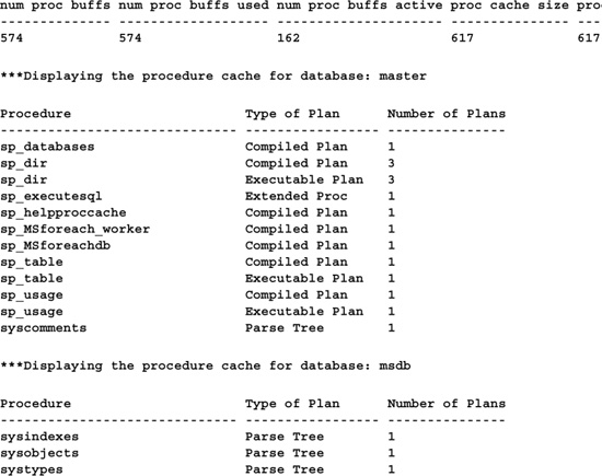
• Use DBCC PROCCACHE to list info about the procedure cache when tuning queries. Use DBCC FREEPROCCACHE to clear the procedure cache in order to keep multiple executions of a given procedure from skewing benchmark results. Use DBCC FLUSHPROCINDB to force the recreation of all procedure execution plans for a given database.
• You can query the syscacheobjects table in the master database to list caching information for procedures, triggers, and other objects. One key piece of information that’s reported by syscacheobjects is the number of plans in the cache for a particular object. This can help you determine whether a plan is being reused when you execute a procedure. Syscacheobjects is a pseudotable—it does not actually exist—the server materializes it each time you query it (you can execute SELECT OBJECTPROPERTY(OBJECT_ID(’syscacheobjects’), ’TableIsFake’) to verify this). Here’s a stored procedure that reports on the procedure cache and queries syscacheobjects for you:
USE master
IF OBJECT_ID(’sp_helpproccache’) IS NOT NULL
DROP PROC sp_helpproccache
GO
CREATE PROCEDURE sp_helpproccache @dbname sysname = NULL,
@procsonly varchar(3)=’NO’,
@executableonly varchar(3)=’NO’
/*
Object: sp_helproccache
Description: Lists information about the procedure cache
Usage: sp_helproccache @dbname=name of database to list; pass ALL to list
all,
@procsonly=[yes|NO] list stored procedures only,
@executableonly=[yes|NO] list executable plans only
Returns: (None)
Created by: Ken Henderson. Email: [email protected]
Version: 1.3
Example: EXEC sp_helpproccache "ALL", @proconly="YES”
Created: 1999-06-02. Last changed: 1999-08-11.
*/
AS
SET NOCOUNT ON
DECLARE @sqlstr varchar(8000)
IF (@dbname=’/?’) GOTO Help
DBCC PROCCACHE
PRINT ’’
SET @sqlstr=
"SELECT LEFT(o.name,30) AS ’Procedure’,
LEFT(cacheobjtype,30) AS ’Type of Plan’,
COUNT(*) AS ’Number of Plans’
FROM master..syscacheobjects c JOIN ?..sysobjects o ON (c.objid=o.id)
WHERE dbid = db_id(’?’)"+
CASE @procsonly WHEN ’YES’ THEN ’ and objtype = "Proc" ’ ELSE ’ ’ END+
CASE @executableonly WHEN ’YES’ THEN
’ and cacheobjtype = "Executable Plan" ’ ELSE ’ ’ END+
"GROUP BY o.name, cacheobjtype
ORDER BY o.name, cacheobjtype”
IF (@dbname=’ALL’)
EXEC sp_MSforeachdb @command1="PRINT ’***Displaying the procedure cache for
database: ?’",
@command2=’PRINT ""’, @command3=@sqlstr
ELSE BEGIN
PRINT ’***Displaying the procedure cache for database: ’+DB_NAME()
PRINT ’’
SET @sqlstr=REPLACE(@sqlstr,’?’,DB_NAME())
EXEC(@sqlstr)
END
RETURN 0
Help:
EXEC sp_usage @objectname=’sp_helproccache’,
@desc=’Lists information about the procedure cache’,
@parameters=’@dbname=name of database to list; pass ALL to list all,
@procsonly=[yes|NO] list stored procedures only,
@executableonly=[yes|NO] list executable plans only’,
@example=’EXEC sp_helpproccache "ALL", @proconly="YES"’,
@author=’Ken Henderson’,
@email=’[email protected]’,
@version=’1’, @revision=’3’,
@datecreated=’6/2/99’, @datelastchanged=’8/11/99’
RETURN -1
GO
EXEC sp_helpproccache ’ALL’

Strive to construct queries that are “SARGable.” A SARG, or search argument, is a clause in a query that the optimizer can potentially use in conjunction with an index to limit the results returned by the query. SARGs have the form:
Column op Constant/Variable
(the terms can be reversed) where Column is a table column; op is one of the following inclusive operators: =,>=,<=, >, <, BETWEEN, and LIKE (some LIKE clauses qualify as SARGs; some don’t—see below for details); and Constant/Variable is a constant value or variable reference.
SARGs can be joined together with AND to form compound clauses. The rule of thumb for identifying SARGs is that a clause can be a useful search argument if the optimizer can detect that it’s a comparison between an index key value and a constant or variable. A clause that compares two columns or one that compares two expressions is not a SARG clause. A common beginner’s error is to wrap a column in a function or expression when comparing it with a constant or variable. This prevents the clause from being a SARG because the optimizer doesn’t know what the expression is actually evaluating—it’s not known until runtime. Here’s an example of such a query.
-- Don’t do this -- Bad T-SQL
SELECT city, state, zip FROM authors
WHERE au_lname+’, ’+au_fname=’Dull, Ann’
city state zip
---------- --------- ----- -----
Palo Alto CA 94301
Better written, this query might look like this:
SELECT city, state, zip
FROM authors
WHERE au_lname=’Dull’
AND au_fname=’Ann’
To see the difference this small change makes, let’s look at the execution plan generated by each. To enable execution plan viewing in Query Analyzer, press Ctrl-K or select Show Execution Plan from the Query menu and run the query. Figure 16.1 shows the execution plan for the first query, and Figure 16.2 shows the plan for the second query.

You can view details for a particular execution plan step by resting your mouse pointer over it. Execution plans read from right to left, so start with the rightmost node and work your way to the left. See the difference? The concatenation of the au_lname and au_fname columns in the first query prevents the use of the aunmind index—whose keys feature both columns. Instead, the first query must use the table’s clustered index, whose key is the au_id column, not terribly useful for locating an author by name (it’s effectively a table scan). By contrast, the second query is able to use the author name index because it correctly avoids confusing the optimizer with unnecessary string concatenation.
Let’s consider some additional queries and determine whether they’re “SARGable.” We’ll begin by adding a few indexes for the sake of comparison. Run the following script to set up some additional secondary indexes:
USE pubs
CREATE INDEX qty ON sales (qty)
CREATE INDEX pub_name ON publishers (pub_name)
CREATE INDEX hirange ON roysched (hirange)
USE Northwind
CREATE INDEX ContactName ON Customers (ContactName)

Here’s a query that selects rows from the pubs sales table based on the qty column:
SELECT *
FROM sales
WHERE qty+1 > 10
Does the WHERE clause contain a SARG? Let’s look at the execution plan (Figure 16.3).
The optimizer has chosen a clustered index scan—essentially a sequential read of the entire table—even though there’s an index on the qty column. Why? Because the qty column in the query is involved in an expression. As mentioned before, enclosing a table column in an expression prevents it from being useful to the optimizer as a SARG. Let’s rewrite the query’s WHERE clause such that the qty column stands alone (Figure 16.4):
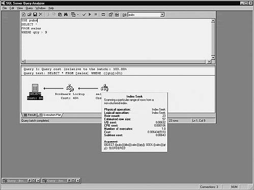
SELECT *
FROM sales
WHERE qty > 9
Since an unfettered qty is now being compared with a constant, the optimizer elects to use the index we added earlier.

Here’s another example (Figure 16.5):
SELECT * FROM authors
WHERE au_lname LIKE ’%Gr%’
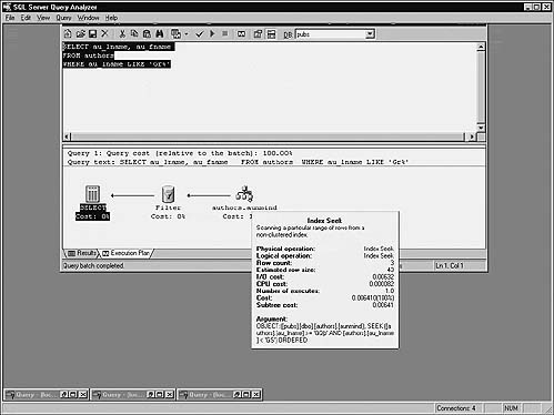
Once again, the optimizer has elected to do a clustered index scan rather than use the nonclustered index that’s built on the au_lname column. The reason for this is simple—it can’t translate the LIKE mask into a usable SARG. Let’s rewrite the query to make it SARGable (Figure 16.6):
SELECT au_lname, au_fname
FROM authors
WHERE au_lname LIKE ’Gr%’

Note
In addition to their obvious syntactical differences, the LIKE masks of the two queries differ functionally as well. Strictly speaking, they don’t ask quite the same question. I’m assuming here that the query author intended to ask for all names beginning with ’Gr’ even though the first mask is prefixed with a wildcard.
Now the optimizer elects to use the nonclustered index on the table that includes au_lname as its high-order key. Internally, the optimizer translates
au_lname LIKE ’Gr%’
to
au_lname > ’GQ_’ AND au_lname < ’GS’

This allows specific key values in the index to be referenced. Value ’GQ_’ can be located in the index (or its closest matching key) and the keys following it read sequentially until ’GS’ is reached. The ’_’ character has the ASCII value of 254, so ’GQ_’ is two values before ’Gr’ followed by any character. This ensures that the first value beginning with ’Gr’ is located.
Let’s look at a similar query with two wildcards:
SELECT *
FROM publishers
WHERE pub_name LIKE ’New%Moon%’
And here’s the execution plan (notice the internal translation of the WHERE clause similar to the previous example) (Figure 16.7).
LIKE expressions that can be restated in terms of “x is greater than value y and less than value z" are useful to the optimizer as SARGs—otherwise they aren’t.
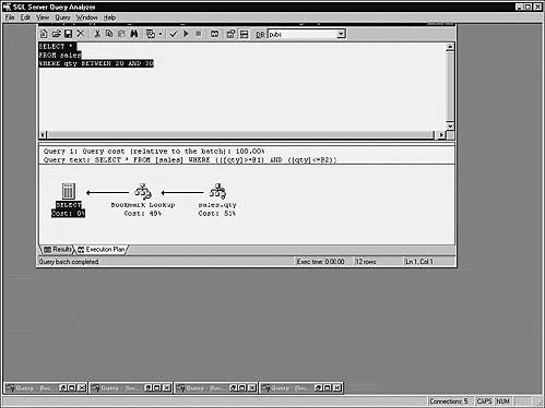
Here’s another query that references the qty column in the pubs sales table (Figure 16.8):
SELECT *
FROM sales
WHERE qty BETWEEN 20 AND 30
Again, the query optimizer translates the WHERE clause into a pair of expressions it finds more useful. It converts the BETWEEN clause into a compound SARG that uses the simpler >= and <= operators to implement BETWEEN’s inclusive search behavior.

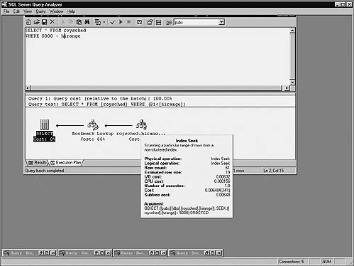
Here’s an example that places the constant on the left of the operator (Figure 16.9):
SELECT * FROM roysched
WHERE 5000 < hirange
As you can see, the ordering of the terms doesn’t matter—the SARG is still correctly identified and matched with the appropriate index.
Let’s look at another query on the sales table. This one involves a search on two columns:
SELECT * FROM sales
WHERE qty > 40 OR stor_id=6380
Prior to SQL Server 7.0, the server would use only one index per table, regardless of how many columns from the same table you listed in the WHERE clause. That’s no longer the case, and, as you can see from the query’s execution plan, the table’s clustered index and the nonclustered index we built on the qty column earlier are used to populate the result set. Since we joined the two SARG clauses via OR, they’re processed in parallel using the appropriate index and then combined using a “hash match” operation just before being returned as a result set (Figure 16.10).
In the past, inequalities were the Achilles heel of the query optimizer—it didn’t know how to translate them into index key values and consequently would perform a full scan of the table in order to service them. That’s still true on some DBMSs but not SQL Server. For example, consider this query:
SELECT *
FROM sales
WHERE qty != 0
Figure 16.11 shows the execution plan we get.

qty !=0
to
qty < 0 OR qty > 0
This allows comparisons with specific index key values and facilitates the use of the index we built earlier, as the execution plan shows.

Here’s an example that filters the result set based on parts of a date column—a common need and an area rife with common pitfalls:
USE Northwind
SELECT * FROM Orders
WHERE DATEPART(mm,OrderDate)=5
AND DATEPART(yy,OrderDate)=1998
AND (DATEPART(dd,OrderDate) BETWEEN 1 AND 3)
This query requests the orders for the first three days of a specified month. Figure 16.12 shows the execution plan it produces.

This execution plan performs a sequential scan of the clustered index and then filters the result according to the WHERE clause criteria. Is the query optimizer able to use any of the WHERE clause criteria as SARGs? No. Once again, table columns are ensconced in expressions—the optimizer has no way of knowing what those expressions actually render. Here’s the query rewritten such that it allows the optimizer to recognize SARGs (Figure 16.13):
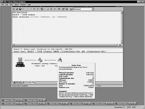
USE Northwind
SELECT * FROM Orders
WHERE OrderDate BETWEEN ’19980501’ AND ’19980503’
As you can see, the optimizer now properly recognizes and uses the SARGs in the WHERE clause to filter the query. It translates the BETWEEN clause into a compound SARG that uses the OrderDate index of the Orders table.
What happens if we want more than three days of data? What if we want the whole month? Here’s the first query rewritten to request an entire month’s worth of data (Figure 16.14):
USE Northwind
SELECT * FROM Orders
WHERE DATEPART(mm,OrderDate)=5
AND DATEPART(yy,OrderDate)=1998
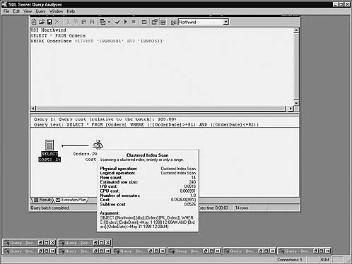
And here’s the improved version of the query, similarly modified (Figure 16.15):
USE Northwind
SELECT * FROM Orders
WHERE OrderDate BETWEEN ’19980501’ AND ’19980531’

Interestingly, the improved query now scans the clustered index as well. Why? The amount of data being returned is the key. The optimizer has estimated that it’s less expensive to scan the entire table and filter results sequentially than to use the nonclustered index because each row located via the index must then be looked up in the clustered index (or underlying table if no clustered index exists) in order to retrieve the other columns the query requests.
The step in the execution plan where this occurs is called the “Bookmark lookup” step (see Figure 16.13 for an example). An execution plan that locates rows using a nonclustered index must include a Bookmark lookup step if it returns columns other than those in the index. In this case, the optimizer has estimated that the overhead of this additional step is sufficient to warrant a full clustered index scan. In the original query, this step accounted for 80% of the execution plan’s total work, so this makes sense. We’ve now multiplied the number of rows being returned several times over, so this step has become so lengthy that it’s actually more efficient just to read the entire table.
There are a couple of ways around this. We’ve already explored one of them—returning less data. In fact, the threshold at which the optimizer decides it’s more efficient to perform a sequential scan is at five days’ worth of Orders data—returning five or more days results in a clustered index scan. Another way around this would be to eliminate the Bookmark lookup step altogether by satisfying the query with a nonclustered index. To do this, we’d either have to create a nonclustered index containing the columns we want to return (the wider the index key becomes, the more expensive using it becomes in terms of I/O) or narrow the columns we request to those already in a nonclustered index. In this case, that would mean requesting only the OrderDate column from the table since that’s the lone key column of the nonclustered index we’re using (by virtue of the WHERE clause criteria). Here’s the query revised to request only the OrderDate column and its accompanying execution plan (Figure 16.16):
USE Northwind
SELECT OrderDate FROM Orders
WHERE OrderDate BETWEEN ’19980501’ AND ’19980531’
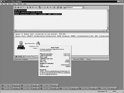
Now, neither the clustered index nor the Bookmark lookup step is needed. As mentioned earlier, this is called index covering, meaning that the nonclustered index covers the query—it’s able to satisfy it—without referencing the underlying table or its clustered index.
Practically speaking, it’s pretty rare that you’ll find a nonclustered index whose key columns satisfy a query completely. However, you’ll often find that adding a column or two to the nonclustered index used by a query allows it to cover the query without becoming excessively expensive. Keep in mind that widening nonclustered index key columns results in slower updates, because they must be kept up to date, and slower query processing, because they’re physically larger—they require more I/O and more memory to process.
Table 16.1 lists some examples of SARGable and non-SARGable clauses.

Especially among developers new to relational databases, there’s sometimes a temptation to attribute poor database design to “denormalization for performance.” You can’t know for certain whether denormalizing a database is necessary until you’ve first normalized it and tested performance thoroughly. Even then, denormalizing shouldn’t be your first option—it should be near the bottom of the list. I wouldn’t recommend denormalization as the first method of fixing a performance problem any more than I’d recommend brain surgery for a headache. As a rule, garden-variety applications’ development does not require database denormalization. If it did, the database design standards that have been forged and refined over the last thirty years wouldn’t be worth much—what good is a standard if you have to break it in order to do anything useful?
That said, denormalization is a fairly common method of improving query performance—especially in high-performance and high-throughput systems. Eliminating a single join operation from a query that processes millions of rows can yield real dividends.
Understand that there’s no absolute standard of measurement by which a database either is or isn’t normalized. There are different degrees of normalization, but even the best database designers build databases that fail to measure up in some way to someone else’s concept of normalization.
• Know your database. Be sure you understand how it’s organized from a logical standpoint, and be sure you know how applications use it. Have a good understanding of the database’s data integrity setup. Introducing redundant data into the system makes maintaining data integrity more difficult and more expensive in terms of performance. It’s therefore crucial to understand the frequency of data modifications. If the database serves a high-throughput OLTP application, you may find that the performance gains you achieved through denormalization are offset by the performance problems its creates in maintaining data integrity.
• Don’t denormalize the entire database at once. Start small, working with logically separable pieces.
• Ascertain early on whether computed or contrived columns would address your performance needs. You may find that SQL Server’s computed columns provide the performance your app requires without having to resort to large-scale denormalization.
• Become intimate with the data volume and the transaction types underlying the parts of your application having performance problems. You will probably find that you can further tune your queries or the server and resolve those problems without having to redesign the database.
• Become acquainted with the material resources of your server machine. Increasing the physical memory in the machine or the amount that’s allocated to the SQL Server process may improve query performance dramatically. Adding or upgrading processors may help—especially if you have key queries that are CPU-bound. The biggest gains in terms of system performance usually come from hard drive–related optimizations. Using a speedier hard drive or more of them may improve performance by orders of magnitude. For example, you may find that using RAID in conjunction with filegroups can resolve your performance problems without having to denormalize.
A number of techniques that you can use to denormalize a database and hopefully improve performance exist:
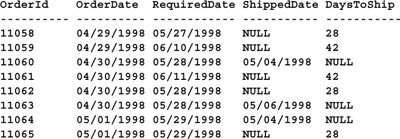
A contrived or virtual column is one that’s composed of the values from other columns. SQL Server includes direct support for contrived columns through its computed column support. Setting up a computed column saves you from having to include its underlying expression each time you query the table. It’s syntactically more compact and makes the expression’s result readily available to anyone who uses the table. You define computed columns with the CREATE TABLE or ALTER TABLE command. Here’s an example:
USE Northwind
GO
ALTER TABLE Orders ADD DaysToShip AS CASE WHEN ShippedDate IS NULL THEN
DATEDIFF(dd,OrderDate,RequiredDate) ELSE NULL END
GO
SELECT OrderId, CONVERT(char(10),OrderDate,101) AS OrderDate,
CONVERT(char(10),RequiredDate,101) AS RequiredDate,
CONVERT(char(10),ShippedDate,101) AS ShippedDate,
DaysToShip FROM Orders
GO
ALTER TABLE Orders DROP COLUMN DaysToShip
GO
(Results abridged)
A common denormalization technique is to maintain multiple copies of the same data. For example, you may find that it’s worthwhile to look up and store join values in advance. This cuts down on the work necessary to return useful information when you query a table. A variation on this duplicates foreign key values so that they don’t have to be referenced across tables. Of course, you’ll want to be careful with this because it adds additional overhead to maintaining data integrity. The more copies of data you have, the more work required to keep it up to date and the more likely a mishap can compromise database integrity. The corollary to this is the essence of the relational model: The fewer copies of nonkey data you have, the easier it is to maintain and the less likely its integrity is to be damaged in the event of problems.
Here’s an example that adds columns for the first and last names of authors to the pubs titleauthor table:

By adding these redundant columns to titleauthor, we’ve eliminated one of the joins that must be performed in order to return useful information from the table. For a query processing millions of rows, this can make a significant difference in performance. Of course, a mechanism similar to the UPDATE featured in the example must be used to ensure that these redundant values are properly maintained.
An increasingly common method of denormalizing for performance involves the creation of summary tables—tables that summarize detail data from other tables. The technique has become so popular, in fact, that some DBMS vendors offer built-in support for summary tables.
Building a summary table typically consists of running a popular query (that perhaps takes an extended period of time to run) ahead of time and storing its results in a summary table. When applications need access to the data, they access this static table. Then—during off-peak periods or whenever it’s convenient—the summary query can be rerun and the table updated with the latest info. This works well and is a viable alternative to executing lengthy queries repetitively.
One problem with this approach is in administration. Setting up a summary table counterpart for a detail table doubles the administrative work on that table. If you had ten stored procedures on the original table, you are likely to need twenty now. Everything you did for the detail table in terms of administration must now be done redundantly—all triggers, constraints, etc. must be maintained in two places now rather than one. The more summary tables you have, the more headaches you have.
An option that solves the administrative dilemma while providing the query performance gains of summary tables is what I call inline summarization. Inline summarization involves changing the original detail table slightly so that it can store summary as well as detail data, then summarizing a portion of it and inserting that summary data back into the table itself, optionally removing or archiving the original detail rows. One of the benefits of this approach is that summary and detail data can be easily queried together or separately—in fact, queries over the table normally don’t know whether they’re working with detail or summary data. Subtle clues can indicate which rows are summary rows, but they are otherwise indistinguishable from their detail siblings. Note that, strictly speaking, if you remove the detail data, you also avoid the problems that accompany keeping redundant data. Another benefit of this approach is that you don’t have the redundant administration hassles that accompany the separate table approach. All the foreign key references, triggers, constraints, views, query batches, and stored procedures that worked with the detail data work automatically with summary data, too.
This is best explored by way of example. Here’s a query that performs inline summarization on the Orders table in the Northwind sample database:
USE Northwind
GO
ALTER TABLE Orders ADD NumberOfOrders int DEFAULT 1 -- Add summary column
GO
UPDATE Orders SET NumberOfOrders=DEFAULT -- Force current rows to contain DEFAULT value
GO
-- Insert summary info
INSERT Orders (CustomerID, EmployeeID, OrderDate, RequiredDate, ShippedDate,
ShipVia, Freight, ShipName, ShipAddress, ShipCity,
ShipRegion, ShipPostalCode, ShipCountry, NumberOfOrders)
SELECT NULL, EmployeeID, CONVERT(char(6), OrderDate, 112)+’01’,
’19000101’, ’19000101’,1,0,’’,’’,’’,’’,’’,’’,COUNT(*) -- Summarize rows
FROM Orders
WHERE OrderDate < ’19980101’
GROUP BY EmployeeID, CONVERT(char(6), OrderDate, 112)+’01’
-- Delete Order Details rows corresponding to summarized rows
DELETE d
FROM [Order Details] d JOIN Orders o ON d.OrderID=o.OrderID
WHERE o.OrderDate <’19980101’ AND RequiredDate > ’19000101’
-- Use RequiredDate to leave summary rows
-- Delete nonsummary versions of rows that were summarized
DELETE Orders
WHERE OrderDate < ’19980101’ AND RequiredDate > ’19000101’
This query begins by adding a new column to the Orders table, NumberOfOrders. In the past, determining the number of orders on file involved using COUNT(*). Inline summarization changes that. It uses NumberOfOrders to indicate the number of orders a given row represents. In the case of detail tables, this is always “1”—hence the DEFAULT constraint. In the case of summary rows, this could be any number up to the maximum int can store. So, to aggregate the number of orders, we simply sum the NumberOfOrders column. Regardless of whether the rows summed are detail or summary rows, this works as we expect.
What this means is that instead of running this query to list the number of orders per month:


It’s perhaps helpful to look at the data itself. Here’s a small sample of it:

Notice that the CustomerID column is NULL in summary rows because we summed on EmployeeID and OrderMonth. This is one way to distinguish summary rows from detail rows. Another way is to inspect the RequireDate column—it’s always set to 01/01/1900—SQL Server’s base date—in summary rows.
Since SQL Server uses a fixed database page size of 8KB and a single row cannot span pages, the number of rows that will fit on a page is determined by row width. The wider a row, the fewer rows that fit on each page. Physically splitting a table into multiple tables allows more rows to fit on a page, potentially increasing query performance. Here’s an example that vertically partitions the Orders table in the Northwind sample database:
SET NOCOUNT ON
USE Northwind
BEGIN TRAN -- So we can undo all this
DECLARE @pagebin binary(6), @file int, @page int
-- Get the first page of the table (usually)
SELECT TOP 1 @pagebin=first
FROM sysindexes
WHERE id=OBJECT_ID(’Orders’)
ORDER BY indid
-- Translate first into a file and page number
EXEC sp_decodepagebin @pagebin, @file OUT, @page OUT
-- Show the first file and page in the table
-- Look at the m_slotCnt column in the page header to determine
-- the number of row/page for this page.
DBCC TRACEON(3604)
PRINT CHAR(13)
PRINT ’***Dumping the first page of Orders BEFORE the partitioning’
DBCC PAGE(’Northwind’,@file,@page,0,1)
-- Run a query so we can check the cost of the query
-- before the partitioning
SELECT *
INTO #ordertmp1
FROM Orders
-- Now partition the table vertically into two separate tables
-- Create a table to hold the primary order information
SELECT OrderID, CustomerID, EmployeeID, OrderDate, RequiredDate
INTO OrdersMain
FROM Orders
-- Add a clustered primary key
ALTER TABLE OrdersMain ADD CONSTRAINT PK_OrdersMain PRIMARY KEY (OrderID)
-- Create a table that will store shipping info only
SELECT OrderID, Freight, ShipVia, ShipName, ShipAddress, ShipCity, ShipRegion,
ShipPostalCode, ShipCountry
INTO OrdersShipping
FROM Orders
-- Add a clustered primary key
ALTER TABLE OrdersShipping ADD CONSTRAINT PK_OrdersShipping PRIMARY KEY (OrderID)
-- Now check the number of rows/page in the first of the new tables.
-- Vertically partitioning Orders has increased the number of rows/page
-- and should speed up queries
SELECT TOP 1 @pagebin=first
FROM sysindexes
WHERE id=OBJECT_ID(’OrdersMain’)
ORDER BY indid
EXEC sp_decodepagebin @pagebin, @file OUT, @page OUT
PRINT CHAR(13)
PRINT ’***Dumping the first page of OrdersMain AFTER the partitioning’
DBCC PAGE(’Northwind’,@file,@page,0,1)
-- Run a query so we can check the cost of the query
-- after the partitioning
SELECT *
INTO #ordertmp2
FROM OrdersMain
-- Check the number of rows/page in the second table.
SELECT TOP 1 @pagebin=first
FROM sysindexes
WHERE id=OBJECT_ID(’OrdersShipping’)
ORDER BY indid
EXEC sp_decodepagebin @pagebin, @file OUT, @page OUT
PRINT CHAR(13)
PRINT ’***Dumping the first page of OrdersShipping AFTER the partitioning’
DBCC PAGE(’Northwind’,@file,@page,0,1)
DBCC TRACEOFF(3604)
DROP TABLE #ordertmp1
DROP TABLE #ordertmp2
GO
ROLLBACK TRAN -- Undo it all
***Dumping the first page of Orders BEFORE the partitioning
PAGE:
BUFFER:
BUF @0x11B3B000
---------------
bpage = 0x1FD90000 bhash = 0x00000000 bpageno = (1:143)
bdbid = 6 breferences = 8 bkeep = 1
bstat = 0x9 bspin = 0 bnext = 0x00000000
PAGE HEADER:
Page @0x1FD90000
----------------
m_pageId = (1:143) m_headerVersion = 1 m_type = 1
m_typeFlagBits = 0x0 m_level = 0 m_flagBits = 0x0
m_objId = 357576312 m_indexId = 0 m_prevPage = (0:0)
m_nextPage = (1:291) pminlen = 58 m_slotCnt = 42
m_freeCnt = 146 m_freeData = 7962 m_reservedCnt = 0
m_lsn = (18:151:6) m_xactReserved = 0 m_xactId = (0:0)
m_ghostRecCnt = 0 m_tornBits = 81921
GAM (1:2) ALLOCATED, SGAM (1:3) NOT ALLOCATED, PFS (1:1) 0x60 MIXED_EXT ALLOCATED
0_PCT_FULL
DBCC execution completed. If DBCC printed error messages, contact your system
administrator.
***Dumping the first page of OrdersMain AFTER the partitioning
PAGE:
BUFFER:
BUF @0x11B37EC0
---------------
bpage = 0x1FC06000 bhash = 0x00000000 bpageno = (1:424)
bdbid = 6 breferences = 0 bkeep = 1
bstat = 0x9 bspin = 0 bnext = 0x00000000
PAGE HEADER:
Page @0x1FC06000
----------------
m_pageId = (1:424) m_headerVersion = 1 m_type = 1
m_typeFlagBits = 0x0 m_level = 0 m_flagBits = 0x4
m_objId = 2005582183 m_indexId = 0 m_prevPage = (0:0)
m_nextPage = (1:425) pminlen = 38 m_slotCnt = 188
m_freeCnt = 12 m_freeData = 7804 m_reservedCnt = 0
m_lsn = (28:144:24) m_xactReserved = 0 m_xactId = (0:0)
m_ghostRecCnt = 0 m_tornBits = 0
GAM (1:2) ALLOCATED, SGAM (1:3) NOT ALLOCATED, PFS (1:1) 0x40 ALLOCATED 0_PCT_FULL
DBCC execution completed. If DBCC printed error messages, contact your system
administrator.
***Dumping the first page of OrdersShipping AFTER the partitioning
PAGE:
BUFFER:
BUF @0x11B49E80
---------------
bpage = 0x20504000 bhash = 0x00000000 bpageno = (1:488)
bdbid = 6 breferences = 0 bkeep = 1
bstat = 0x9 bspin = 0 bnext = 0x00000000
PAGE HEADER:
Page @0x20504000
----------------
m_pageId = (1:488) m_headerVersion = 1 m_type = 1
m_typeFlagBits = 0x0 m_level = 0 m_flagBits = 0x0
m_objId = 2037582297 m_indexId = 0 m_prevPage = (0:0)
m_nextPage = (1:489) pminlen = 12 m_slotCnt = 55
m_freeCnt = 43 m_freeData = 8039 m_reservedCnt = 0
m_lsn = (28:179:24) m_xactReserved = 0 m_xactId = (0:0)
m_ghostRecCnt = 0 m_tornBits = 0
GAM (1:2) ALLOCATED, SGAM (1:3) NOT ALLOCATED, PFS (1:1) 0x40 ALLOCATED 0_PCT_FULL
The steps this query goes through are as follows:
1. Start a transaction so that all changes can be rolled back when we’re done.
2. Show the first page of the Orders table as it appears before we partition it. This tells us how many rows are being stored on the page (see the m_slotcnt field in the page header).
3. Run a query that traverses the entire table so that we can compare the costs of querying the data before and after partitioning.
4. Partition Orders into two news tables using SELECT...INTO. Put primary order-related columns in one table; put shipping-related columns in the other.
5. Show the first page of the first new table. This tells us how many rows are being stored on the first page of the new table.
6. Run the earlier query against the first of the new tables so we can compare query costs.
7. Dump the first page of the second new table. This tells us how many rows fit on its first page.
8. Drop the temporary tables created by the cost queries.
9. Roll back the transaction.
When you run the query, inspect the m_slotcnt field in the page header of each set of DBCC PAGE output. This field indicates how many row slots there are on the listed page. You’ll notice that it increases substantially from the original Orders table to the OrdersMain table. In fact, it should be roughly four times as high in the new table. What does this mean? It means that a query retrieving rows from OrdersMain will be roughly four times more efficient than one pulling them from Orders. Even if these pages are in the cache, this could obviously make a huge difference.
Understand that the actual number of rows on each page is not constant. That is, even though the first page of the new table may hold, say, 100 rows, the second page may not. This is due to a number of factors. First, SQL Server doesn’t maintain the table’s FILLFACTOR over time. Data modifications can change the number of rows on a given page. Second, if a table contains variable-length columns, the length of each row can vary to the point of changing how many rows fit on a given page. Also, the default FILLFACTOR (0) doesn’t force pages to be completely full—it’s not the same as a FILLFACTOR of 100. A FILLFACTOR of 0 is similar to 100 in that it creates clustered indexes with full data pages and nonclustered indexes with full leaf pages. However, it differs in that it reserves space in the upper portion of the index tree and in the non-leaf-level index pages for the maximum size of one index entry.
This query makes use of the sp_decodepagebin stored procedure. The sp_decodepagebin procedure converts binary file/page numbers such as those in the first, root, and FirstIAM columns of the sysindexes system table to integers that can be used with DBCC PAGE. When passed a binary(6) value, like those in sysindexes, it returns two output parameters containing the file and page number encoded in the value. Here’s its source code:
USE master
IF OBJECT_ID(’sp_decodepagebin’) IS NOT NULL
DROP PROC sp_decodepagebin
GO
CREATE PROC sp_decodepagebin @pagebin varchar(12), @file int=NULL OUT,
@page int=NULL OUT
/*
Object: sp_decodepagebin
Description: Translates binary file/page numbers (like those in the sysindexes
root, first, and FirstIAM columns) into integers
Usage: sp_decodepagebin @pagebin=binary(6) file/page number, @file=OUTPUT parm
for file number, @page=OUTPUT parm for page number
Returns: (None)
Created by: Ken Henderson. Email: [email protected]
Version: 1.2
Example: EXEC sp_decodepagebin "0x050000000100", @myfile OUT, @mypage OUT
Created: 1999-06-13. Last changed: 1999-08-05.
*/
AS
DECLARE @inbin binary(6)
IF (@pagebin=’/?’) GOTO Help
SET @inbin=CAST(@pagebin AS binary(6))
SELECT @file=(CAST(SUBSTRING(@inbin,6,1) AS
int)*POWER(2,8))+(CAST(SUBSTRING(@inbin,5,1) AS int)),
@page=(CAST(SUBSTRING(@inbin,4,1) AS int)*POWER(2,24)) +
(CAST(SUBSTRING(@inbin,3,1) AS int)*POWER(2,16)) +
(CAST(SUBSTRING(@inbin,2,1) AS int)*POWER(2,8)) +
(CAST(SUBSTRING(@inbin,1,1) AS int))
from sysindexes
RETURN 0
Help:
EXEC sp_usage @objectname=’sp_decodepagebin’,
@desc=’Translates binary file/page numbers (like those in the sysindexes
root, first, and FirstIAM columns) into integers’,
@parameters=’@pagebin=binary(6) file/page number, @file=OUTPUT parm for file number,
@page=OUTPUT parm for page number’,
@example=’EXEC sp_decodepagebin "0x050000000100", @myfile OUT, @mypage OUT’,
@author=’Ken Henderson’,
@email=’[email protected]’,
@version=’1’, @revision=’2’,
@datecreated=’6/13/99’, @datelastchanged=’8/5/99’
RETURN –1
This procedure is necessary because the first, root, and FirstIAM pages are not useful in their native format. We need to access first in order to access the table’s starting page (though first isn’t guaranteed to reference the table’s initial page by the server, it’s unfortunately the best access we have). In order to convert the binary(6) value that’s stored in first into a usable file and page number, we need to swap the bytes in the number and then convert the values from hexadecimal to decimal. Once swapped, the initial two bytes of the first column reference its page; the last four identify its page number. By using sp_decodepagebin, we’re spared the details of producing these.
The example code executed a SELECT * query before and after the table partitioning in order to test the effect of the partitioning on query costing. Let’s look at the execution plan of the before and after instances of the query in Figures 16.17 and 16.18.
The most striking difference between the two execution plans is the estimated row size. It drops from 240 in the first query to 41 in the second. Naturally, this means that more rows fit on a given page and more will be retrieved with each page read.

Despite having tuned a given table thoroughly, you may find that it’s just too large to support the type of performance you need. As rows are added to a table, the infrastructure required to support it grows in size. Eventually, it gets so large that index navigation alone is an expensive and time-consuming proposition. Traversing an index B-tree that contains millions of keys can require more time than accessing the data itself.
One answer to this is to partition the table horizontally—to break it into multiple tables based on the value of some column or columns. Then, the number of rows any one query will have to navigate is far less.
Horizontal partitioning is especially handy when a subset of a table is considerably more active than the rest of the table. By putting it in its own partition, you allow queries that reference it to avoid wading through lots of data they don’t need.
Unlike vertically partitioned tables, horizontal partitions contain identical columns. Here’s an example that horizontally partitions the Orders table in the Northwind sample database by month based on the OrderDate column:
USE Northwind
BEGIN TRAN -- So we can undo all this

-- Drop the index so we can see the effects of paritioning more easily
DROP INDEX Orders.OrderDate
SELECT *
INTO P199701_Orders
FROM Orders
WHERE OrderDate BETWEEN ’19970101’ AND ’19970131’
SELECT *
INTO P199702_Orders
FROM Orders
WHERE OrderDate BETWEEN ’19970201’ AND ’19970228’
SELECT *
INTO P199703_Orders
FROM Orders
WHERE OrderDate BETWEEN ’19970301’ AND ’19970331’
SELECT *
INTO P199704_Orders
FROM Orders
WHERE OrderDate BETWEEN ’19970401’ AND ’19970430’
SELECT *
INTO P199705_Orders
FROM Orders
WHERE OrderDate BETWEEN ’19970501’ AND ’19970531’
SELECT *
INTO P199706_Orders
FROM Orders
WHERE OrderDate BETWEEN ’19970601’ AND ’19970630’
SELECT *
INTO P199707_Orders
FROM Orders
WHERE OrderDate BETWEEN ’19970701’ AND ’19970731’
SELECT *
INTO P199708_Orders
FROM Orders
WHERE OrderDate BETWEEN ’19970801’ AND ’19970831’
SELECT *
INTO P199709_Orders
FROM Orders
WHERE OrderDate BETWEEN ’19970901’ AND ’19970930’
SELECT *
INTO P199710_Orders
FROM Orders
WHERE OrderDate BETWEEN ’19971001’ AND ’19971031’
SELECT *
INTO P199711_Orders
FROM Orders
WHERE OrderDate BETWEEN ’19971101’ AND ’19971130’
SELECT *
INTO P199712_Orders
FROM Orders
WHERE OrderDate BETWEEN ’19971201’ AND ’19971231’
-- Now let’s run a couple queries to see the effects of the partitioning
SELECT CONVERT(char(6), OrderDate, 112) OrderMonth, COUNT(*) NumOrders
FROM Orders
WHERE OrderDate BETWEEN ’19970701’ AND ’19970731’
GROUP BY CONVERT(char(6), OrderDate, 112)
ORDER BY OrderMonth
ALTER TABLE P199707_Orders ADD CONSTRAINT PK_P199707_Orders PRIMARY KEY (OrderID)
SELECT CONVERT(char(6), OrderDate, 112) OrderMonth, COUNT(*) NumOrders
FROM P199707_Orders
WHERE OrderDate BETWEEN ’19970701’ AND ’19970731’
GROUP BY CONVERT(char(6), OrderDate, 112)
ORDER BY OrderMonth
OrderMonth NumOrders
---------- -----------
199707 33
OrderMonth NumOrders
---------- -----------
199707 33
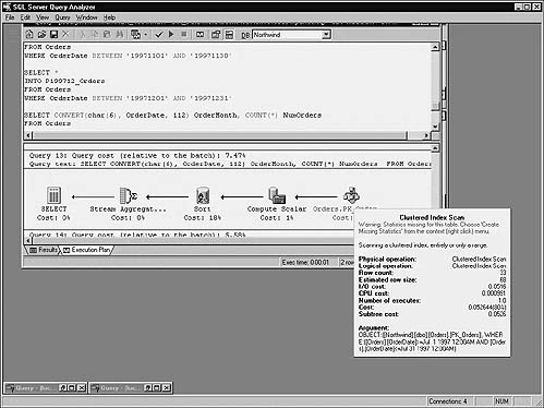
To see the effect partitioning the table has had on performance, let’s examine the execution plans of the two grouped SELECTs in the query—Figures 16.19 and 16.20.
The query against the partitioned table is 28% more efficient in terms of I/O cost and 89% more efficient in terms of CPU cost. Obviously, traversing a subset of a table is quicker than traversing the entire table.
Among the drawbacks of horizontal partitioning is increased query complexity. Queries that span more than one partition become linearly more complicated. You can alleviate some of this by using views to merge partitions via UNIONs, but this is only marginally effective. Some degree of additional complexity is unavoidable. Also, self-referencing constraints are at a disadvantage when horizontal partitions are present. If a table needs to reference itself to check the validity of a value, the presence of partitions may force it to have to check several other tables.

One of the strengths of modern relational DBMSs is server-based query optimization. It’s an area where client/server systems have a distinct advantage over flat-file databases. Without a server, there’s little opportunity for optimizing queries submitted by applications, especially multiuser applications. For example, there’s no chance of reusing the execution plan of a query run by one user with one run by another user. There’s no opportunity to cache database objects accessed by multiple users in a manner beyond simplistic file system–based caching because nothing but the database drivers knows anything about the database. To the operating system, it’s just another file or files. To the application, it’s a resource accessed by way of a special driver, usually a DLL. In short, no one’s in charge—no one’s minding the store as far as making sure access to the database is consistent and efficient across all the clients using it.
Client/server DBMSs have changed this by making the server an equal partner with the developer in ensuring database access is as efficient as possible. The science behind query optimization has evolved over the years to the point that the optimizer is usually able to tune a query better and more quickly than a human counterpart. A modern optimizer can leverage one of the things computers do best—iteration. It can quickly loop through an assortment of potential query solutions in order to select the best one.
DBMSs take a variety of approaches to optimizing queries. Some optimize based on heuristics—internally reordering and reorganizing queries based on a predefined set of algebraic rules. Query trees are dissected, and associative and commutative rules are applied in a predetermined order until a plan for satisfying the entire query emerges.
Some DBMSs optimize queries based on syntactic elements. This places the real burden of optimization on the user because WHERE clause predicates and join criteria are not reordered—they generate the same execution plan with each run. Because the user becomes the real optimizer, intimate knowledge of the database is essential for good query performance.
Semantic optimization is a theoretical technique that assumes the optimizer knows the database schema and can infer optimization potential through constraint definitions. Several vendors are exploring this area of query optimization as a means of allowing a database designer or modeler a direct means of controlling the optimization process.
The most prevalent means of query optimization, and, I think, the most effective, is cost-based optimization. Cost-based optimization weighs several different methods of satisfying a query against one another and selects the one that will execute in the shortest time. A cost-based optimizer bases this determination on estimates of I/O, CPU utilization, and other factors that affect query performance. This is the approach that SQL Server takes, and its implementation is among the most advanced in the industry.
I’ve already touched briefly on the query optimizer and some of its features elsewhere in this chapter, but I think it’s essential to have a good understanding of how it works in order to write optimal T-SQL code and to tune queries properly.
The optimizer goes through several steps in order to optimize a query. It analyzes the query, identifying SARGs and OR clauses, locating joins, etc. It compares different ways of performing any necessary joins and evaluates the best indexes to use with the query. Since the optimizer is cost-based, it selects the method of satisfying the query with the least cost. Usually, it makes the right choice, but sometimes it needs a little help.
Releases 7.0 and later of SQL Server support join types beyond the simple nested loop (or nested iteration) joins of earlier releases. This flexibility allows the optimizer to find the best way of linking one table with another using all the information at its disposal.
Nested loop joins consist of a loop within a loop. They designate one table in the join as the outer loop and the other as the inner loop. For each iteration of the outer loop, the entire inner loop is traversed. This works fine for small to medium-sized tables, but as the loops grow larger, this strategy becomes increasingly inefficient. Figure 16.21 illustrates a nested loop query and its execution plan.
Merge joins perform much more efficiently with large data sets than nested loop joins. A row from each table in the join is retrieved and compared. Both tables must be sorted on the merge column for the join to work. The optimizer usually opts for a merge join when working with a large data set and when the comparison columns in both tables are already sorted. Figure 16.22 illustrates a query that the optimizer processes using a merge join.

Hash joins are also more efficient with large data sets than nested loop joins. Additionally, they work well with tables that are not sorted on the merge column(s). The server performs hash joins by hashing the rows from the smaller of the two tables (designated the “build” table), inserting them into a hash table, processing the larger table (the “probe” table) a row at a time, and scanning the hash table for matches. Because the smaller of the two tables supplies the values in the hash table, the table size is kept to a minimum, and because hashed values rather than real values are used, comparisons can be made between the tables very quickly.
Hash joins are a variation on the concept of hashed indexes that have been available in a handful of advanced DBMS products for several years. With hashed indexes, the hash table is stored permanently—it is the index. Data is hashed into slots that have the same hashing value. If the index has a unique contiguous key, what is known as a minimal perfect hashing function exists—every value hashes to its own slot and there are no gaps between slots in the index. If the index is unique but noncontiguous, the next best thing—a perfect hashing function—can exist wherein every value hashes to its own slot, but potentially there are gaps between them. Figure 16.23 illustrates a hash join.
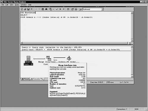
In addition to identifying search arguments and using indexes to service them, the query optimizer can make use of indexes in other ways to streamline query processing. A number of these are made possible by the optimizer’s ability to make use of multiple indexes on the same table.
As mentioned elsewhere in this chapter, index covering is the process whereby the optimizer uses a nonclustered index to satisfy a query rather than referencing the underlying table or clustered index. It requires that the columns requested by the query exist as keys in a nonclustered index. An execution plan that uses a nonclustered index to retrieve data but does not include a Bookmark lookup step is making use of index covering. SQL Server can join multiple nonclustered indexes to create covered indexes on the fly. This is often faster than using the indexes separately and certainly quicker than sequentially scanning the table itself. Figure 16.24 shows a query that the optimizer translates into a join between two nonclustered indexes.
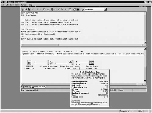
SQL Server’s ability to join nonclustered indexes in this fashion has some ramifications for physical database design. Prior to the advent of index joins, the common technique for setting up index covering was to add a column or two to an existing index in order to allow it to cover a given query or queries. Now that the optimizer can join indexes, it may be more sensible to split these keys into multiple indexes and allow the optimizer to join them as necessary. This allows the optimizer to use them individually as well, which wouldn’t be the case with a compound key. This isn’t to say that you should abandon compound index keys altogether, but splitting them into separate indexes is certainly something to consider.
Similar to index joins is the optimizer’s ability to merge and intersect indexes. This allows it to merge the matching keys in multiple indexes into a set of key values that it may then look up in the clustered index or underlying table in order to retrieve columns not found in the indexes. Figure 16.25 illustrates an index merge/intersection query and execution plan.
Notice that the execution plan includes a Bookmark lookup step. This means that the query isn’t being covered by nonclustered indexes. They are, however, intersected to help service it.

In addition to the data warehousing and OLAP tools that ship with SQL Server, the query optimizer can recognize star schema layouts and perform special optimizations for queries that join fact and dimension tables. Since dimension tables tend to be microscopic compared with fact tables, the query optimizer can generate an execution plan that first cross-joins the dimension tables in a query with each other and then joins the result with the fact table. The end result is a smaller number of joins than with traditional methods of combining these types of tables.
This is best understood by way of example. For the sake of discussion, assume we have three tables—two dimension tables and one fact table. The dimension tables have ten rows each, and the fact table has a million rows. If you join the fact table to the two dimension tables with inner joins and the optimizer performs no additional optimizations, two million joins will be performed (one million for the join between the fact table and the first dimension table and one million for the join with the second dimension table). If, instead, you cross-join the two dimension tables, then join the fact table with the result, you reduce the number of joins by nearly half:

10 × 10 dimension rows 5 100 joins
+ 1 1,000,000 joins between the fact table and the dimension composite
= 1,000,100 total joins
The following SQL script illustrates a typical star schema join. It first constructs the dimension and fact tables described earlier and then joins the fact table with the two dimension tables.
Note
Don’t run this query with Show Execution Plan enabled in Query Analyzer—each row insertion will get its own section in the graphical execution plan, which will take an eternity to run and not be terribly useful. If you want to see the join query’s execution plan for yourself, highlight the portion of the script up to the join and press Ctrl-E in Query Analyzer to run it. This will create the tables and populate them with data. Next, press Ctrl-K to turn on the graphical execution plan display; highlight the join itself and run it.
SET NOCOUNT ON
CREATE TABLE #dim1 (dim1 int identity PRIMARY KEY, dim1val int)
CREATE TABLE #dim2 (dim2 int identity PRIMARY KEY, dim2val int)
CREATE TABLE #facttable (k1 int identity PRIMARY KEY, dim1 int, dim2 int)
DECLARE @loop INT
SET @loop=1
WHILE @loop<=10 BEGIN
INSERT #dim1 VALUES (@loop*50)
INSERT #dim2 VALUES (@loop*25)
SET @loop=@loop+1
END
SET @loop=1
WHILE @loop<=1000000 BEGIN
INSERT #facttable VALUES ((@loop / 100000)+1,10-(@loop / 100000))
SET @loop=@loop+1
END
SELECT COUNT(*)
FROM #facttable f JOIN #dim1 d ON (f.dim1=d.dim1)
JOIN #dim2 i ON (f.dim2=i.dim2)
When the fact table in a star schema relationship contains indexes on the dimension columns used in a join, the optimizer will use those indexes to perform index intersections with the dimension tables. Each dimension table will be joined with an appropriate index on the fact table, and the results of those joins will be intersected before retrieving rows from the fact table. This strategy allows the optimizer to return rows from the fact table when it’s most efficient to do so—after membership in the result set has been pared down by the index intersections.
The normal order of events when GROUP BY is present in a query containing joins is to perform the joins before grouping the data. Sometimes, however, it’s faster to group the data first, especially when working with a huge number of rows that will be coalesced into a relatively small number of groups. In the past, Transact-SQL developers had to perform this optimization by hand, usually via a stored procedure and some temporary tables. Now, the optimizer can potentially recognize situations where grouping first would be beneficial and act accordingly.
The optimizer can detect when predicate clauses are associative and eliminate unnecessary join steps. Here’s a query that illustrates:

SET NOCOUNT ON
CREATE TABLE #tmp1 (k1 int identity PRIMARY KEY)
CREATE TABLE #tmp2 (k1 int identity PRIMARY KEY)
CREATE TABLE #tmp3 (k1 int identity PRIMARY KEY)
DECLARE @loop int
SET @loop=1
WHILE @loop<=10 BEGIN
INSERT #tmp1 DEFAULT VALUES
INSERT #tmp2 DEFAULT VALUES
INSERT #tmp3 DEFAULT VALUES
SET @loop=@loop+1
END
SELECT COUNT(*)
FROM #tmp1 t1, #tmp2 t2, #tmp3 t3
WHERE t1.k1=t2.k1 AND t2.k1=t3.k1
GO
DROP TABLE #tmp1, #tmp2, #tmp3

Note
I’m using old-style joins here to underscore the associative properties of predicate clauses. The concept applies equally well to ANSI joins.
This query first populates three temporary tables and joins all three of them on the same column. Normally, the flow of execution would be to join #tmp1 and #tmp2, then join #tmp2 and #tmp3, and then join the results of the first to joins. If all three tables are joined on the same column(s), the query optimizer can eliminate one of these three steps by joining #tmp1 and #tmp3 and then joining the result with #tmp2. The execution plan for the example code shows this is indeed what happens (Figure 16.27). As you can see, the plan begins with #tmp1 and #tmp3 being joined using a nested loop. The result of this operation is then joined with #tmp2 to form the result set.
SQL Server provides a nice facility for helping you determine the indexes you need to service anything from a specific query to an entire application. You can access the Index Tuning Wizard via the Query | Perform Index Analysis menu option in Query Analyzer or the Tools | Wizards | Management | Index Tuning Wizard option in Enterprise Manager. Both facilities use the same engine internally.
Query Analyzer’s Perform Index Analysis option can be used to suggest (and optionally to create) indexes to improve the performance of a given query. To explore this, let’s create nonindexed versions of the Orders, Order Details, and Customers tables in the Northwind sample database and join them together:
SET NOCOUNT ON
USE Northwind
SELECT * INTO OrdersNI FROM Orders
SELECT * INTO OrderDetailsNI FROM [Order Details]
SELECT * INTO CustomersNI FROM Customers
SELECT o.OrderDate, c.CompanyName, SUM(d.UnitPrice * d.Quantity) AS BeforeDiscount
FROM OrdersNI o JOIN OrderDetailsNI d ON (o.OrderID=d.OrderID)
JOIN CustomersNI c ON (o.CustomerID=c.CustomerID)
GROUP BY o.OrderDate, c.CompanyName
ORDER BY o.OrderDate, c.CompanyName
(Results abridged)

Once the tables are created, highlight the join query and press Ctrl-I to instruct Query Analyzer to analyze the indexes used by the query. It will recommend two new nonclustered indexes—one on the OrdersNI table and one on OrderDetailsNI. Figure 16.28 illustrates.
Curiously, the analyzer doesn’t recommend an index for the CustomersNI table. This is probably due to the fact that it believes the query is just as efficient using a table scan on CustomerNI as it would be with an index over the table.
The Index Tuning Wizard in Enterprise Manager works similarly, but it’s designed to work with entire databases or database objects rather than specific queries. To use it, follow these steps:
1. Start the Profiler tool and begin a trace that traps Transact-SQL statement execution.
2. Run your application, focusing on areas that are not performing as well as they need to.

3. Save the trace information in Profile to a file.
4. Start the Index Tuning Wizard in Enterprise Manager.
5. Opt to perform a complete analysis unless the database is so large that that’s impractical.
6. Select your database and include all objects in the analysis unless you know for certain that a given object isn’t used.
7. Supply the workload file you saved earlier in Profiler as the input for the tuning process.
8. The wizard will then recommend indexes based on the workload you specified.
9. Click the Analysis button to gain insight into the wizard’s recommendations. You can view a number of reports and save them to disk.
The Profiler tool allows you to set up traces that watch server activity for particular events such as Transact-SQL statement execution. You can find it in the SQL Server folder or on the Tools menu in Enterprise Manager.
The concept behind using Profiler to tune your system is to capture events emitted from the server’s storage or relational engine, then tune the server, query, database, and so on, and replay those events in order to gauge the success of your tuning efforts.
You can set up traces that identity worst-performing queries, queries that cause deadlocks, queries that produce long table scans, and so on. You can set up private traces as well as those that are available to all users. The tool includes a wizard that assists with setting up some of the more common traces.
One of the tool’s most powerful features is its ability to play back traced events. This is what gives the tool its name, and it’s what allows you to tune the server in an iterative fashion, replaying the suspect events with each tuning adjustment.
The Windows NT Performance Monitor allows a myriad of operational and performance statistics to be tracked for SQL Server. You can find it in the SQL Server folder as well as in the NT Administrative tools folder. It’s also available from the toolbar of the Profiler tool.
Normally, you’ll want to start Perfmon from Profiler or the SQL Server group because doing so automatically enables a number of SQL Server–related counters, as illustrated by Figure 16.29.
Perfmon can display performance counters in a variety of formats, but the most popular is the default histogram format. The chart is updated every three seconds and graphically depicts the values for the currently selected counters.
The most popular Perfmon counters are the Buffer Cache:Buffer Cache Hit Ratio, General Statistics:SQL Cache Memory(KB), and the Databases:Percent Log Used counters. Some counters, including Percent Log Used, require you to select a database, as Figure 16.30 illustrates.


SQL Server defines ten user counters that you can use to track performance in your own applications. You use the sp_user_counterN system stored procedures to set these values from within your application. You can watch them in Perfmon by setting the Query counter of the appropriate instance of the SQLServer:User Settable object. Figure 16.31 illustrates setting a user-defined counter in Perfmon.
Two DBCC command verbs, PERFMON and SQLPERF, provide useful Performance Monitor–related info via Transact-SQL. DBCC PERFMON returns a barrage of information in text form that’s also reported graphically by Perfmon itself, and DBCC SQLPERF (LOGSPACE) returns the Percent Log Used counter for each database on the server.
Transact-SQL provides a wealth of query tuning techniques. Properly designing your databases and constructing queries to take advantage of your design are at the top of the list. Sound database designs and optimal queries work in harmony with one another.
Performance tuning is a complex topic that could easily fill several books all by itself. The key to successful tuning is to know your tools, know how the server works, and have the tenacity to work through performance problems in an iterative fashion.