
Chapter 2. Neural network architectures
In this chapter we introduce neural network architectures that are often used in deep learning applications. Deep learning is assumed to solve various kinds of tasks in the real world. Each type of application usually requires an appropriate model architecture to solve problems in the specific application domain.
Note: All of the source code used in this book can be found here: https://github.com/backstopmedia/deep-learning-browser. And, you can access the demo of our Rock Paper Scissors game here: https://reiinakano.github.io/tfjs-rock-paper-scissors/. Also, you can access the demo of our text generation model here: https://reiinakano.github.io/tfjs-lstm-text-generation/.
A convolutional neural network (CNN) architecture is good at solving image recognition problems because convolutions and pooling operations behave like image filters applied to different scales of an input image. However, a recurrent neural network (RNN) architecture can be used to solve natural language processing problems such as speech-to-text conversion, semantic modeling, and much more due to the recursive behavior of the recurrent cells.
Knowing the overview of deep learning models and their specific application domains is indispensable to create deep learning application efficiently. Deep learning models introduced in this section are CNN, RNN, and deep neural networks used by reinforcement learning.
Convolutional Neural Network (CNN)
A convolutional neural network, CNN, is a type of deep neural network especially used for image recognition. The main characteristic of CNN is a convolutional layer, which is a special layer to extract high-level features from an image. The layer can be trained to find features like edges, curves, blobs, and contrasts from an image. From these primitive features of the image, multiple stacked convolutional layers can construct a high-level feature detector, such as a filter that activates on textures, faces, or animals. What is noteworthy here is that these high-level features are robust to a shift operation, which means even if an object in an image is moved somewhere, the CNN is still capable of finding such features. It is called shift-invariance or space-invariance. Thanks to the robustness, CNN can perform outstanding accuracy in image recognition areas. So CNN is now a de facto standard technology that is indispensable for modern image recognition applications.
Looking at multiple modern deep learning architectures, you can find many similarities in the general structure of the network. You will see in the following sections that most networks follow the same high-level structure similar to Yann LeCun’s models of the 1980s. They consist of an input layer, a Frontend for input size reduction and feature extraction, and a Backend for classification or regression. The output of the frontend is a feature map, or a representation of the input image in feature space. Depending on the application or task, a network can also have multiple backends, or a single network for age and gender classification.
Some similarities for deep learning architectures are the design choices for the multiple higher level components of the network. We often find components that are introduced to be more efficient with parameters in respect of the feature representation, such as using the Conv layer instead of an FC layer, the Inception Module in GoogLeNet, the Fire Module in SqueezeNet, or using the AveragePool backend instead of a Softmax classifier. A second motivation for module design is the ability of passing the gradient through the module. We will discuss this in more detail when looking at the Residual Blocks in ResNet.
Many state of the art deep learning models are developed by outstanding organizations or companies with large budgets and resources. Therefore, it would be highly recommended to use such mature models rather than creating your own CNN model unless you are a deep learning researcher. Using such developed models in your application will make the time of development shorter and the accuracy of the prediction will be acceptable.
AlexNet
AlexNet was introduced in 2012’s ImageNet Large Scale Visual Recognition Competition (ILSVRC). It outperformed all competitors at the time by achieving a top-5 error of 15.3%. AlexNet has eight layers in total. Most of them are stacked convolutional layers. The following figure shows the overview of the AlexNet architecture.
As you can see in the previous figure, the model consists of convolutional layers, pooling layers, and full connected layers in a mixed manner, and contains more then 60 million trainable parameters. It also uses a Softmax classifier as a backend, which consists of two fully connected layers and a softmax activation function. The backend alone is responsible for 96% of the total number of parameters in the model. The reason for this is that the last fully connected layers are quite inefficient and require a large number of parameters.
The model is designed by SuperVision group, consisting of Alex Krizhevsky, Geoffrey Hinton, and Ilya Sutskever. It was parameterized to fit into the memory of two parallel GPUs, which was the state-of-the-art setup at this time. Training the model took two weeks on the parallel GPU setup. Due to the outstanding performance at the time on the image classification challenge, we can say AlexNet is a starting point for the significant growth of deep learning technology.
GoogLeNet
In 2014’s ILSVRC, GoogLeNet won the game with a top five error rate of 6.7%, while using only one tenth of the number of parameters of AlexNet. The performance was very close to the human level recognition. GoogLeNet is also a deep convolutional neural network with 22 layers, but it introduces a new type of wide modules that are more efficient than pure Conv layers. The high-level structure of GoogLeNet is illustrated in the following figure.
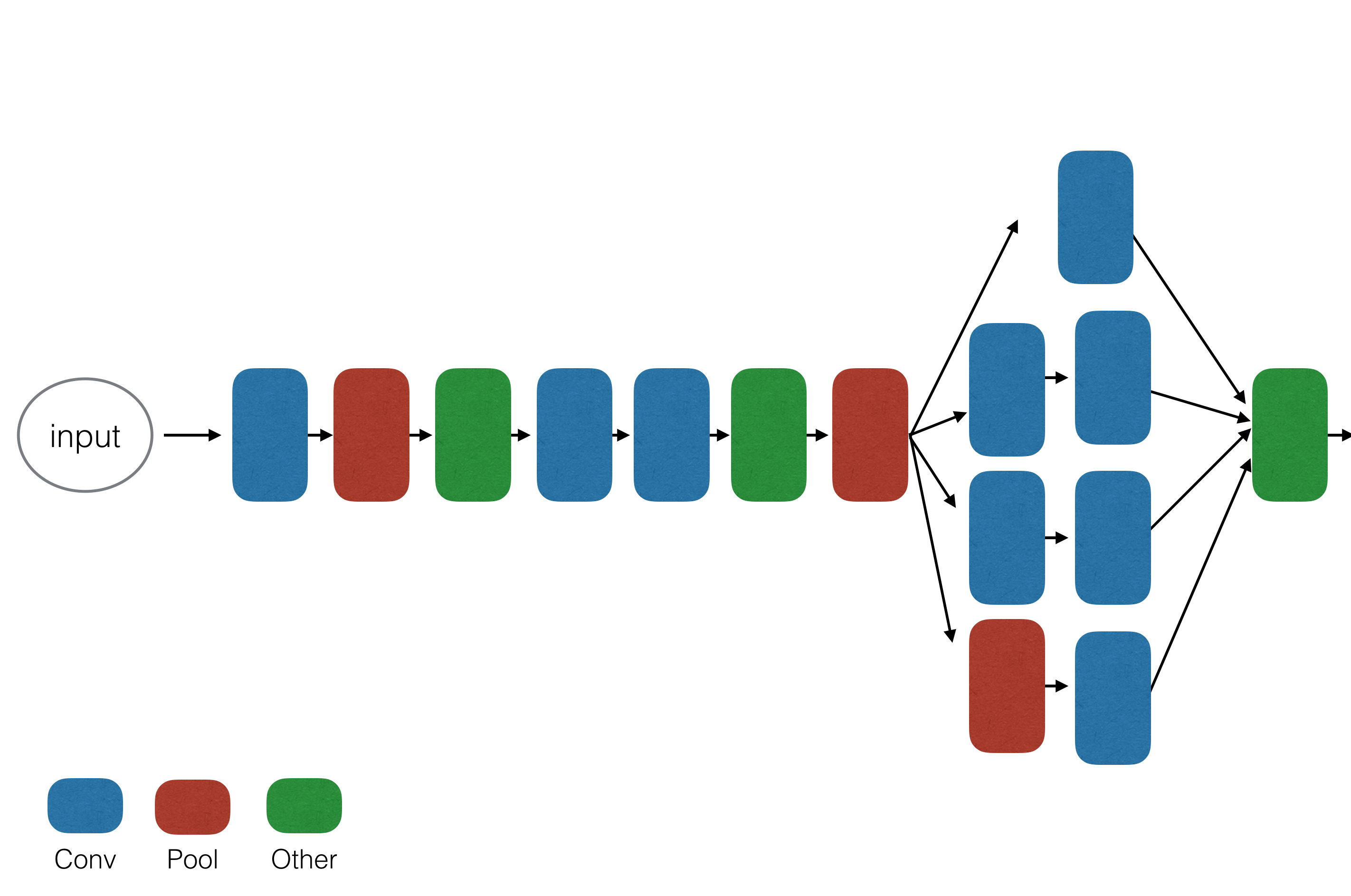
The novel idea GoogLeNet introduced was the Inception Module, which consists of parallel 1x1, 3x3 and 5x5 Conv filters with an additional pooling filter followed by a depthwise concatenation. The inception module is more efficient than single Conv layers, because it can capture combined features at a single scale. The inception module heavily uses 1x1 convolutions. These so-called Bottleneck Convolutions perform a weighted sum of the input volume along the depth dimension. This property is very handy to reduce the number of depth dimensions when concatenating convolutions, and to reduce correlations within the individual activations.
Another technique to drastically reduce model parameters is the backend, which consists of an average pooling operation instead of an expensive softmax classifier with fully connected layers. Therefore, the number of trainable parameters in GoogLeNet is less than seven million.
The biggest finding of GoogLeNet is the introduction of the inception module and the usage of bottleneck convolutions. More recent development at Google, such as the Xception model by Chollet or AutoML, discovered even more complicated inception-like wide modules to further improve the performance. A main take away from these wide modules is that it shows how you can improve the performance and accuracy of a network without piling convolutional layers sequentially.
ResNet
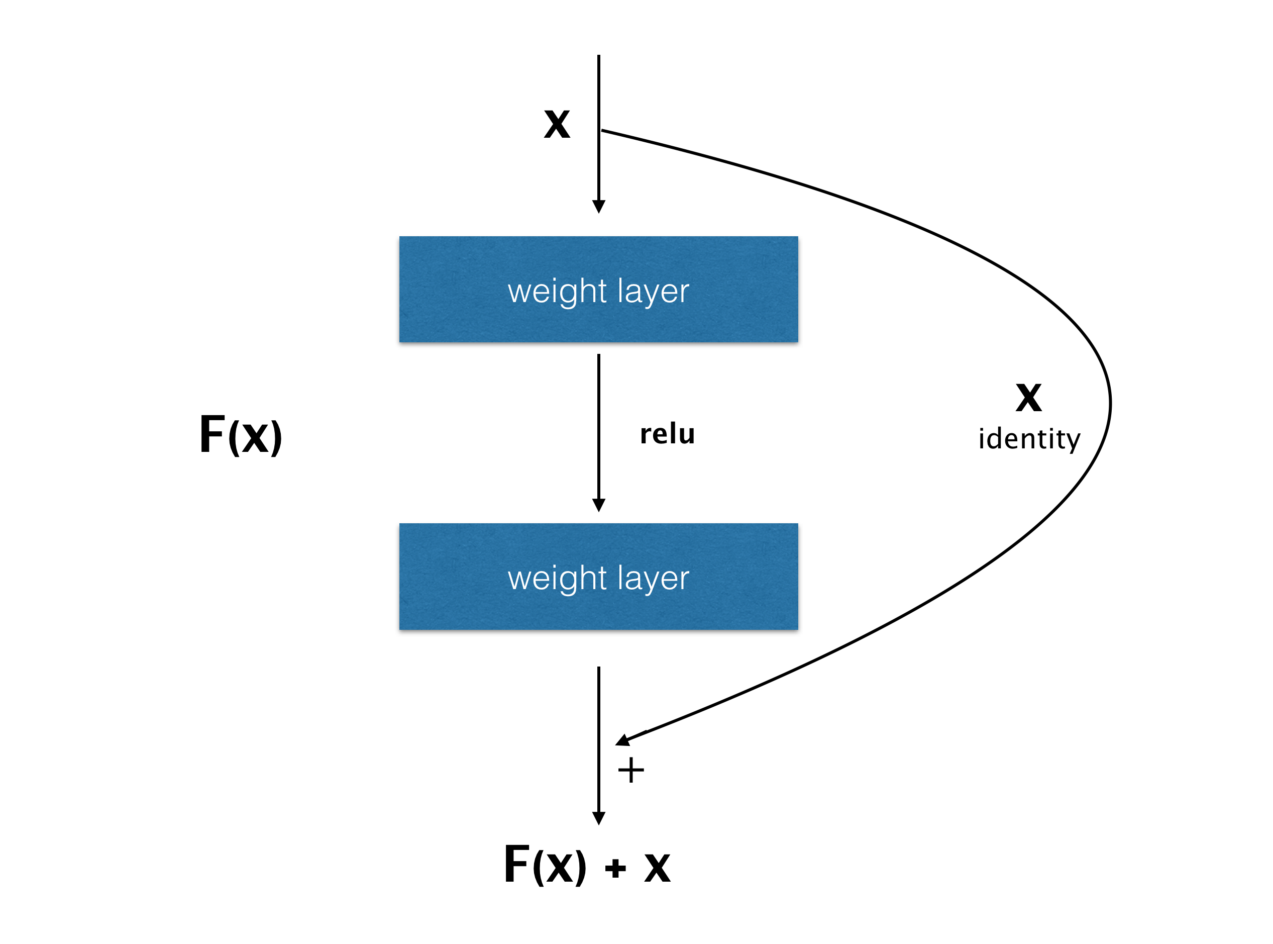
ResNet, or residual neural network, was introduced by Kaiming He at Microsoft. It achieved an incredible error rate of 3.6% in ILSVRC 2015, which is better than the human performance for image classification. What’s noteworthy about ResNet is the large amount of layers ResNet has. It has 152 layers in total, which is the largest network introduced in this section. The Skip Connection architecture of this network is also a notable idea. This is a technique to create new connections, and skipping some layers. This skipped block is called the Residual Block.
It is well known that simply deepening the layers causes degradation problems. While many layers are needed to improve the accuracy, too many layers make it worse. When stacking too many Conv layers, the gradient will diminish while backpropagating through the network, so training becomes impossible. The number of layers is a trade-off.
The core concept, or the residual block, to solve this challenge is simple. As shown in the previous figure, there is an identity connection to skip several convolutional layers. In this block, the network parameter is trained to predict the residual of the input from the target value. Instead of learning the target output, ResNet tries to learn the residual itself. Residual tends to be sensitive to the small change of the input. The same notion applies to the gradient. The residual connection also has the nice property that the gradient is passed into the residual block, as well as directly to the input of the residual block.
That’s why ResNet achieves the best performance with deeper layers while keeping fewer network parameters. Since there are many improved versions of ResNet, it may be the most promising architecture to use.
SqueezeNet
SqueezeNet is a small deep learning model designed to run on mobile, on embedded, or on an IoT device. The original paper’s title is “AlexNet-level accuracy with 50x fewer parameters and < 0.5MB model size.”
SqueezeNet is aimed to achieve a fewer number of parameters without losing the accuracy. The following table shows how much SqueezeNet can save memory space. Comparing with the compressed AlexNet model, SqueezeNet is far smaller than AlexNet without losing the accuracy performance.
| CNN Architecture | Compression Approach | Data Type | Original > Compressed | ImageNet Accuracy |
|---|---|---|---|---|
| AlexNet | None(baseline) | 32bit | 240MB | 80.3% |
| AlexNet | Deep Compression(Han et al.,2015a) | 5-8bit | 240MB > 6.9MB | 80.3% |
| SqueezeNet | None | 32bit | 4.8MB | 80.3% |
| SqueezeNet | Deep Compression | 8bit | 4.8MB→0.66MB | 80.3% |
| SqueezeNEt | Deep Compression | 6bit | 4.8MB→0.47MB | 80.3% |
There are mainly three interesting strategies SqueezeNet introduced.
- It uses 1x1 bottleneck convolutions instead of 3x3 filters, because the former has only 1/9 the number of parameters.
- It uses 1x1 bottleneck convolutions to reduce the number of input channels so that following later can reduce the computation.
- It uses downsampling to keep a big feature map to improve performance.
Strategies 1 and 2 are used for reducing the size of the model, and Strategy 3 is used for keeping the accuracy. The building block of SqueezeNet for that purpose is called the fire module, which is composed of squeeze layer and expand layer as shown in the next figure.

Squeeze layer reduces the number of input channels to following an expand layer. That corresponds to Strategy 2. The expand layer filters the input by using 1x1 layer and 3x3 layers. A 1x1 filter is used for reducing the number of parameters of the layer. It corresponds to Strategy 1. By using the fire module, it is possible to reduce the size of the SqueezeNet model. SqueezeNet has pooling layers that are used for down sampling. As shown in Strategy 3, these layers are put after convolutional layers. The following figure is an illustration of the whole architecture of SqueezeNet.

You can see a bunch of fire modules used in layers. Since SqueezeNet can achieve the same performance result as AlexNet, while keeping the size smaller, it is good to use the model on the client side like a mobile device or IoT device.
Recurrent neural network (RNN)
Since CNN is very good at extracting any kind of features from the image in a robust way, it is mainly used for the field of image recognition. But you should not use CNN to process a sequential data like time series data or natural language, because it is not efficient. A recurrent neural network is a model to solve such a problem. It keeps storing previous states to predict the following outputs based on past history. Let’s say we have to predict the last word of a sentence. Let’s assume we say, “I am learning deep learning.” It’s natural to think that the last word “learning” depends on the previous words, “I am learning deep.” In short, it is necessary to remember some previous words in order to let the deep neural network say something properly. U, W, and V are the weight matrix. x is an input vector. h is a hidden layer that is also used as an internal state of RNN. The following figure shows what RNN looks like.

RNN has hidden layers whose output will be the input in the following time. In the previous figure, h(t-1) at time t-1 will be the input of h(t) at time t. RNN receives one input from the sequential data and predicts one output. The output of the hidden layer is used as the internal state. It will be passed to the hidden layer as the input in next time. The internal state is calculated by all of the previous states so that RNN is able to consider the sequence of data in the past.
Although RNN was developed in the 1980s, it could not achieve high accuracy with the deep neural network. The training is often done by backpropagation through time (BPTT) which is similar to backpropagation of the normal feedforward deep neural network. The loop in RNN can be seen as the variable length chain of a network. You are able to find a normal neural network by unfolding the loop.
In that way, the gradient can vanish as the network becomes deeper, which indicates that the weights of the layers are hardly updated. It was difficult to train a deep RNN with reasonable accuracy because the dependencies between far inputs are not often considered.
LSTM and GRU are introduced to avoid gradient vanishing problems in RNN.
LSTM
Long-Short Term Memory (LSTM) was originally invented by Hochreiter and Schmidhuber in 1997. It applied to deep RNN architecture around 2007 and achieved a significant result in speech recognition. LSTM attached a new unit to RNN to learn long-term dependency. The unit is used to learn when to take the internal state in and out in a sequence. Instead of having a single neural network layer, LSTM is composed of four units: CEC, input gate, output gate, and forget gate.
CEC: It’s an acronym of “constant error carousel.” The unit keeps the value in the previous state as it is. CEC in the LSTM block just multiplies 1 to the input and returns the value in next time. This is the core component of LSTM. Thanks to CEC, the gradient of layers does not vanish even if the network becomes deeper.
Input gate and output gate: These units control when to fire the CEC unit. CEC passes all past values to next state even if there is no dependency between these times. That is a reason why these kind of gates are necessary. Input gate and output gate are opened only when needed. These gates are closed to keep the past data in other cases. The gates are also trainable as well as other layers to let itself open/close at an appropriate time.
Forget gate: By introducing CEC and input/output gates, it is possible to consider long-term dependency. On the other hand, there is a case when you don’t need the memory stored in the past because the data pattern is drastically changed. It is efficient to clear the value stored in LSTM in such cases. Forget gate is responsible for managing when to reset the value in CEC. Forget gate decides when to clear the value based on the input value and the past state.
The following figure shows what the LSTM block looks like. Red circles represent input gate, forget gate, and output gate respectively. They activate a neural with given input value. Dot line input represents a value passed from the past, which stores historic state.

These four units construct an LSTM block and properly manage the past history state. Please remember that LSTM is also a trainable block so that we don’t need to take care of how long LSTM should store the past history or when to clear it. It is all learned through an optimization process.
GRU
LSTM is a promising way to learn long-term dependency. But it has many parameters and the computation process is costly. If you can make use of a unit that achieves the same level performance with less computation cost, it must be better. GRU (Gated Recurrent Unit) was invented in 2014 by Kyunghyun Cho et al. It is a unit that can replace LSTM. GRU is composed of only two gates: reset gate and update gate.
As you can see in the following figure, GRU is simpler than the LSTM component.
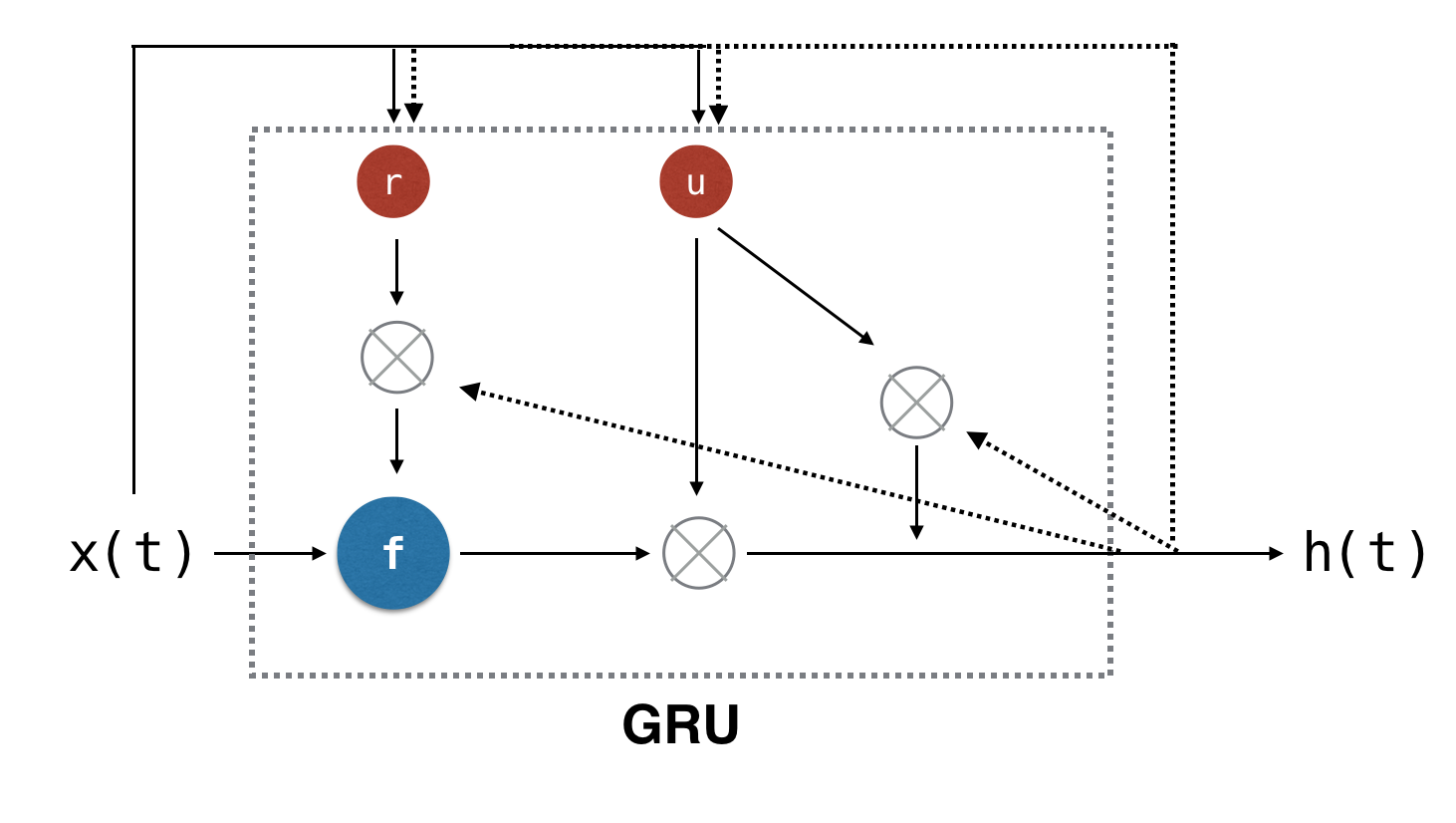
Both reset gate and update gate calculate their own output from the input value and the past state. The output of reset gate is used for deciding whether to use the previous state. The output of update gate is used as a weight to decide the ratio between past state and current state. GRU has fewer parameters than LSTM has. You can expect faster performance in both training and inference state.
Deep reinforcement learning
Both CNN and RNN are usually used in the context of supervised learning, which means you need to give some target values to the corresponding input. Reinforcement learning is another kind of field in machine learning. It is necessary to give a model reward on the situation. So a model (called agent in reinforcement learning) takes an action against an environment around it to make the total reward maximize as shown in the next figure.
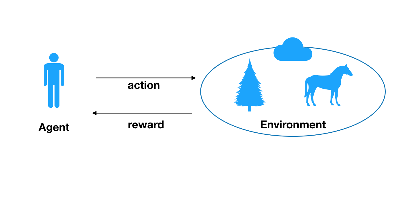
All agent can know are rewards given to each agent’s action and the situation around the agent. For example, there is an agent in a maze. The agent does not know how to reach the goal of the maze. A reward is given to the agent in every step. The reward becomes higher and higher in proportion as it reaches the goad. It is necessary for the agent to search the correct route to reach the goal by maximizing the total reward it receives. What is challenging is the agent cannot correctly know the reward it receives in the future because it depends on the action that agent takes. Theoretically, the problem can be formalized as a Markov Decision Process (MDP).
- A finite set of states: There are possible positions of the agent in the maze.
- A set of actions available in each step: Agent can go up/down/left/right if no wall exists.
- Transitions between states according to the agent action: If the agent goes up, walls around the agent and the distance to the goal are changed.
- A discount of reward factor between 0 and 1: It controls the importance of the reward in a time series. A reward obtained in the future tends to be less important than the reward now.
So the objective of the agent can be expressed like this.

A reward R depends on the action and state in time t. The reward is discounted by the factor gamma. So the agent is required to learn the way to maximize this total reward G. It is called a discounted total reward. The most famous algorithm to maximize the total reward is Q-learning.
Q-learning is an algorithm to learn which action to take based on the map function called action-value function, which is a function to return expected total reward with a given state and action. The agent should take an action that maximizes the estimated total reward returned by the function.
![]()
Formula2 represents an expected total reward with a given state and action. S is a state and A is an action in the time t respectively. This kind of total reward is often represented with capital Q. So it’s called Q-learning. That’s simple. But how can we get such magical function?
The function is initially not working properly. It always returns the same value or a random value. The function must be updated based on the actual reward the agent receives through exploration according to this formula.
![]()
In every step, the function is updated based on the formula. Alpha is a learning rate and gamma is a discount rate multiplied by rewards. We are not going to deep dive into the detail here, but it is known that Q-learning can find the optimal solution eventually with any finite MDP. By using the optimal function, the agent can find the optimal action for every possible state. The agent does not necessarily choose the optimal action every time. Randomly choosing a suboptimal action can make the search space wider so that the agent can have more time on exploitation.
There is another approach to do Q-learning instead of having an action-value function. As you may have noticed, we can have a function that predicts the next action from the current state directly, which is called policy learning. That is a straightforward way to infer that next action be taken instead of just calculating the expected total reward.
But what if the input state is too complex to infer the next action efficiently with simple mapping table? This is the time to use a deep neural network for reinforcement learning.
DQN
DQN (Deep Q Network) is a deep neural network used for Q-learning. It was invented by DeepMind in 2015 to beat human benchmarks across many Atari games, like Pong. DQN receives pixels of the input image (e.g. a frame of a game) and returns the estimated rewards for each action. Since a deep neural network is good at recognizing the characteristics of an image, DQN can find the necessary information to provide a good estimation of total rewards. But contributions of DQN is not limited to using a deep neural network for reinforcement learning. Deep neural network in reinforcement learning tends to be unstable in a learning process. There are two main findings to resolve the issue in DQN.
- Experience Replay: In order to avoid overfitting to specific state transitions, all state transitions experienced by the agent are stored. It is used to train DQN later in a mini-batch manner. It achieves not only improvement of accuracy but also learning speed by a mini-batch algorithm.
- Skipping Frames: The Atari game environment has 60 images per second. But humans don’t take that many actions in a second. So this technique let DQN calculate the estimation at every four frames. It reduces the computational cost significantly without losing the accuracy.
| B.Rider | Breakout | Pong | S.Invaders | |
|---|---|---|---|---|
| Random | 354 | 1.2 | -20.4 | 179 |
| DQN | 4092 | 168 | 20 | 581 |
| Human | 7456 | 31 | -3 | 3690 |
This table shows the average total reward for various learning algorithms when playing Atari games. It shows that DQN outperforms even humans in some games. Basically, DQN obtained human-level control on some Atari games. The most famous application of deep reinforcement learning is AlphaGo. AlphaGo defeated several chess players in the world. That was the memorial event that impressed us how machines can think complicated concepts like a human.
Summary
In this chapter, we introduced several state of the art deep learning models. Each model is designed to solve a problem in a specific field. CNN can be used for image processing such as object detection. This model is good at extracting useful feature from raw image data. You can use RNN to process time-series data, including natural language processing. This model is already used by famous machine translation systems like Google Translate. Last but not least, deep reinforcement learning models show remarkable results by beating human performance, especially in the field of games. The result of deep reinforcement learning reminds us of the arrival of artificial intelligence. Be sure to keep an eye on the new deep learning architectures.