There are many aspects in nature that are repeating and many cases of patterns similar at different scales. For example, when observing a pine tree, one may notice that the shape of a branch is very similar to that of the entire tree, and the shapes of sub-branches and the main branch are also similar. Such kind of self-similar structure that occurs at different levels of magnification can be modeled by a branch of mathematics called Fractal geometry. The term fractal was coined by Benoît Mandelbrot in 1975, and means fractus or broken in Latin. Fractal geometry studies the properties and behavior of fractals. It describes many situations which cannot be explained easily by classical geometry. Fractals can be used to model plants, weather, fluid flow, geologic activity, planetary orbits, human body rhythms, socioeconomic patterns, and music, just to name a few. They have been applied in science, technology, and computer generated art. For example, engineers use fractals to control fluid dynamics in order to reduce process size and energy use.
A fractal, typically expressed as curves, can be generated by a computer recursively or iteratively with a repeating pattern. Compared with human beings, computers are much better in processing long and repetitive information without complaint. Fractals are therefore particularly suitable for computer processing. This chapter introduces the basic concepts and program implementation of fractals. It starts with a simple type of fractal curves, then focuses on a grammar-based generic approach for generating different types of fractal images, and finally discusses the well-known Mandelbrot set.
A simple example of self-similar curves is the Koch curve, discovered by the Swedish mathematician Helge von Koch in 1904. It serves a useful introduction to the concepts of fractal curves.
In Figure 8.1, K0, K1, and K2 denote successive generations of the Koch curve. A straight line segment is called the zero-th generation. We can construct Koch curve as follows:
Begin with a straight line and call it K0;
Divide each segment of Kn into three equal parts; and
Replace the middle part by the two sides of an equilateral triangle of the same length as the part being removed.
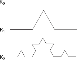
The last step ensures that every straight line segment of Kn becomes the shape of K1 in a smaller scale in Kn+1.
Koch curves have the following interesting characteristics:
Each segment is increased in length by a factor of 4/3. Therefore, Kn+1 is 4/3 as long as Kn, and Ki has the total length of (4/3)i.
When n is getting large, the curve still appears to have the same shape and roughness.
When n becomes infinite, the curve has an infinite length, while occupying a finite region in the plane.
The Koch curve can be easily implemented using the turtle graphics method. Originated in the Logo programming language, turtle graphics is a means of computer drawing using the concept of a turtle crawling over the drawing space with a pen attached to its underside. The drawing is always relative to the current position and direction of the turtle. Considering each straight line of Kn−1 to be drawn as a K1 in Kn in the next generation, we can write a recursive program to draw Koch curves as in the following pseudocode:
To draw Kn we proceed as follows:
If  (n == 0) Draw a straight line;
Else
{  Draw Kn-1;
   Turn left by 60°;
   Draw Kn-1;
   Turn right by 120°;
   Draw Kn-1;
   Turn left by 60°;
   Draw Kn-1;
}
To implement the above pseudocode in a Java program, we need to keep track of the turtle's current position and direction. The following program draws the Koch curve at the zero-th generation K0. With each mouse click, it draws a higher generation replacing the previous generation. The program defines the origin of the coordinate system at the center of the screen. The turtle starts pointing to the right, and locating at half of the initial length to the left of the origin, that is, (−200, 0) for the initial length of 400. The turtle moves from the current position at (x, y) to the next position at (x1, y1) while changing its direction accordingly.
// Koch.java: Koch curves.
import java.awt.*;
import java.awt.event.*;
public class Koch extends Frame
{  public static void main(String[] args){new Koch();}
   Koch()
   {  super("Koch. Click the mouse button to increase the level");
      addWindowListener(new WindowAdapter()
         {public void windowClosing(
                 WindowEvent e){System.exit(0);}});
      setSize (600, 500);
      add("Center", new CvKoch());
show();
}
}
class CvKoch extends Canvas
{ public float x, y;
double dir;
int midX, midY, level = 1;
int iX(float x){return Math.round(midX+x);}
int iY(float y){return Math.round(midY-y);}
CvKoch()
{ addMouseListener(new MouseAdapter()
{ public void mousePressed(MouseEvent evt)
{ level++; // each mouse click increases the level
repaint();
}
});
}
public void paint(Graphics g)
{ Dimension d = getSize();
int maxX = d.width - 1, maxY = d.height - 1,
length = 3 * maxX / 4;
midX = maxX/2; midY = maxY/2;
x = (float)(-length/2); // Start point
y = 0;
dir = 0;
drawKoch(g, length, level);
}
public void drawKoch(Graphics g, double len, int n)
{ if (n == 0)
{ double dirRad, xInc, yInc;
dirRad = dir * Math.PI/180;
xInc = len * Math.cos(dirRad); // x increment
yInc = len * Math.sin(dirRad); // y increment
float x1 = x + (float)xInc,
y1 = y + (float)yInc;
g.drawLine(iX(x), iY(y), iX(x1), iY(y1));
x = x1;
y = y1;}
else
{ drawKoch(g, len/=3, --n);
dir += 60;
drawKoch(g, len, n);
dir-=120;
drawKoch(g, len, n);
dir += 60;
drawKoch(g, len, n);
}
}
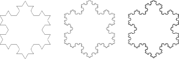
}Joining three Koch curves together, we obtain the interesting Koch snowflake as shown in Figure 8.2. The length of a Koch snowflake is 3*(4/3)i for the ith generation since the length of Ki is (4/3)i. It increases infinitely as does i. The area of the Koch snowflake grows slowly and is indeed bounded. In fact, as i becomes very large, its shape and roughness appear to remain the same. Koch snowflakes can be easily drawn by connecting three Koch curves using a modified version of the program above (see Exercise 8.2).
As discussed above, Koch curves are drawn through a set of commands specifically defined for Koch curves. Many interesting curves could be drawn in a similar fashion but they would require a complete program for each different kind of curve. The approach in the above section is apparently not general for generating different kinds of curves.
Consider again the Koch curve. The pattern of the first generation repeats itself in smaller scales at higher generations.
Such a common pattern distinguishes Koch curves from other curves. Therefore, an approach that can encode the common pattern in a simple string of characters would be general enough to specify a variety of curves. Formally, the specification of a common pattern is called a grammar, and the grammar-based systems for drawing fractal curves are called L-Systems (invented by the Hungarian biologist Aristid Lindenmayer in 1968).
The string of characters defining a common pattern instructs the turtle to draw the pattern. Each character in the string serves as a command to perform an atomic operation. Given the distance D and turning angle α through which the turtle is supposed to move, let us now introduce the three most common commands:
F - move forward the distance D while drawing in the current direction.
+ - turn right through the angle α.
− - turn left through the angle α.
For example, given a string F−F++F−F and angle 60°, the turtle would draw the first generation of Koch curve K1 as shown in Figure 8.1. It would however be tedious and error-prone to manually provide long strings for different curves. Fortunately, computers are best at performing repeated, long and tedious tasks without making mistakes. Using the same Koch curve example, to draw more generations, we define a string production rule
| F → F−F++F−F |
The rule means that every occurrence of F (that is, the left-hand side of '→') should be replaced by F−F++F−F (that is, the right-hand side). Starting from an initial string F which is called the axiom, recursively applying this production rule would produce strings of increasing lengths. Interpreting any of the strings, the turtle would draw a corresponding generation of the Koch curve. Let us make the axiom the zero-th generation K0 = F and the first generation K1 = F−F++F−F, then K2 can be obtained by substituting every F character in K1 by F−F++F−F, so that
| K2 = F−F++F−F−F−F++F−F++F−F++F−F−F−F++F−F |
By interpreting this string, the turtle would draw a curve exactly the same as K2 in Figure 8.1. This process can continue to generate the Koch curve at any higher generation.
In summary, to draw a fractal curve, such as the Koch curve, at any generation, we need to know at least the following three parameters:
The axiom from which the turtle starts.
The production rule for producing strings from the F character. We will call the right-hand side of this rule the F-string, which is sufficient to represent the rule.
The angle at which the turtle should turn.
Denoting these parameters in a template form (axiom, F-string, angle), we call this the grammar of the curve, and we can specify the Koch curve as (F, F−F++F−F, 60).
To define more complex and interesting curves, we introduce three more production rules, obtaining grammars of six elements instead of three as above. We introduce an X-string, to be used to replace every occurrence of X when producing the next generation string. Similarly, there will be a Y-string, used to replace every occurrence of Y. Their replacement process is performed in the same fashion as for the F-string. In other words, all the three string types are treated equally during the string-production process. The X and Y characters are, however, different from the F character as they are simply ignored by the turtle when drawing the curve. The third new production rule, named f-string, will be discussed shortly. In the meantime, we reserve its position, but substitute nil for it to indicate that we do not use it. It follows that there are six parameters in the extended grammar template
| (axiom, F-string, f-string, X-string, Y-string, angle). |
The following grammars produce some more interesting curves:
| Dragon curve: (X, F, nil,X+YF+,−FX−Y, 90). |
| Hilbert curve: (X, F, nil−YF+XFX+FY−,+XF−YFY−FX+, 90). |
| Sierpinski: arrowhead(YF, F, nil, YF+XF+Y, XF−YF−X, 60). |
Figures 8.3, 8.4 and 8.5 illustrate some selected generations of the Dragon, Hilbert and Sierpinski curves that are generated based on their string grammars as defined above.

It is remarkable that no Dragon curve intersects itself. There seems to be one such intersection in the 4th generation Dragon curve of Figure 8.3 and many more in those of higher generations. However, that is not really the case, as demonstrated by using rounded instead of sharp corners. Figure 8.4 illustrates this for an 8th generation Dragon curve.
It is interesting to note that all the curves we have seen so far share one common characteristic, that is, each curve reflects the exact trace of the turtle's movement and is drawn essentially as one long and curved line. This is because the turtle always moves forward and draws by executing the F character command.


Sometimes, it is desirable to keep some of the curve components at proper distances from each other. This implies that such a curve is not connected. We therefore need to define a forward moving action for the turtle without drawing:
f - move forward the distance D without drawing a line.
The f-string, for which we have already reserved a position (just after the F-string) indicates how each lower-case f is to be expanded. By using an f-string other than nil, we are able to generate an image with a combination of islands and lakes as shown in Figure 8.6, based on the following grammar:
| (F+F+F+F, F+f−FF+F+FF+Ff+FF−f+FF−F−FF−Ff−FFF, ffffff, nil, nil, 90) |
Note that here the parameters X-string and Y-string are unused and therefore written as nil.

To summarize, we have introduced the following six parameters into our string grammar:
The axiom from which the turtle starts;
The F-string for producing strings from F that instructs the turtle to move forward while drawing;
The f-string for producing strings from f, that instructs the turtle to move forward without drawing;
The X-string for producing strings from X, that does not affect the turtle;
The Y-string for producing strings from Y, that does not affect the turtle; and
The angle at which the turtle should turn.
In principle, more parameters may be introduced if the above six parameters cannot express new types of curves. On the other hand, a grammar does not have to use all the introduced parameters since, as we have seen, a nil can be used to represent an unused parameter.
With all the curves we have seen so far, one may observe the following phenomenon. The turtle is always moving forward along a curved line. It sometimes draws (seeing an F character) and sometimes does not draw (seeing an f character). The turtle never turns back to where it has visited before, since it cannot remember its previous positions. This implies that the turtle is unable to branch off from any of the previous curve positions and draw branching lines.
To make the turtle remember places that it has visited, we need to introduce the concept of the turtle's state. Let us call the turtle's current position together with its direction the state of the turtle. In other words, a state is defined by the values of a location in the drawing space and the angle at the location. To enhance the drawing power of string-production rules, we allow the turtle to keep its states and return to any of them later by introducing two more character commands:
[- store the current state of the turtle
] - restore the turtle's previously stored state
These two characters, however, do not form strings of their own and thus do not require new production rules. They merely participate in the F-, f-, X-, and Y-strings to instruct how the turtle should behave.
The most appropriate data structure to implement the store and restore operations is a stack. Upon meeting a [ character, the turtle pushes its current state onto the stack. When encountering a ] character, the turtle pops its previous state from the stack and starts from the previous position and direction to continues its journey. Having empowered the turtle with the capability of returning and restarting from its previous states, we are able to draw curves with branches, such as trees defined in the following string grammars:
| Tree1: (F, F[+F]F[−F]F, nil, nil, nil, 25.7) |
| Tree2: (X, FF, nil, F[+X]F[−X]+X, nil, 20.0) |
| Tree3: (F, FF−[−F+F+F]+[+F−F−F], nil, nil, nil, 22.5) |
These grammars were used to obtain the trees shown in Figure 8.7.
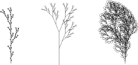
Figure 8.7. Examples of fractal trees: Tree1 (4th generation), Tree2 (5th generation) and Tree3 (4th generation)
If the line thickness of each branch is set in proportion to its distance from the root, and also a small fraction of randomness is applied to the turning angle, more realistic looking trees would be produced.
Most of the figures in this section were produced by the program below, with input files to be discussed after this program:
// FractalGrammars.java
import java.awt.*;
import java.awt.event.*;

public class FractalGrammars extends Frame
{  public static void main(String[] args)
   {  if (args.length == 0)
         System.out.println("Use filename as program argument.");
      else
         new FractalGrammars(args[0]);
   }
   FractalGrammars(String fileName)
   {  super("Click left or right mouse button to change the level");
      addWindowListener(new WindowAdapter()
         {public void windowClosing(
                 WindowEvent e){System.exit(0);}});
      setSize (800, 600);
      add("Center", new CvFractalGrammars(fileName));
      show();
  }
}

class CvFractalGrammars extends Canvas
{  String fileName, axiom, strF, strf, strX, strY;
   int maxX, maxY, level = 1;
   double xLast, yLast, dir, rotation, dirStart, fxStart, fyStart,
      lengthFract, reductFact;

   void error(String str)
   {  System.out.println(str);
      System.exit(1);
   }

   CvFractalGrammars(String fileName)
   {  Input inp = new Input(fileName);
      if (inp.fails())
         error("Cannot open input file.");
axiom = inp.readString(); inp.skipRest();
strF = inp.readString(); inp.skipRest();
strf = inp.readString(); inp.skipRest();
strX = inp.readString(); inp.skipRest();
strY = inp.readString(); inp.skipRest();
rotation = inp.readFloat(); inp.skipRest();
dirStart = inp.readFloat(); inp.skipRest();
fxStart = inp.readFloat(); inp.skipRest();
fyStart = inp.readFloat(); inp.skipRest();
lengthFract = inp.readFloat(); inp.skipRest();
reductFact = inp.readFloat();
if (inp.fails())
error("Input file incorrect.");
addMouseListener(new MouseAdapter()
{ public void mousePressed(MouseEvent evt)
{ if ((evt.getModifiers() & InputEvent.BUTTON3_MASK) != 0)
{ level--; // Right mouse button decreases level
if (level < 1)
level = 1;
}
else
level++; // Left mouse button increases level
repaint();
}
});
}
Graphics g;
int iX(double x){return (int)Math.round(x);}
int iY(double y){return (int)Math.round(maxY-y);}
void drawTo(Graphics g, double x, double y)
{ g.drawLine(iX(xLast), iY(yLast), iX(x) ,iY(y));
xLast = x;
yLast = y;
}
void moveTo(Graphics g, double x, double y)
{ xLast = x;
yLast = y;
}public void paint(Graphics g)
{ Dimension d = getSize();
maxX = d.width - 1;
maxY = d.height - 1;
xLast = fxStart * maxX;
yLast = fyStart * maxY;
dir = dirStart; // Initial direction in degrees
turtleGraphics(g, axiom, level, lengthFract * maxY);
}
public void turtleGraphics(Graphics g, String instruction,
int depth, double len)
{ double xMark=0, yMark=0, dirMark=0;
for (int i=0;i<instruction.length();i++)
{ char ch = instruction.charAt(i);
switch(ch)
{
case 'F': // Step forward and draw
// Start: (xLast, yLast), direction: dir, steplength: len
if (depth == 0)
{ double rad = Math.PI/180 * dir, // Degrees -> radians
dx = len * Math.cos(rad), dy = len * Math.sin(rad);
drawTo(g, xLast + dx, yLast + dy);
}
else
turtleGraphics(g, strF, depth - 1, reductFact * len);
break;
case 'f': // Step forward without drawing
// Start: (xLast, yLast), direction: dir, steplength: len
if (depth == 0)
{ double rad = Math.PI/180 * dir, // Degrees -> radians
dx = len * Math.cos(rad), dy = len * Math.sin(rad);
moveTo(g, xLast + dx, yLast + dy);
}
else
turtleGraphics(g, strf, depth - 1, reductFact * len);
break;
case 'X':
if (depth > 0)
turtleGraphics(g, strX, depth - 1, reductFact * len);
break;
case 'Y':
if (depth > 0)turtleGraphics(g, strY, depth - 1, reductFact * len);
break;
case '+': // Turn right
dir -= rotation; break;
case '-': // Turn left
dir += rotation; break;
case '[': // Save position and direction
xMark = xLast; yMark = yLast; dirMark = dir; break;
case ']': // Back to saved position and direction
xLast = xMark; yLast = yMark; dir = dirMark; break;
}
}
}
}The most essential input data consist of the grammar, for example,
| (X, F, nil, X+YF+, −FX−Y, 90) |
for the Dragon curve. In addition, the following five values would help in obtaining desirable results:
The direction in which the turtle starts, specified as the angle, in degrees, relative to the positive x-axis.
The distance between the left window boundary and the start point, expressed as a fraction of the window width.
The distance between the lower window boundary and the start point, expressed as a fraction of the window height.
The length of a single line segment in the first generation, expressed as a fraction of the window height.
A factor to reduce the length in each next generation, to prevent the image from growing outside the window boundaries.
Setting the last two values can be regarded as tuning, so they were found experimentally. We supply all these data, that is, five strings and six real numbers, in a file, the name of which is supplied as a program argument. For example, to produce the Dragon curve, we can enter this command to start the program:
java FractalGrammars Dragon.txt
where the file Dragon.txt is listed below, showing the grammar (X, F, X+YF+, −FX−Y, 90) followed by the five values just discussed:
"X"      // Axiom
"F"      // strF
""       // strf
"X+YF+"  // strX
"-FX-Y"  // strY
90       // Angle of rotation
0        // Initial direction of turtle (east)
0.5      // Start at x = 0.5 * width
0.5      // Start at y = 0.5 * height
0.6      // Initial line length is 0.6 * height
0.6      // Reduction factor for next generation
As you can see, strings are supplied between a pair of quotation marks, and comment is allowed at the end of each line. Instead of nil, we write the empty string "". Although the initial direction of the turtle is specified as east, the first line is drawn in the direction south. This is because of the axiom "X", which causes initially strX = "X+YF+" to be used, where X and Y are ignored. So actually "+F+" is executed by the turtle. As we know, the initial + causes the turtle to turn right before the first line is drawn due to F, so this line is drawn downward instead of from left to right.
The other curves were produced in a similar way. Both the grammars and the five additional parameter values, as discussed above, for these curves are listed in the following table:
Dragon | (X, F, nil, X+YF+, −FX−Y, 90) | 0 | 0.5 | 0.5 | 0.6 | 0.6 |
Hilbert | (X, F, nil, −YF+XFX+FY−, +XF−YFY−FX+, 90) | 0 | 0.25 | 0.25 | 0.8 | 0.47 |
Sier-pinski | (YF, F, nil, YF+XF+Y, XF−YF−X, 60). | 0 | 0.33 | 0.5 | 0.38 | 0.51 |
Islands | (F+F+F+F, F+F−FF+F+FF+Ff+FF−f+FF−F−FF−Ff−FFF, ffffff, nil, nil, 90) | 0 | 0.25 | 0.65 | 0.2 | 0.2 |
Tree1 | (F, F[+F]F[−F]F, nil, nil, nil, 25.7) | 90 | 0.5 | 0.05 | 0.7 | 0.34 |
Tree2 | (X, FF, nil, F[+X]F[−X]+X, nil, 20.0) | 90 | 0.5 | 0.05 | 0.45 | 0.5 |
Tree3 | (F, FF−[−F+F+F]+[+F−F−F], nil, nil, nil, 22.5) | 90 | 0.5 | 0.05 | 0.25 | 0.5 |
When discussing the Tree examples with branches, we suggested that a stack would be used to push and pop states, while there seemed to be no stack structure in the program. However, there is a local variable xMark in the recursive method turtleGraphics, and for each recursive call a version of this variable is stored on a system stack. In other words, the use of a stack is implicit in this program.
The Mandelbrot set, named after Polish-born French mathematician Benoît Mandelbrot, is a fractal. Recall that a fractal curve reveals small-scale details similar to the large-scale characteristics. Although the Mandelbrot set is self-similar at different scales, the small-scale details are not identical to the whole. Also, the Mandelbrot set is infinitely complex. Yet the process of generating it is based on an extremely simple equation involving complex numbers. The left part of Figure 8.8 shows a view of the Mandelbrot set. The outline is a fractal curve that can be zoomed in for ever on any part for a close-up view, as the right part of Figure 8.8 illustrates. Even parts of the image that appear quite smooth show a jagged outline consisting of many tiny copies of the Mandelbrot set. For example, as displayed in Figure 8.8, there is a large black region like a cardioid near the center with a circle joining its left-hand side. The region where the cardioid and the circle are joined together appears smooth. When the region is magnified, however, the detailed structure becomes apparent and shows many fascinating details that were not visible in the original picture. In theory, the zooming can be repeated for ever, since the border is 'infinitely complex'.

The Mandelbrot set is a set M of complex numbers defined in the following way:
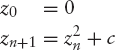
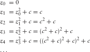
where C is the set of all complex numbers and, for some constant c, the sequence z0, z1, ... is defined as follows:
That is, the Mandelbrot set is the set of all complex numbers which fulfill the condition described above. In other words, if the sequence z0, z1, z2, . . . does not approach infinity, then c belongs to the set. Given a value c, the system generates a sequence of values called the orbit of the start value 0:
As soon as an element of the sequence {zn} is at a distance greater than 2 from the origin, it is certain that the sequence tends to infinity. A proof of this goes beyond the scope of this book. If the sequence does not approach infinity and therefore remains at a distance of at most 2 from the origin for ever, then the point c is in the Mandelbrot set. If any zn is farther than 2 from the origin, then the point c is not in the set.
Now let us consider how to generate a Mandelbrot image. Since the Mandelbrot set is a set of complex numbers, first we have to find these numbers that are part of the set. To do this we need a test that will determine if a given number is inside the set or outside. The test is applied to complex numbers zn computed as zn + 1 = zn2 + c. The constant c does not change during the testing process. As the number being tested, c is the point on the complex plane that will be plotted when the testing is complete. This plotting will be done in a color that depends on the test result. For some value nMax, say 30, we start computing z1, z2, . . . until either we have computed zn for n = nMax, or we have found a point zn (n ≤ nMax) whose distance from the origin O is greater than 2. In the former case, having computed nMax elements of the sequence, none of which is farther than a distance 2 away from O, we give up, consider the point c belonging to the Mandelbrot set, and plot it in black. In the latter case, the point zn going beyond the distance 2, we plot the point c in a color that depends on the value of n.
Let us now briefly discuss complex arithmetic, as far as we need it here, for those who are unfamiliar with this subject. Complex numbers are two-dimensional by nature. We may regard the complex number
| z = x + yi |
as the real number pair (x, y). It is customary to refer to x as the real part and to y as the imaginary part of z. We display z in the usual way, with x drawn along the horizontal axis and y along the vertical axis. Addition of two complex numbers is the same as that for vectors:
| (x1 + y1i) + (x2 + y2i) = (x1 + x2) + (y1 + y2)i |
By contrast, multiplication of complex numbers is rather complicated:
| (x1 + y1i)(x2 + y2i) = (x1x2 − y1y2) + (x1y2 + x2y1)i |
It follows that for
| z = x + yi |
we have
| z2 = (x2 − y2) + 2xyi |
Although we do not need this for our purpose, we may as well note that by setting x = 0 and y = 1, giving 0 + 1 × i = i, we find
| i2 = (02 − 12) + 2 × 0 × 1 × i = −1 |
which explains why the symbol i is often referred to as the square root of − 1:
The distance of the complex number z = x + yi from the origin O is called the absolute value or modulus of z and is denoted as |z|. It follows that
Remember, |z|2 = x2 + y2, while z2 = (x2 − y2) + 2xyi so, in general, |z|2 is unequal to z2. This very brief introduction to complex numbers cannot replace a thorough treatment as found in mathematics textbooks, but it will be sufficient for our Mandelbrot subject.
In the algorithm for Mandelbrot fractals, when computing each successive value of z, we want to know if its distance from the origin exceeds 2. To calculate this distance, usually denoted as |z|, we add the square of its distance from the x-axis (the horizontal real axis) to the square of its distance from the y-axis (the vertical imaginary axis) and then take the square root of the result. The computation of the square root operation can be saved by just checking whether the sum of these squares is greater than 4. In other words, for
| z = x + yi |
we perform the test
|z|2 > 4
which is expressed in terms of real numbers as
| x2 + y2 > 4 |
Now to compute each new value of z using zn + 1 = zn2 + c, let us write Re(c) and Im(c) for the real and imaginary parts of c. It then follows from
| z2 = (x + yi)2 = (x2 − y2) + (2xy)i |
that the real and imaginary parts of each element zn + 1 are found as follows:
| real part: xn + 1 = xn2 − yn2 + Re(c) |
imaginary part: yn + 1 = 2xnyn + Im(c)
As we increment n, the value of |zn|2 will either stay equal to or below 4 for ever, or eventually surpass 4. Once |zn|2 surpasses 4, it will increase for ever. In the former case, where the |zn|2 stays small, the number c being tested is part of the Mandelbrot set. In the latter case, when |zn|2 eventually surpasses 4, the number c is not part of the Mandelbrot set.
To display the whole Mandelbrot set image properly, we need some mapping
| xPix → x |
| yPix → y |
to convert the device coordinates (xPix, yPix) to the real and imaginary parts x and y of the complex number c = x + yi. In the program, the variables xPix and yPix are of type int, while x and y are of type double. We will use the following ranges for the device coordinates:
| 0 ≤ xPix < w |
| 0 ≤ yPix < h |
where we obtain the width w and height h of the drawing rectangle in the usual way:
w = getSize().width;
h = getSize().height;
For x and y we have
| minRe ≤ x ≤ maxRe |
| minIm ≤ y ≤ maxIm |
The user will be able to change these boundary variables minRe, maxRe, minIm and maxIm by dragging the left mouse button. Their default values are minRe0 = −2, maxRe0 = +1, minIm0 = −1, maxIm0 = +1, which will at any time be restored when the user clicks the right mouse button. Using the variable factor, computed in Java as
factor = Math.max((maxRe - minRe)/w, (maxIm - minIm)/h);
we can perform the above mapping from (xPix, yPix) to (x, y) by computing
| x = minRe + factor × xPix |
| y = minIm + factor × yPix |
For every device coordinate pair (xPix, yPix) of the window, the associated point c = x + iy in the complex plane is computed in this way. Then, in up to nMax iterations, we determine whether this point belongs to the Mandelbrot set. If it does, we display the original pixel (xPix, yPix) in black; otherwise, we plot this pixel in a shade of red that depends on n, the number of iterations required to decide that the point is outside the Mandelbrot set. The expression 100 + 155 * n/nMax ensures that this color value will not exceed its maximum value 255. If nMax is set larger than that in the program, program execution will take more time but the quality of the image would improve. The implementation of this can by found in the paint method at the bottom of the following program, after which we will discuss the implementation of cropping and zooming.
// MandelbrotZoom.java: Mandelbrot set, cropping and zooming in.
import java.awt.*;
import java.awt.event.*;

public class MandelbrotZoom extends Frame
{  public static void main(String[] args){new MandelbrotZoom();}
   MandelbrotZoom()
   {  super("Drag left mouse button to crop and zoom. " +
            "Click right mouse button to restore.");
      addWindowListener(new WindowAdapter()
         {public void windowClosing(
                 WindowEvent e){System.exit(0);}});
      setSize (800, 600);
      add("Center", new CvMandelbrotZoom());
      show();
   }
}
class CvMandelbrotZoom extends Canvas
{  final double minRe0 = −2.0, maxRe0 = 1.0,
                minIm0 = −1.0, maxIm0 = 1.0;
   double minRe = minRe0, maxRe =  maxRe0,
                  minIm = minIm0, maxIm =  maxIm0, factor, r;
   int n, xs, ys, xe, ye, w, h;

   void drawWhiteRectangle(Graphics g)
   {  g.drawRect(Math.min(xs, xe), Math.min(ys, ye),
Math.abs(xe - xs), Math.abs(ye - ys));
}
boolean isLeftMouseButton(MouseEvent e)
{ return (e.getModifiers() & InputEvent.BUTTON3_MASK) == 0;
}
CvMandelbrotZoom()
{ addMouseListener(new MouseAdapter()
{ public void mousePressed(MouseEvent e)
{ if (isLeftMouseButton(e))
{ xs = xe = e.getX(); // Left button
ys = ye = e.getY();
}
else
{ minRe = minRe0; // Right button
maxRe = maxRe0;
minIm = minIm0;
maxIm = maxIm0;
repaint();
}
}
public void mouseReleased(MouseEvent e)
{ if (isLeftMouseButton(e))
{ xe = e.getX(); // Left mouse button released
ye = e.getY(); // Test if points are really distinct:
if (xe != xs && ye != ys)
{ int xS = Math.min(xs, xe), xE = Math.max(xs, xe),
yS = Math.min(ys, ye), yE = Math.max(ys, ye),
w1 = xE - xS, h1 = yE - yS, a = w1 * h1,
h2 = (int)Math.sqrt(a/r), w2 = (int)(r * h2),
dx = (w2 - w1)/2, dy = (h2 - h1)/2;
xS -= dx; xE += dx;
yS -= dy; yE += dy; // aspect ration corrected
maxRe = minRe + factor * xE;
maxIm = minIm + factor * yE;
minRe += factor * xS;
minIm += factor * yS;
repaint();
}
}
}});
addMouseMotionListener(new MouseMotionAdapter()
{ public void mouseDragged(MouseEvent e)
{ if (isLeftMouseButton(e))
{ Graphics g = getGraphics();
g.setXORMode(Color.black);
g.setColor(Color.white);
if (xe != xs || ye != ys)
drawWhiteRectangle(g); // Remove old rectangle:
xe = e.getX();
ye = e.getY();
drawWhiteRectangle(g); // Draw new rectangle:
}
}
});
}
public void paint(Graphics g)
{ w = getSize().width;
h = getSize().height;
r = w/h; // Aspect ratio, used in mouseReleased
factor = Math.max((maxRe - minRe)/w, (maxIm - minIm)/h);
for(int yPix=0; yPix<h; ++yPix)
{ double cIm = minIm + yPix * factor;
for(int xPix=0; xPix<w; ++xPix)
{ double cRe = minRe + xPix * factor, x = cRe, y = cIm;
int nMax = 100, n;
for (n=0; n<nMax; ++n)
{ double x2 = x * x, y2 = y * y;
if (x2 + y2 > 4)
break; // Outside
y = 2 * x * y + cIm;
x = x2 - y2 + cRe;
}
g.setColor(n == nMax ? Color.black // Inside
: new Color(100 + 155 * n / nMax, 0, 0)); // Outside
g.drawLine(xPix, yPix, xPix, yPix);
}
}
}
}As indicated in the title bar (implemented by a call to super at the beginning of the MandelbrotZoom constructor), the user can zoom in by using the left mouse button. By dragging the mouse with the left button pressed down, a rectangle appears, as shown in Figure 8.9, with one of its corners at the point first clicked and the opposite one denoting the current mouse position. This process is sometimes referred to as rubber banding.

When the user releases the mouse button, the picture is cropped so that everything outside the rectangle is removed and the contents inside are enlarged and displayed in the full window. This cropping is therefore combined with zooming in, as Figure 8.10 illustrates. The user can continue zooming in by cropping in the same way for ever. It would be awkward if there were no way of either zooming out or returning to the original image. In program MandelbrotZoom.java the latter is possible by clicking the right mouse button.
To implement this cropping rectangle, we use two opposite corner points of it. The start point (xs, ys) is where the user clicks the mouse to start dragging, while the opposite corner is the endpoint (xe, ye). Three Java methods are involved:
mousePressed: to define both the start point (xs, ys) and initial position of the endpoint (xe, ye);

mouseDragged: to update the endpoint (xe, ye), removing the old rectangle and drawing the new one;
mouseReleased: to compute the logical boundary values minRe, maxRe, minIm and maxIm on the basis of (xs, ys) and (xe, ye).
In mouseDragged, drawing and removing the cropping rectangle is done using the XOR mode which was briefly discussed at the end of Section 4.3. Here we use two calls
g.setXORMode(Color.black); g.setColor(Color.white);
after which we draw both the old and the new rectangles. In mouseReleased, some actions applied to the cropping rectangle require explanation. As we want the zooming to be isotropic, we have to pay attention to the cropping rectangle having an aspect ratio
| r1 = w1 : h1 |
different from the aspect ratio
| r = w : h |
of the (large) drawing rectangle. For example, the cropping rectangle may be in 'portrait' format (with w1 < h1), while the drawing rectangle has the 'landscape' characteristic (with w > h). The simplest way to deal with this case would be to cut off a portion of the cropping rectangle at the top or the bottom. However, that would lead to a result that may be unexpected and undesirable for the user. We will therefore replace the cropping rectangle with one that has the same center and the same area a = w1h1, but an aspect ratio of r (mentioned above) instead of r1. The dimensions of this new rectangle will be w2 × h2 instead of w1 × h1. To find w2 and h2 we solve
| w2h2 = a (= area of cropping rectangle defined by the user) |
| w2 : h2 = r (= aspect ratio w/h of drawing rectangle}) |
giving

Then we add the correction term Δx = 1/2(w2 − w1) to the x-coordinate xE of the right cropping-rectangle edge and subtract it from the x-coordinate xS of the corresponding left edge. After performing similar operations on yS and yE, the resulting new rectangle with top-left corner point (xS, yS) and bottom-right corner point (xE, yE) is about as large as the user-defined rectangle but in shape similar to the large drawing rectangle. We then have to compute the corresponding coordinates in the complex plane, using the mapping discussed earlier. Since the new logical right boundary values maxRe and maxIm should correspond to xE and yE, we compute
maxRe = minRe + factor * xE;
maxIm = minIm + factor * yE;
Similarly, to obtain the new left boundary values, we have to add factor × xS and factor × yS to the old values minRe and minIm, respectively, giving the slightly more cryptic statements
minRe += factor * xS;
minIm += factor * yS;
Associated with every point in the complex plane is a set somewhat similar to the Mandelbrot set called a Julia set, named after the French mathematician Gaston Julia. To produce an image of a Julia set, we use the same iteration zn + 1 = zn2 + c, this time with a constant value of c but with a starting value z0 derived from the coordinates (xPix, yPix) of the pixel displayed on the screen. We obtain interesting Julia sets if we choose points near the boundaries of the Mandelbrot set as starting values z0. For example, we obtained Figure 8.11 by taking c = −0.76 + 0.084i, which in the Mandelbrot set (Figure 8.8) is the point near the top of the circle on the left.

Since the Mandelbrot set can be used to select c for the Julia set, it is said to form an index into the Julia set. Such an interesting relationship is also evidenced by the following fact. A Julia set is either connected or disconnected. For values of z0 chosen from within the Mandelbrot set, we obtain connected Julia sets. That is, all the black regions are connected. Conversely, those values of z0 outside the Mandelbrot set give disconnected Julia sets. The disconnected sets are often called dust, consisting of individual points no matter what resolution they are viewed at. If, in the program MandelbrotZoom.java, we replace the paint method with the one below (preferably also replacing the name Mandelbrot with Julia throughout the program), and specify the dimensions w = 900 and h = 500 in the call to setSize, we obtain a program which initially produces Figure 8.11. Again, we can display all kinds of fascinating details by cropping and zooming. Note, in this program, c is a constant and the starting value z of the sequence is derived from the device coordinates (xPix, yPix).
public void paint(Graphics g)
{  Dimension d = getSize();
   w = getSize().width;
   h = getSize().height;
   r = w/h;
   double cRe = −0.76, cIm = 0.084;
   factor = Math.max((maxRe - minRe)/w, (maxIm - minIm)/h);
   for(int yPix=0; yPix<h; ++yPix)
   {  for(int xPix=0; xPix<w; ++xPix)
      {  double x = minRe + xPix * factor,
                y = minIm + yPix * factor;
         int nMax = 100, n;
         for (n=0; n<nMax; ++n)
         {  double x2 = x * x, y2 = y * y;
            if (x2 + y2 > 4)
               break;   // Outside
            y = 2 * x * y + cIm;
            x = x2 - y2 + cRe;
         }
         g.setColor(n == nMax ? Color.black             // Inside
              : new Color(100 + 155 * n / nMax, 0, 0)); // Outside
         g.drawLine(xPix, yPix, xPix, yPix);
      }
   }
}