
The calculation procedure of X sample data for the first iteration is completed by backpropagating the errors calculated in Table 10.12 from the output layer to the input layer. The bias values (θ)and the initial weight values (w) are calculated as well.

Table 10.12: Calculations for weight and bias updating.
| Weight (/bias) | New value |
| w46 | –0.3 + (0.5)(0.1153)(0.475) = –0.272 |
| w47 | 0.3 + (0.5)(0.551)(0.475) = 0.430 |
| w56 | –0.2 + (0.5)(0.1153)(0.525) = –0.169 |
| w57 | 0.1 + (0.5)(0.3574)(0.525) = 0.193 |
| w14 | 0.2 + (0.5)(0.0181)(1) = 0.209 |
| w15 | – 0.3 + (0.5)(– 0.0009)(1) = 0.299 |
| w24 | 0.4 + (0.5)(0.0181)(0) = 0.4 |
| w25 | 0.1 + (0.5)(– 0.0009)(0) = 0.1 |
| w34 | – 0.5 + (0.5)(0.0181)(0) = –0.5 |
| w35 | 0.2 + (0.5)(– 0.0009)(0) = 0.2 |
| 7 | –0.4 + (0.5)(0.3574) = –0.221 |
| 6 | 0.1 + (0.5)(0.1153) = 0.157 |
| 5 | 0.2 + (0.5)(–0.0009) = 0.199 |
| 4 | –0.1 + (0.5)(0.0181) = –0.090 |
The weight values (w) and bias values (θ) as obtained from calculation procedures are applied for Iteration 2.
The steps in FFBP network for the attributes of a WAIS-R patient (see Table 2.19) have been applied up to this point. The way of doing calculation for Iteration 1 is provided with their steps in Figure 10.9. Table 2.19 shows that the same steps will be applied for the other individuals in WAIS-R dataset, and the classification of patient and healthy individuals can be calculated with the minimum error.
In the WAIS-R dataset application, iteration number is identified as 1,000. The iteration in training procedure will end when the dataset learns max accuracy rate with [1– (min error × 100)] by the network of the dataset.
About 33.3% portion has been selected from the WAIS-R training dataset randomly and this portion is allocated as the test dataset. One question to be addressed at this point would be this: how can we do the classification of WAIS-R dataset that is unknown by using the trained WAIS-R network?
The answer to this question is as follows: X dataset, whose class is not certain, and which is randomly selected from the training dataset, is applied to the neural network. Later, the net input and net output values of each node are calculated. (You do not have to do the computation and/ or backpropagation of the error in this case. If, for each class, one output node exists, in that case the output node that has the highest value determines the predicted class label for X). The accuracy rate for classification by neural network for the test dataset has been found to be 43.6%, regarding the learning of the class labels of patient and healthy.
10.3LVQ algorithm
LVQ [Kohonen, 1989] [23, 24] is a pattern classification method. In this method, each output unit denotes a particular category or class. Several output units should be used for each class. An output unit’s weight vector is often termed as reference vector for the class represented by the unit. Throughout the training process, the output units are positioned in a way to adjust their weights by supervised training so that it is possible to approximate the decision surfaces of the theoretical Bayes classifier. We assume that a set of training patterns that know classifications are supplied, in conjunction with an initial distribution of reference vectors (each being represented as a classification that is known) [25].
Following the training process, an LVQ network makes the classification of an input vector by assigning it to the same class. Here, the output unit that has its weight vector (reference vector) is to be the closest to the input vector.
The architecture of an LVQ network presented in Figure 10.11 is the same as the architecture pertaining to a Kohonen self-organizing map without a topological structure presumed for the output units. Besides, each output unit possesses a known class for the representation [26] see Fig. 10.11.
The steps of LVQ algorithm is shown in Figure 10.12.
Figure 10.13 shows the steps of LVQ algorithm.
The impetus for the algorithm for the LVQ net is to find the output unit closest to the input vector. For this purpose, if x and wj are of the same class, in that case, the weights are moved toward the new input vector. On the other hand, if x and wj are from different classes, the weights are moved away from the input vector.

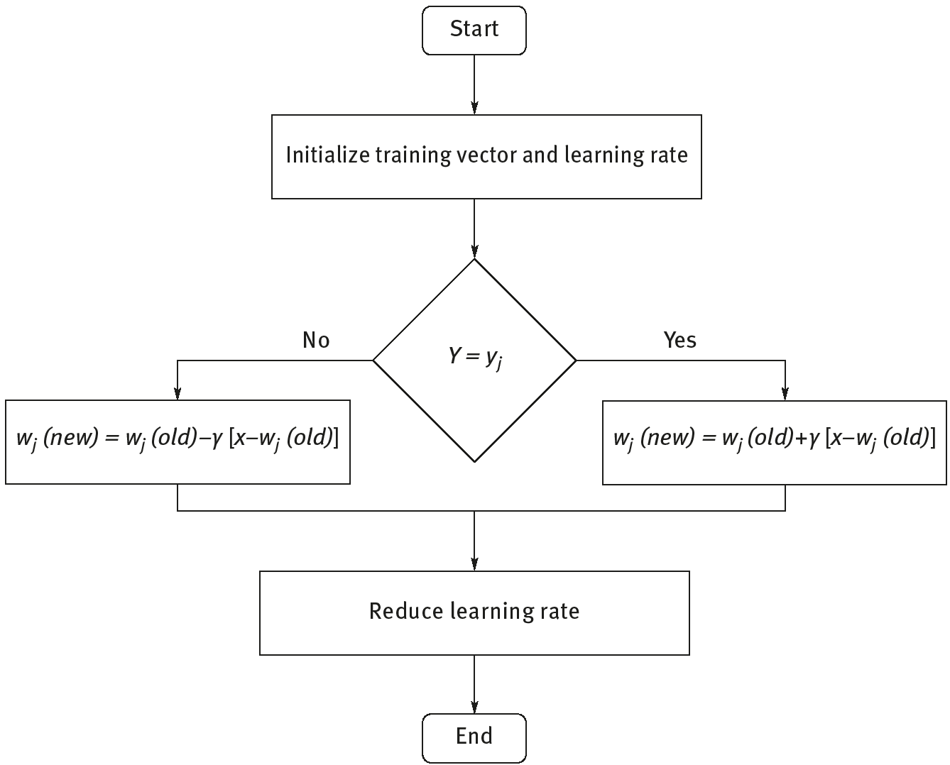
Figure 10.13 shows the steps of LVQ algorithm.
Step (1) Initialize reference vectors (several strategies are discussed shortly). İnitialize learning rate; γ is default (0).
Step (2) While stopping condition is false, follow Steps (2–6).
Step (3) For each training input vector x, follow Steps (3) and (4).

Step (4) Find j so that x −wj is a minimum.
Step (5) Update wij
Steps (6–9) if (Y = yj)
else
Step (10) The condition may postulate a fixed number of iterations (i.e., executions of Step (2)) or learning rate reaching a satisfactorily small value.
A simple method for initializing the weight vectors will be to take the first n training vectors and use them as weight vectors. Each weight vector is calibrated by determining the input patterns that are closest to it. In addition, find the class the largest number of these input patterns belong to and assign that class to the weight vector.
10.3.1LVQ algorithm for the analysis of various data
LVQ algorithmhas been applied on economy (U.N.I.S.) dataset, multiple sclerosis (MS) dataset and WAIS-R dataset in Sections 10.3.1.1, 10.3.1.2 and 10.3.1.3, respectively.
10.3.1.1LVQ algorithm for the analysis of economy (U.N.I.S.)
As the second set of data, we will use, in the following sections, some data related to economies for U.N.I.S. countries. The attributes of these countries’ economies are data regarding years, unemployment, GDP per capita (current international $), youth male (% of male labor force ages 15–24) (national estimate), …, GDP growth (annual%). (Data are composed of a total of 18 attributes.) Data belonging to USA, New Zealand, Italy or Sweden economies from 1960 to 2015 are defined based on the attributes given in Table 2.8 (economy dataset; http://data.worldbank.org) [15], to be used in the following sections. For the classification of D matrix through LVQ algorithm, the first step training procedure is to be employed. For the training procedure, 66.66% of the D matrix can be split for the training dataset (151 × 18), and 33.33% as the test dataset (77 × 18).
Following the classification of the training dataset being trained with LVQ algorithm, we can do the classification of the test dataset. Although the procedural steps of the algorithm may seem complicated at first glance, the only thing you have to do is to concentrate on the steps and grasp them. At this point, we can take a close look at the steps presented in Figure 10.14.
The sample economy data have been selected from countries economies dataset (see Table 2.8) as given in Example 10.1. Let us make the classification based on the economies’ data selected using the steps for Iteration 1 pertaining to LVQ algorithm as shown in Figure 10.14.

Example 10.1 Four vectors are assigned to four classes for economy dataset. The following input vectors represent four classes. In Table 10.13, vector (first column) represents the net domestic credit (current LCU), GDP per capita, PPP (current international $) and GDP growth (annual %) of the subjects on which economies were administered. Class(Y) (second column) represents the USA, New Zealand, Italy and Sweden. Based on the data of the selected economies, the classification of country economy can be done for Iteration 1 of LVQ algorithm as shown in Figure 10.14. Table 10.13 lists economy data normalized with min–max normalization (see Section 3.7, Example 3.4).
Table 10.13: Selected sample from the economy dataset.
| Vector | Class(Y) |
| (1, 4, 2, 0.2) | USA (labeled with 1) |
| (1, 3, 0.9, 0.5) | New Zealand (labeled with 2) |
| (1, 3, 0.5, 0.3) | Italy (labelled with 3) |
| (1, 6, 1, 1) | Sweden (labeled with 4) |
Solution 10.1 Let us do the classification for the LVQ network, with four countries’ economy chosen from economy (U.N.I.S.) dataset. The learning procedure described with vector in LVQ will go on until the minimum error is reached depending on the iteration number. Let us apply the steps of LVQ algorithm as can be seen in Figure 10.14.
Step (1) Initialize w1,w2 weights. Initialize the learning rate γ is 0.1.
Table 10.13 lists the vector data belonging to countries’ economies. LVQ algorithm was applied on them. The related procedural steps are shown in Figure 10.16 and their weight values (w) are calculated.
Iteration 1:
Step (2) Begin computation. For input vector x = (1, 3, 0.9, 0.5) with Y = New Zealand (labeled with 2), do Steps (3) and (4).
Step (3) J = 2, since x is closer to w2 than to w1.
Step (4) Since Y = New Zealand update w2 as follows:
Iteration 2:
Step (2) For input vector x = (1, 4, 2, 0.2) with Y = USA (labeled with 1), do Steps (3) and (4).
Step (4) Since Y = 2 update w1as follows:
Iteration 3:
Step (2) For input vector x = (1, 3, 0.5, 0.3) with Y = Italy (labeled with 3), do Steps (3) and (4).
Step (3) J = 1.
Step (4) Since Y = Italy update w2 as follows:
Step (5) This completes one iteration of training.
Reduce the learning rate.
Step (6) Test the stopping condition.
As a result, the data in the economy dataset with 33.33% portion allocated for the test procedure and classified as USA, New Zealand, Italy and Sweden have been classified with an accuracy rate of 69.6% based on LVQ algorithm.
10.3.1.2LVQ algorithm for the analysis of MS
As presented in Table 2.12 MS dataset has data from the following groups: 76 sample belonging to RRMS, 76 sample to SPMS, 76 sample to PPMS and 76 sample belonging to healthy subjects of control group. The attributes of the control group are data regarding brain stem (MRI 1), corpus callosum periventricular (MRI 2), upper cervical (MRI 3) lesion diameter size (millimetric (mm)) in the MR image and EDSS score. Data are composed of a total of 112 attributes. It is known that using these attributes of 304 individuals, we can know that whether the data belong to the MS subgroup or healthy group. How can we make the classification as to which MS patient belongs to which subgroup of MS including healthy individuals and those diagnosed with MS (based on the lesion diameters (MRI 1, MRI 2 and MRI 3) and number of lesion size for (MRI 1, MRI 2 and MRI 3) as obtained from MRI images and EDSS scores)? D matrix has a dimension of (304 × 112). This means D matrix includes the MS dataset of 304 individuals along with their 112 attributes (see Table 2.12 for the MS dataset). For the classification of D matrix through LVQ algorithm, the first step training procedure is to be employed. For the training procedure, 66.66% of the D matrix can be split for the training dataset (203 × 112) and 33.33%as the test dataset (101 × 112). Following the classification of the training dataset being trained with LVQ algorithm, we can do the classification of the test dataset. Although the procedural steps of the algorithm may seem complicated at the beginning, the only thing you have to do is to concentrate on the steps and comprehend them. At this point, we can take a close look at the steps presented in Figure 10.15.

The sample MS data have been selected from MS dataset (see Table 2.12) in Example 10.2. Let us make the classification based on the MS patients’ data selected using the steps for Iteration 1 pertaining to LVQ algorithm as shown in Figure 10.14.
Example 10.2 Five vectors are assigned to four classes for MS dataset. The following input vectors represent four classes SPMS, PPMS, RRMS and Healthy. In Table 10.14, vector (first column) represents the EDSS, MRI 1 lesion diameter, MRI 2 lesion diameter and MRI 3 lesion diameter of the MS subgroups and healthy data, whereas Class(Y) (second column) represents the MS subgroups and the healthy subjects. Based on the MS patients’ data, the classification of MS subgroup and healthy can be done for Iteration 1 of LVQ algorithm as shown in Figure 10.14.
Solution 10.2 Let us do the classification for the LVQ network, with four MS patients chosen from MS dataset and one healthy individual. The learning procedure described with vector in LVQ will go on till the minimum error is reached depending on the iteration number. Let us apply the steps of LVQ algorithm as can be seen from Figure 10.14 as well.
Table 10.14: Selected sample from the MS dataset as per Table 2.12.
| Vector | Class (Y) |
| (6, 10, 17, 0) | SPMS (labeled with 1) |
| (2, 6, 8, 1) | PPMS (labeled with 2) |
| (6, 15, 30, 2) | RRMS (labeled with 3) |
| (0, 0, 0, 0) | Healthy (labeled with 4) |
Step (1) Initialize w1,w2 weights. Initialize the learning rate γ is 0.1.
In Table 10.14, the LVQ algorithm was applied on the vector data belonging to MS subgroup and healthy subjects. The related procedural steps are shown in Figure 10.15 and accordingly their weight values (w) are calculated.
Iteration 1:
Step (2) Start the calculation. For input vector x = (2, 6, 8, 1) with Y = PPMS (labeled with 2), follow Steps (3) and (4).
Step (3) j = 2, since x is closer to w2 than to w1.
Step (4) Since Y = PPMS update w2 as follows:
Iteration 2:
Step (2) For input vector x = (6, 10, 17, 0) with Y = SPMS (labeled with 1), follow Steps (3) and (4).
Step (3) J = 1
Step (4) Since Y = SPMS update w2 as follows:
Iteration 3:
Step (2) For input vector x = (0, 0, 0, 0) with Y = healthy, follow (labeled with 4) Steps (3) and (4).
Step (3) J = 1
Step (4) Since Y = 2 update w1 as follows:
Steps (3–5) This concludes one iteration of training. Reduce the learning rate.
Step (6) Test the stopping condition.
As a result, the data in the MS dataset with 33.33% portion allocated for the test procedure and classified as RRMS, SPMS, PPMS and healthy have been classified with an accuracy rate of 79.3% based on LVQ algorithm.
10.3.1.3LVQ algorithm for the analysis of mental functions
As presented in Table 2.19, the WAIS-R dataset has data where 200 belong to patient and 200 sample to healthy control group. The attributes of the control group are data regarding school education, gender, …, DM. Data are composed of a total of 21 attributes. It is known that using these attributes of 400 individuals, we can know that whether the data belong to patient or healthy group. How can we make the classification as to which individual belongs to which patient or healthy individuals and those diagnosed with WAIS-R test (based on the school education, gender, the DM, vocabulary, QIV, VIV …, DM)? D matrix has a dimension of 400 × 21. This means D matrix includes the WAIS-R dataset of 400 individuals along with their 21 attributes (see Table 2.19) for the WAIS-R dataset. For the classification of D matrix through LVQ, the first step training procedure is to be employed. For the training procedure, 66.66% of the D matrix can be split for the training dataset (267 × 21) and 33.33% as the test dataset (133 × 21). Following the classification of the training dataset being trained with LVQ algorithm, we classify of the test dataset.
Although the procedural steps of the algorithm may seem complicated at first glance, the only thing you have to do is to concentrate on the steps and grasp them. At this point, we can take a close look at the steps presented in Figure 10.16.
The sample WAIS-R data have been selected from WAIS-R dataset (see Table 2.19) in Example 10.3. Let us make the classification based on the patients’ data selected using the steps for Iteration 1 pertaining to LVQ algorithm in Figure 10.16.
Example 10.3 Three vectors are assigned to two classes for WAIS-R dataset. The following input vectors represent two classes. In Table 10.15, vector (first column) represents the DM, vocabulary, QIV and VIV of the subjects on whom WAIS-R was administered. Class(Y) (second column) represents the patient and healthy subjects. Based on the data of the selected individuals, the classification of WAIS-R patient and healthy can be done for Iteration 1 of LVQ algorithm in Figure 10.16.
Solution 10.3 Let us do the classification for the LVQ network, with two patients chosen from WAIS-R dataset and one healthy individual. The learning procedure described with vector in LVQ will go on until the minimum error is reached depending on the iteration number. Let us apply the steps of LVQ algorithm as can be seen from Figure 10.16.

Step (1) Initialize w1,w2 weights. Initialize the learning rate γ is 0.1.
In Table 10.13, the LVQ algorithm was applied on the vector data belonging to the subjects on whom WAIS-R test was administered. The related procedural steps are shown in Figure 10.16 and accordingly their weight values (w) are calculated.
Iteration 1:
Step (2) Begin computation. For input vector x = (0,0,1,1) with Y = healthy (labeled with 1), do Steps (3) and (4).
Step (3) J = 1, since x is closer to w2 than to w1.
Step (4) Since Y = 1 update w2 as follows:
Iteration 2:
Step (2) For input vector x = (2, 1, 3, 1) with Y = patient, do Steps (3) and (4).
Step (3) J = 1.
Step 4 Since Y = 2 update w2 as follows:
Iteration 3:
Step (2) For input vector x = (4, 6, 4, 1) with Y = patient (labeled with 2), follow Steps (3) and (4).
Step (3) J = 2.
Step (4): Since Y = 2 update w1 as follows:
Steps (3–5) This finalizes one iteration of training. Reduce the learning rate.
Step (6) Test the stopping condition.
As a result, the data in the WAIS-R dataset with 33.33% portion allocated for the test procedure and classified as patient and healthy have been classified with an accuracy rate of 62% based on LVQ algorithm.
References
[1]Hassoun MH. Fundamentals of artificial neural networks. USA: MIT Press, 1995.
[2]Hornik K, Maxwell S, Halbert W. Multilayer feedforward networks are universal approximators. Neural Networks, USA, 1989, 2(5), 359–366.
[3]Annema J, Feed-Forward Neural Networks, New York, USA: Springer Science+Business Media, 1995.
[4]Da Silva IN, Spatti DH, Flauzino RA, Liboni LHB, dos Reis Alves SF. Artificial neural networks. Switzerland: Springer International Publishing, 2017.
[5]Wang SH, Zhang YD, Dong Z, Phillips P. Pathological Brain Detection. Singapore: Springer, 2018.
[6]Trippi RR, Efraim T. Neural networks in finance and investing: Using artificial intelligence to improve real world performance. New York, NY, USA: McGraw-Hill, Inc., 1992.
[7]Rabuñal, JR, Dorado J. Artificial neural networks in real-life applications. USA: IGI Global, 2005.
[8]Graupe D. Principles of artificial neural networks. Advanced series in circuits and systems (Vol. 7), USA: World Scientific, 2013.
[9]Rajasekaran S, Pai GV. Neural networks, fuzzy logic and genetic algorithm: synthesis and applications. New Delhi: PHI Learning Pvt. Ltd., 2003.
[10]Witten IH, Frank E, Hall MA, Pal CJ. Data Mining: Practical machine learning tools and techniques. USA: Morgan Kaufmann Series in Data Management Systems, Elsevier, 2016.
[11]Han J, Kamber M, Pei J, Data mining Concepts and Techniques. USA: The Morgan Kaufmann Series in Data Management Systems, Elsevier, 2012.
[12]Cross SS, Harrison RF, Kennedy RL. Introduction to neural networks. The Lancet, 1995, 346 (8982), 1075–1079.
[13]Kim P. MATLAB Deep Learning: With Machine Learning, Neural Networks and Artificial Intelligence. New York: Springer Science & Business Media, 2017.
[14]Chauvin Y, Rumelhart DE. Backpropagation: Theory, architectures, and applications. New Jersey, USA: Lawrence Erlbaum Associates, Inc., Publishers, 1995.
[15]Karaca Y, Moonis M, Zhang YD, Gezgez C. Mobile cloud computing based stroke healthcare system, International Journal of Information Management, Elsevier, 2018, In Press.
[16]Haykin S. Neural Networks and Learning Machines. New Jersey, USA: Pearson Education, Inc., 2009.
[17]Karaca Y, Cattani. Clustering multiple sclerosis subgroups with multifractal methods and self-organizing map algorithm. Fractals, 2017, 25(4). 1740001.
[18]Karaca Y, Bayrak Ş, Yetkin EF, The Classification of Turkish Economic Growth by Artificial Neural Network Algorithms, In: Gervasi O. et al. (eds) Computational Science and Its Applications, ICCSA 2017. Springer, Lecture Notes in Computer Science, 2017, 10405, 115–126.
[19]Patterson DW. Artificial neural networks: Theory and applications. USA: Prentice Hall PTR, 1998.
[20]Wasserman PD. Advanced methods in neural computing. New York, NY, USA: John Wiley & Sons, Inc., 1993.
[21]Zurada JM. Introduction to artificial neural systems, USA: West Publishing Company, 1992.
[22]Baxt WG. Application of artificial neural networks to clinical medicine. The Lancet, 1995, 346 (8983), 1135–1138.
[23]Kohonen T. Self-organization and associative memory. Berlin Heidelberg: Springer, 1989.
[24]Kohonen T. Self-Organizing Maps. Berlin Heidelberg: Springer-Verlag, 2001.
[25]Kohonen T. Learning vector quantization for pattern recognition. Technical Report TKK-F-A601, Helsinki University of Technology, Department of Technical Physics, Laboratory of Computer and Information Science, 1986.
[26]Kohonen T. Self-Organizing Maps. Berlin Heidelberg: Springer-Verlag, 2001.