
Chapter 7
Understanding and Executing Data Manipulation
This chapter covers Objective 2.3 (Given a scenario, execute data manipulation techniques) of the CompTIA Data+ exam and includes the following topics:
 Data manipulation
- Recoding data
- Derived variables
- Data merging
- Data blending
- Concatenation
- Data appending
- Imputation
- Reduction/aggregation
- Transposing
- Data normalization
- Parsing/string manipulation
For more information on the official CompTIA Data+ exam topics, see the Introduction.
This chapter covers topics related to recoding data, derived variables, data merging, and data blending. It also covers concatenation, data appending, imputation, and reduction/aggregation. Finally, it discusses transposition and normalization of data as well as parsing/string manipulation and data manipulation.
Data Manipulation Techniques
Before we get into the specifics of data manipulation techniques, we need to define a few terms.
For starters, data manipulation refers to the process/methodology of modifying or manipulating data to change it to a more readable and organized format such that it becomes easier for users to consume and work with the data. Data manipulation helps standardize datasets across an organization and enables any business unit to access and store data in a common format.
Data manipulation is an important step for business operations and optimization when dealing with data and analysis. For example, for carrying out consumer behavior analysis or trend analysis, you would want data to be structured in an easy-to-understand format. Table 7.1 gives insights into how data can be possibly structured by age to make it easier to read and process. This is just a sample of how age can be related to needs/wants.
Table 7.1 Data Structured on Needs/Wants According to Age
Age | Category | Needs/Wants |
|---|---|---|
5–12 | Very young | Lollies, gum, toys |
13–18 | Young | Bikes, skates, phones |
19–35 | Adult | Cars, houses, credit cards |
36–55 | Middle-aged | Vacations, investments |
56 and over | Old-aged | Aged care, well-being |
Note
Data Manipulation Language (DML) is a programming language that is used for data manipulation. It helps to amend data, such as by adding, deleting, and changing values in databases, and changes the information so it can be read and understood easily.
Several data manipulation methods are covered in this chapter. Aggregation, sorting, and filtering are the basic functions involved in data manipulation.
Data reconciliation is the verification phase during data migration, in which the destination data is compared with source data to ensure that any issues such as the ones discussed in Chapter 6, “Cleansing and Profiling Data”—for example, missing values, invalid values, and duplicate values—do not impact the data quality.
Recoding Data
Data is comprised of variables. Most of the time, it is necessary to make changes to variables before the data can be analyzed. The process of recoding can be used to transform a current variable into a different one, based on certain criteria and business requirements.
Why should you recode variables rather than use the original variables? It is a best practice to leave the original data unchanged so it can be used again in the future. Instead of changing an original variable, you can recode a variable into a different variable to meet the needs of the organization and maintain the integrity of the original dataset.
Let’s look again at the example from Table 7.1. Let’s say the data is originally structured as shown in Table 7.2.
Table 7.2 Existing Data
Age | Needs/Wants |
|---|---|
5–12 years old | Lollies, gum, toys |
13–18 years old | Bikes, skates, phones |
19–35 years old | Cars, houses, credit cards |
36–55 years old | Vacations, investments |
56 years of age and over | Aged care, well-being |
Now, to make sense of the ages expressed in years, this data can be recoded in the format outlined in Table 7.3 (which is very similar to Table 7.1).
Table 7.3 Recoded Data: From Ages in Numbers of Years to Categorical Age Groups
Age (Years) | New Recoded Category (Age Groups) | Needs/Wants |
|---|---|---|
5–12 | Very young | Lollies, gum, toys |
13–18 | Young | Bikes, skates, phones |
19–35 | Adult | Cars, houses, credit cards |
36–55 | Middle-aged | Vacations, investments |
56 and over | Old-aged | Aged care, well-being |
As you can see, instead of explaining to someone what constitutes young and adult or the age range between middle-aged and old-aged, it is easier to recode from numeric values into categorical strings that clearly segregate one age group from another and their needs/wants. Essentially, if the original data was as expressed in Table 7.2, after recoding it will be as shown in Table 7.3 (almost a replica of Table 7.1) that’s easier to comprehend.
Recoding is typically used for merging categories of variables into fewer groups or different groups—as in the previous example, where we recoded data into different (categorical) groups. Recoding can be done with the same or different variables.
Data management and analytics tools such as IBM Statistical Package for the Social Sciences (SPSS) offer solutions to recode data from one variable to another variable (see Figure 7.1).

Figure 7.1 Recoding Options in the Transform Menu of IBM SPSS
There are two main options for recoding data: recoding numeric values or recoding categorical data.
Recoding categorical variables can be useful, for example, if there is a need to use fewer or combined categories than were used in collecting the data. Again using our example of age groups, we could recode categorically as shown in Table 7.4.
Table 7.4 Recoding Categorical Values
Age (Years) | Age Groups |
|---|---|
5–18 | Young |
19–35 | Adult |
36–55 | Middle-aged |
56 and over | Old-aged |
Here, we have collapsed the categories very young and young, which are closely aligned, into young by collating the two categories. We have done this because the organization may want to look at this as one broad category.
To see an example of recoding numeric values, consider Table 7.5, which assigns numeric values to sex of an individual.
Table 7.5 Assigning Numerical Values to Sex
Value | Sex |
|---|---|
0 | Unidentified |
1 | Male |
2 | Female |
3 | Undisclosed |
If the organization does not need to distinguish between the unidentified and undisclosed sex options, we can recode these numeric values as shown in Table 7.6.
Table 7.6 Recoding Numerical Values
Value | Sex |
|---|---|
0 | Male |
1 | Female |
2 | Other |
As you can see, whereas 0 was used for unidentified in Table 7.5, it is used for male in Table 7.6. Similarly, 1 was used for male earlier but is now used for female. The new variable other has been assigned to the number 3.
Derived Variables
As the name suggests, derived variables are variables derived from existing variables. In other words, a derived variable is defined by a parameter or an expression related to existing variables in a dataset. For example, if the existing variable is product_manufacture_date, a derived variable could be day_and_time_of_manufacturing or best_before_date.
To put this in context, let’s consider an example. Say that every soft drink has a manufacturing or production date, such as:
product_manufacture_date = 24/10/2022
It also has a best before date, as well as an optional time of manufacturing, such as:
best_before_date = 24/10/2023
day_and_time_of_manufacturing = Monday, 11:34 am
It is quite obvious that any derived variables would be used in a similar fashion as any other variable. Because they are dependent on the variables from which they’re derived, any change in the value of the original variable will change the values of the derived variable as well. Again, let’s look at our previous soft drink example, in this case the variable being changed is the manufacturing date and hence, the best before date also changes accordingly:
product_manufacture_date = 24/11/2022
best_before_date = 24/11/2023
day_and_time_of_manufacturing = Thursday, 11:20 am
Data Merges
A data merge (as the name indicates) is a technique for merging two or more similar datasets into one (larger) dataset. Data merge is mostly leveraged for ease of data analysis; if you merge multiple datasets into one larger dataset, you can then run queries on all the data at once. Figure 7.2 shows the data merge process between two datasets (in this case, tables).

Figure 7.2 Data Merge
There are two main types of data merge operations:
 Appending data: This type of merge involves adding rows. For example, Figure 7.2 shows new rows being added to perform a data merge.
- Merging in new variables: A data merge accomplished by adding new variables implies adding new columns in the table or the new merged dataset.
Data Blending
Data blending is all about combining data from multiple data sources to create a new dataset. Data blending is very similar to data merging, but it brings together data from multiple sources that may be very dissimilar. Data blending allows an organization to bring together data from the Internet, spreadsheets, ERP, CRM, and other applications in order to present the data in a dashboard or another visualization (such as a report) for analysis.
Why not analyze the data separately and then bring together the analysis in one place? The simple answer is that not every organization has the required resources—such as data scientists and advanced analytics tools—at its disposal. In addition, organizations are often looking for rather simple views of data patterns to drive sales or marketing rather than mining deeply.
Blending of data allows a data analyst to incorporate information from almost any data sources for analysis and makes possible deeper and faster business insights. Data blending tools enable faster data-driven decision making by creating a reporting dashboard that automatically populates with real-time data, offering much better and more intuitive insights compared to using multiple reports. With a dashboard, data insights can be focused on a specific problem statement.
The high-level steps in data blending are as follows:
Prepare the data. This step involves determining pertinent datasets from well-known data sources and transforming different datasets into a general structure that helps form a meaningful blend.
Blend the data. This step allows blending the data from different data sources and customizing each blend based on the common dimension to ensure that the blending of data is meaningful (that is, the data being blended is in the context of the problem being solved).
Validate outcomes. As blending from multiple sources can potentially lead to inaccuracies, the data is examined for any inconsistencies as well as any missing information. If required, the data might need to be cleansed and (re)formatted.
Store and visualize the data. After data blending is completed, the data can be stored in the destination data store. Organizations can leverage business intelligence tools to create dashboards and/or reports. Visualization tools such as Tableau may be used for generating dashboards. The tool chosen depends on the reason data blending was performed and the specific problem being solved.
Concatenation
Concatenation (often shortened to concat) is a function or an operation that makes it possible to combine string, text, numeric, or other data from two or more fields in a dataset. Concatenation allows you to merge multiple cells, whether they involve text or numbers, without disturbing the original cells.
Figure 7.3 shows the CONCATENATE function in Microsoft Excel.

Figure 7.3 Concatenation in Microsoft Excel
Figure 7.3 shows an example of trying to concatenate the first name and last name, with a space in between. Figure 7.4 shows the outcome of this concatenation.
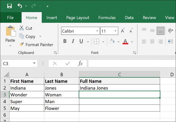
Figure 7.4 Outcome of Concatenation in Microsoft Excel
Figure 7.5 shows the final outcome when the same function is applied across all fields in the table.
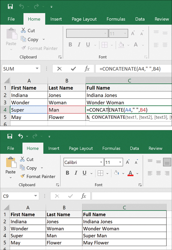
Figure 7.5 Concatenation Output Across the Table
Note
Concatenation allows you to combine various data types, like text, strings, and num-bers, which is quite difficult to do without a dedicated function.
The key benefit of concatenation is that there is no need to change the data source; rather, you refer to the data source. When the original information is changed, the information in the combined cell gets automatically updated.
Data Appending
Another key data manipulation technique is data appending, where new data elements are added to an existing dataset or database. Think of data appending as supplementing an existing database by leveraging data from other databases to fill in the gaps, such as missing information.
Why should you focus on data appending? There are multiple benefits to data appending, including:
- Clean and precise customer records that help with personalized customer approach and interaction
- Improved customer acquisition via focused omnichannel marketing campaigns
- Reduced data management costs and enhanced data quality
Data appending might be used to enrich an organization’s customer database that is missing records like emails or contact information. For example, by matching records against one or more external databases, you can find the desired missing data fields and then add them to your organization’s customer database. Data appending is often leveraged to ensure that a sales or marketing strategy is well defined based on the customer data view, such as for running an email campaign for lead generation.
Note
Data appending should be completed to gain the information and insights needed to carry out an organization’s overall strategy. However, it does not form part of the strategy itself; instead, it helps identify a baseline to develop a good overall picture of how these efforts can be concentrated.
Figure 7.6 shows the append queries in Microsoft Excel.

Figure 7.6 Appending in Microsoft Excel
Figure 7.7 shows the Power Query Editor, where you can append rows into one table. It shows an example of trying to append the sales funnel with tagged deals.
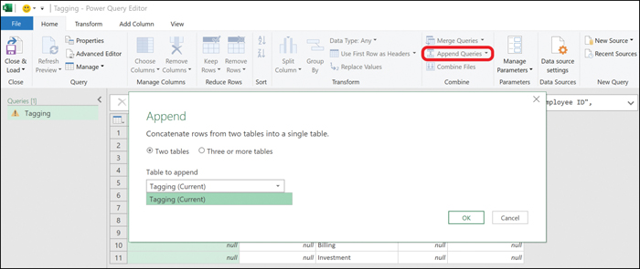
Figure 7.7 Appending Queries in Microsoft Excel
At a very high level, the following steps are involved in data appending:
Normalize the existing data and remove any extraneous data.
Set up a validation process to ensure that database fields are correct after appending.
Match the existing database with parallel entries in an external database.
Select which data fields/attributes need to be appended (for example, email, physical address).
Use the selected fields/attributes to append the existing records.
Imputation
We briefly touched on imputation, which is the process of replacing missing values, in Chapter 6. Figure 7.8 shows an overview of imputation.

Figure 7.8 Imputation of Missing Values
Missing data maximizes the probability of making type II and type I errors and reduces the accuracy of statistical outcomes.
Note
Type I and type II errors are discussed in Chapter 10.
Imputation fills in missing values rather than altogether removing the variables or fields that are missing data. While imputation helps keep the full sample size, which can be advantageous for accuracy from a statistical perspective, the imputed values may yield different kinds of bias.
Imputation can be broadly categorized as single imputation or multiple imputation. With single imputation, a missing value is replaced by a value defined by a certain rule or logic. In contrast, with multiple imputation, multiple values are used to substitute missing values.
The various types of imputation that can be used for substituting missing values are as follows:
- Imputation based on related observations: This is useful when there are large data samples available to substitute similar (though not exact) values. For example, it is possible to use data on weight and height in adults in a certain population to fill in missing values in another population. Such imputations, however, could lead to measurement errors.
- Imputation based on logical rules: At times it is possible to impute using logical rules, such as the number of hours worked and the cost of labor based on a survey conducted with 10,000 workers. Some respondents might give input on how much they earn per hour for a particular job role; however, 1,000 of the respondents might refuse to answer the earnings question, and thus it is possible to impute zero earnings to these. Logic is important here: If we use 0 as the default filler for nonrespondents, their income is getting recorded as nothing, possibly affecting the sample.
- Imputation based on creating a new variable category: In some cases, it is useful to use imputation to add a new/extra category or group for the variable(s) that may be missing.
- Imputation based on the last observation carried forward: With this method, which is typically applicable to time series data, the substitutions are performed by using the pretreated data (that is, using the last observed value of a participant or respondent as a substitute for that individual’s missing values).
Data Reduction
Imagine a number of huge datasets coming from different data warehouses for analysis. Data analysts would have a hard time dealing with that volume of data, especially when running complex queries on such a huge amount of data. Complex queries take a long time to execute. Data reduction, also known as data aggregation, is really useful at reducing complexity.
Data reduction is a data manipulation technique that is used to minimize the size of a dataset by aggregating, clustering, or removing any redundant features. Even though the data size is reduced—which is great for analysis—it yields the same analytical outcomes.
The following are some of the common ways data reduction is achieved:
- Data compression: Data transformation is applied to the original data to compress the data. You are likely to compress data by zipping up a file or reducing the size of an image on your PC. If the file can be retrieved without any loss, data compression was lossless; however, if the data cannot be retrieved without loss, the compression is considered lossy in nature.
- Dimensionality reduction: This method leverages encoding to reduce the volume of the original data by removing unwanted attributes. Like data compression, dimensionality reduction can be lossy or lossless. An example of a dimensionality reduction technique is wavelet transformation.
- Numerosity reduction: This method reduces the volume of the original data to a smaller form of data—such as a data model instead of the actual data. There are two types of numerosity reduction: parametric (for example, log-linear and regression models) and non-parametric (for example, sampling and clustering) numerosity reduction.
Data Transposition
Data transposition involves rotating the data from a column to a row or rotating the data from a row to a column. For example, Figure 7.9 shows an Excel worksheet with the current setup for product sales by region across Q1, Q2, Q3, and Q4. Here the quarters are across rows and regions are across columns.

Figure 7.9 Original Sales by Region Table
By using the TRANSPOSE function, you can transpose rows to columns and columns to rows. You do this by copying the existing table, right-clicking anywhere in sheet, and choosing Transpose under the Paste options (see Figure 7.10). Excel swaps the rows and columns.

Figure 7.10 Transposing Data in Excel
Why would you want to transpose data? Changing the layout of data might make the data simpler to understand and work with. Going by the regions across rows and looking at quarterly sales revenues may be easier to interpret.
Normalizing Data
ExamAlert
Normalization is a fundamental concept used in data redundancy reduction, and you can expect to be tested on this topic on the CompTIA Data+ exam.
The main aim of normalization, as mentioned in Chapter 6, is to remove repetitive (or redundant) information from a database and ensure that information is logically stored (that is, ensure that only related data is stored in a table).
Note
The goal of normalization is to reduce data redundancy by eliminating insertion, updating, and deleting anomalies.
Following are the five normal forms (NF):
- First normal form (1NF)
- Second normal form (2NF)
- Third normal form (3NF)
- Boyce–Codd normal form (BCNF), or 3.5 normal form (3.5NF)
- Fourth normal form (4NF)
For a table to be in first normal form, it should follow these rules:
- It should only have single-valued attributes/columns. In other words, duplicate columns should be eliminated from the table.
- Separate tables should be created for each group of related data with their own primary keys.
For a table to be in 2NF, it should follow these rules:
- The table should meet the requirements of 1NF.
- The table should not have partial dependencies, and you should create relationships between this table and other tables through the use of foreign keys.
For a table to be in 3NF, it should follow these rules:
- The table should meet the requirements of 2NF.
- The table must not have transitive dependency, so you should remove the columns that are not dependent on the primary key.
For a table to be in 3.5NF, it should follow these rules:
- The table should meet the requirements of 3NF.
- The table should not have multiple overlapping candidate keys.
For a table to be in 4NF, it should follow these rules:
- The table should meet the requirements of 3.5NF.
- The table must not have multivalued dependencies.
Parsing/String Manipulation
It is very common to have semi-structured and unstructured data stored in strings. You are therefore likely to be required to deal with string manipulation for data analysis. String manipulation involves handling and analyzing strings and might include operations such as splicing, changing, parsing, pasting, and analyzing strings to be able to use the information stored in the strings.
Filtering
When working with a large amount of data, it can be difficult to explore the key aspects that may be of interest due to the presence of non-required data (or noise). It is very common for data analysts to leverage data filters to better analyze data. As data is filtered, only the rows or columns that meet the filter criteria are displayed, and other (less relevant) rows or columns are hidden.
By applying the filter in Figure 7.11, you can filter the data by state. Figure 7.12, for instance, shows a filter to show all orders for the state of Arizona. This filter helps prune irrelevant orders.

Figure 7.11 Unfiltered Data in Excel
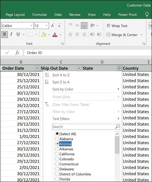
Figure 7.12 Filtering Data in Excel
Sorting
Data manipulation can be done in various ways, and one of the easiest ways is to sort the data in such a way that it becomes more readable or usable. For example, you can use the built-in sorting function in Microsoft Excel to sort data in a few ways (see Figure 7.13):
- From oldest to newest or newest to oldest (based on numerical values)
- From A to Z or Z to A (based on alphanumerical values)
- Using a custom sort

Figure 7.13 Data Sorting Options in Excel
Sorting is typically applied on a column to sort the data in either ascending or descending order. This gives insight to the applicable data across all rows, as per the chosen sorting option.
When using the custom sort, you can choose the sort value(s) according to the sorting order you want to apply, as shown in Figure 7.14.

Figure 7.14 Custom Sorting Options in Excel
Date Functions
Datasets often include dates. SQL queries give you the power to manipulate information related to dates and times. For example, MySQL provides the time and date functions shown in Table 7.7.
Table 7.7 MySQL Date Functions
Function | Output |
|---|---|
Select CURDATE(); | The current date |
Select CURTIME(); | The current time |
Select NOW(); | The current date and time |
DATEDIFF(date1, date2) | The number of days between two dates |
DATE_FORMAT(date, format); | The date/time in a different format |
Figure 7.15 shows some of these MySQL queries executed using MySQL Workbench as the front end and Azure Database for MySQL as the back end.

Figure 7.15 MySQL Data Function Queries
Logical Functions
When working with data values, you may want to ascertain whether a condition leads to true or false output. In such a case, you can leverage logical functions to evaluate a given expression against a list of values to get positive (true) or negative (false) output. For example, say that there are two values, A and B, where:
A = 200
B = 100
The simplest expressions might be A > B is true while A < B is false. However, when dealing with complex expressions, you need logical functions, including:
- AND
- OR
- NOT
- IF
Let’s look at how to leverage the power of Microsoft Excel with logical functions and the two values A and B that we just defined. In Figure 7.16, you can see the expression =AND(A1>50,B1>50). When you press Enter, you should get the answer TRUE.
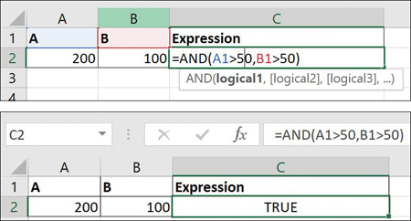
Figure 7.16 AND Logical Function in Excel
In this case, the logical operator AND is evaluating all criteria to give the output. In this case, because both values are greater than 50, the answer is TRUE. Now if we set B1<50, we get the outcome shown in Figure 7.17.

Figure 7.17 AND Logical Function in Excel, Continued
Now, because B1 is greater than 50, that part of the expression is false; therefore, AND leads to the outcome FALSE.
What happens if we keep the expression the same except that we change AND to OR, so that the expression now reads =OR(A1>50,B1<50)? What do you think the output would be? Figure 7.18 shows the answer.

Figure 7.18 OR Logical Function in Excel
The NOT function simply reverses the value from TRUE to FALSE and from FALSE to TRUE, as shown in Figure 7.19.

Figure 7.19 NOT Logical Function in Excel
The TRUE function (that is, =TRUE()) returns the logical TRUE value, and the FALSE function (that is, =FALSE()) returns the logical FALSE value.
The Excel IF logical function makes it possible to create logical comparisons and has two possible outcomes. That is, if the comparison is TRUE, the first result is returned; if the comparison is FALSE, the second result is returned (see Figure 7.20).

Figure 7.20 IF Logical Function in Excel
Note
For a comprehensive list of all Microsoft Excel logical functions, see https://support.microsoft.com/en-us/office/logical-functions-reference-e093c192-278b-43f6-8c3a-b6ce299931f5.
Aggregate Functions
The word aggregate implies bringing together or summarizing. In the context of databases, aggregation implies bringing together/grouping the values of rows. The commonly used SQL aggregate functions are:
- SUM(): This function returns the sum of all values in a particular column.
- AVG(): This function returns the average value of a particular column.
- COUNT(): This function returns the total number of rows matching the query.
- MAX(): This function returns the largest value in a particular column.
- MIN(): This function returns the smallest value in a particular column.
To illustrate a few of the aggregation functions, the following examples run queries in MySQL Workbench against the sample database available at https://github.com/Azure-Samples/mysql-database-samples/blob/main/mysqltutorial.org/mysql-classicmodesl.sql.
Figure 7.21 shows the following COUNT() aggregation query:
SELECT COUNT(contactFirstName) FROM customers
WHERE state = "NY";

Figure 7.21 COUNT() Query in MySQL
Figure 7.22 shows the following AVG() aggregation query:
SELECT avg(creditLimit) FROM customers;

Figure 7.22 AVG() Query in MySQL
Figure 7.23 shows the following MAX() aggregation query:
SELECT max(creditLimit) FROM customers;

Figure 7.23 MAX() Query in MySQL
System Functions
System functions are functions that make changes to the database structure or information stored in the database (for example, adding a new row or inputting a new data value in a cell). The key SQL functions that can be used to change the information or structure of a database table are:
- INSERT: This function enables database administrators/users to add new rows to an existing table.
- UPDATE: This function enables database administrators/users to update the data of an existing table in a database.
- DELETE: This function enables database administrators/users to remove existing records from existing tables.
For example, this query inserts values into the sample database:
insert into customers values (103,'Atelier,'Schmitt','Carine ',
'40.32.2555','54, rue Royale',NULL,'Nantes',NULL,'44000',
'France',1370,'21000.00');What Next?
If you want more practice on this chapter’s exam objective before you move on, remember that you can access all of the Cram Quiz questions on the Pearson Test Prep software online. You can also create a custom exam by objective with the Online Practice Test. Note any objective you struggle with and go to that objective’s material in this chapter.