Chapter 9 Atomics
In the first half of the book, we saw many occasions where something complicated to accomplish with a single-threaded application becomes quite easy when implemented using CUDA C. For example, thanks to the behind-the-scenes work of the CUDA runtime, we no longer needed for() loops in order to do per-pixel updates in our animations or heat simulations. Likewise, thousands of parallel blocks and threads get created and automatically enumerated with thread and block indices simply by calling a __global__ function from host code.
On the other hand, there are some situations where something incredibly simple in single-threaded applications actually presents a serious problem when we try to implement the same algorithm on a massively parallel architecture. In this chapter, we’ll take a look at some of the situations where we need to use special primitives in order to safely accomplish things that can be quite trivial to do in a traditional, single-threaded application.
9.1 Chapter Objectives
Through the course of this chapter, you will accomplish the following:
• You will learn about the compute capability of various NVIDIA GPUs.
• You will learn about what atomic operations are and why you might need them.
• You will learn how to perform arithmetic with atomic operations in your CUDA C kernels.
9.2 Compute Capability
All of the topics we have covered to this point involve capabilities that every CUDA-enabled GPU possesses. For example, every GPU built on the CUDA Architecture can launch kernels, access global memory, and read from constant and texture memories. But just like different models of CPUs have varying capabilities and instruction sets (for example, MMX, SSE, or SSE2), so too do CUDA-enabled graphics processors. NVIDIA refers to the supported features of a GPU as its compute capability.
9.2.1 The Compute Capability of NVIDIA GPUs
As of press time, NVIDIA GPUs could potentially support compute capabilities 1.0, 1.1, 1.2, 1.3, or 2.0. Higher-capability versions represent supersets of the versions below them, implementing a “layered onion” or “Russian nesting doll” hierarchy (depending on your metaphorical preference). For example, a GPU with compute capability 1.2 supports all the features of compute capabilities 1.0 and 1.1. The NVIDIA CUDA Programming Guide contains an up-to-date list of all CUDA-capable GPUs and their corresponding compute capability. Table 9.1 lists the NVIDIA GPUs available at press time. The compute capability supported by each GPU is listed next to the device’s name.
Table 9.1 Selected CUDA-Enabled GPUs and Their Corresponding Compute Capabilities
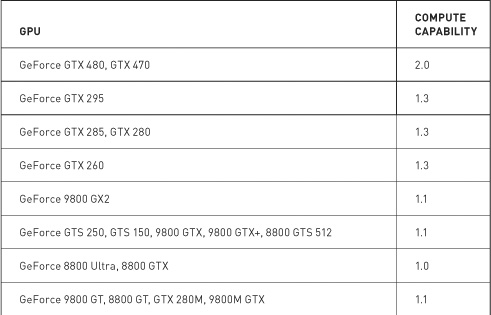
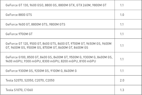
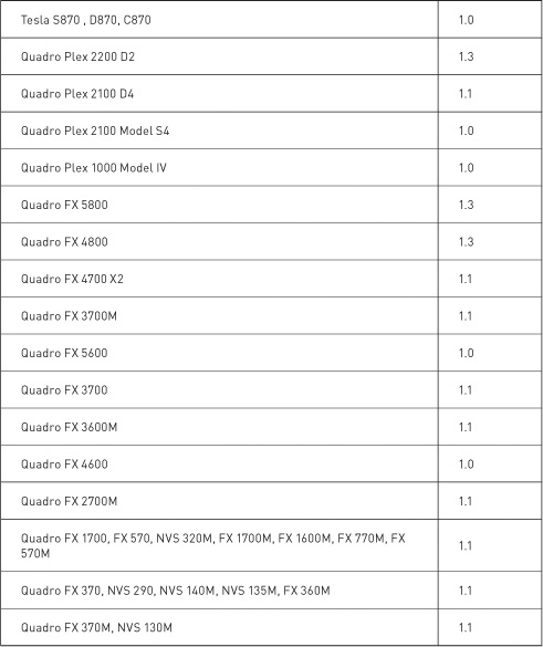
Of course, since NVIDIA releases new graphics processors all the time, this table will undoubtedly be out-of-date the moment this book is published. Fortunately, NVIDIA has a website, and on this website you will find the CUDA Zone. Among other things, the CUDA Zone is home to the most up-to-date list of supported CUDA devices. We recommend that you consult this list before doing anything drastic as a result of being unable to find your new GPU in Table 9.1. Or you can simply run the example from Chapter 3 that prints the compute capability of each CUDA device in the system.
Because this is the chapter on atomics, of particular relevance is the hardware capability to perform atomic operations on memory. Before we look at what atomic operations are and why you care, you should know that atomic operations on global memory are supported only on GPUs of compute capability 1.1 or higher. Furthermore, atomic operations on shared memory require a GPU of compute capability 1.2 or higher. Because of the superset nature of compute capability versions, GPUs of compute capability 1.2 therefore support both shared memory atomics and global memory atomics. Similarly, GPUs of compute capability 1.3 support both of these as well.
If it turns out that your GPU is of compute capability 1.0 and it doesn’t support atomic operations on global memory, well maybe we’ve just given you the perfect excuse to upgrade! If you decide you’re not ready to splurge on a new atomics-enabled graphics processor, you can continue to read about atomic operations and the situations in which you might want to use them. But if you find it too heartbreaking that you won’t be able to run the examples, feel free to skip to the next chapter.
9.2.2 Compiling for a Minimum Compute Capability
Suppose that we have written code that requires a certain minimum compute capability. For example, imagine that you’ve finished this chapter and go off to write an application that relies heavily on global memory atomics. Having studied this text extensively, you know that global memory atomics require a compute capability of 1.1. To compile your code, you need to inform the compiler that the kernel cannot run on hardware with a capability less than 1.1. Moreover, in telling the compiler this, you’re also giving it the freedom to make other optimizations that may be available only on GPUs of compute capability 1.1 or greater. Informing the compiler of this is as simple as adding a command-line option to your invocation of nvcc:
nvcc -arch=sm_11
Similarly, to build a kernel that relies on shared memory atomics, you need to inform the compiler that the code requires compute capability 1.2 or greater:
nvcc -arch=sm_12
9.3 Atomic Operations Overview
Programmers typically never need to use atomic operations when writing traditional single-threaded applications. If this is the situation with you, don’t worry; we plan to explain what they are and why we might need them in a multithreaded application. To clarify atomic operations, we’ll look at one of the first things you learned when learning C or C++, the increment operator:
x++;
This is a single expression in standard C, and after executing this expression, the value in x should be one greater than it was prior to executing the increment. But what sequence of operations does this imply? To add one to the value of x, we first need to know what value is currently in x. After reading the value of x, we can modify it. And finally, we need to write this value back to x.
So the three steps in this operation are as follows:
1. Read the value in x.
2. Add 1 to the value read in step 1.
3. Write the result back to x.
Sometimes, this process is generally called a read-modify-write operation, since step 2 can consist of any operation that changes the value that was read from x.
Now consider a situation where two threads need to perform this increment on the value in x. Let’s call these threads A and B. For A and B to both increment the value in x, both threads need to perform the three operations we’ve described. Let’s suppose x starts with the value 7. Ideally we would like thread A and thread B to do the steps shown in Table 9.2.
Table 9.2 Two threads incrementing the value in x
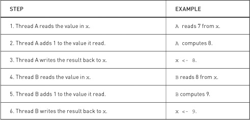
Since x starts with the value 7 and gets incremented by two threads, we would expect it to hold the value 9 after they’ve completed. In the previous sequence of operations, this is indeed the result we obtain. Unfortunately, there are many other orderings of these steps that produce the wrong value. For example, consider the ordering shown in Table 9.3 where thread A and thread B’s operations become interleaved with each other.
Table 9.3 Two threads incrementing the value in x with interleaved operations
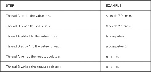
Therefore, if our threads get scheduled unfavorably, we end up computing the wrong result. There are many other orderings for these six operations, some of which produce correct results and some of which do not. When moving from a single-threaded to a multithreaded version of this application, we suddenly have potential for unpredictable results if multiple threads need to read or write shared values.
In the previous example, we need a way to perform the read-modify-write without being interrupted by another thread. Or more specifically, no other thread can read or write the value of x until we have completed our operation. Because the execution of these operations cannot be broken into smaller parts by other threads, we call operations that satisfy this constraint as atomic. CUDA C supports several atomic operations that allow you to operate safely on memory, even when thousands of threads are potentially competing for access.
Now we’ll take a look at an example that requires the use of atomic operations to compute correct results.
9.4 Computing Histograms
Oftentimes, algorithms require the computation of a histogram of some set of data. If you haven’t had any experience with histograms in the past, that’s not a big deal. Essentially, given a data set that consists of some set of elements, a histogram represents a count of the frequency of each element. For example, if we created a histogram of the letters in the phrase Programming with CUDA C, we would end up with the result shown in Figure 9.1.
Figure 9.1 Letter frequency histogram built from the string Programming with CUDA C
![]()
Although simple to describe and understand, computing histograms of data arises surprisingly often in computer science. It’s used in algorithms for image processing, data compression, computer vision, machine learning, audio encoding, and many others. We will use histogram computation as the algorithm for the following code examples.
9.4.1 CPU Histogram Computation
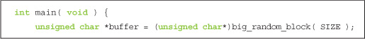
Because the computation of a histogram may not be familiar to all readers, we’ll start with an example of how to compute a histogram on the CPU. This example will also serve to illustrate how computing a histogram is relatively simple in a single-threaded CPU application. The application will be given some large stream of data. In an actual application, the data might signify anything from pixel colors to audio samples, but in our sample application, it will be a stream of randomly generated bytes. We can create this random stream of bytes using a utility function we have provided called big_random_block(). In our application, we create 100MB of random data.

Since each random 8-bit byte can be any of 256 different values (from 0x00 to 0xFF), our histogram needs to contain 256 bins in order to keep track of the number of times each value has been seen in the data. We create a 256-bin array and initialize all the bin counts to zero.

Once our histogram has been created and all the bins are initialized to zero, we need to tabulate the frequency with which each value appears in the data contained in buffer[]. The idea here is that whenever we see some value z in the array buffer[], we want to increment the value in bin z of our histogram. This way, we’re counting the number of times we have seen an occurrence of the value z.
If buffer[i] is the current value we are looking at, we want to increment the count we have in the bin numbered buffer[i]. Since bin buffer[i] is located at histo[buffer[i]], we can increment the appropriate counter in a single line of code.
histo[buffer[i]]++;
We do this for each element in buffer[] with a simple for() loop:

At this point, we’ve completed our histogram of the input data. In a full application, this histogram might be the input to the next step of computation. In our simple example, however, this is all we care to compute, so we end the application by verifying that all the bins of our histogram sum to the expected value.

If you’ve followed closely, you will realize that this sum will always be the same, regardless of the random input array. Each bin counts the number of times we have seen the corresponding data element, so the sum of all of these bins should be the total number of data elements we’ve examined. In our case, this will be the value SIZE.
And needless to say (but we will anyway), we clean up after ourselves and return.

On our benchmark machine, a Core 2 Duo, the histogram of this 100MB array of data can be constructed in 0.416 seconds. This will provide a baseline performance for the GPU version we intend to write.
9.4.2 GPU Histogram Computation
We would like to adapt the histogram computation example to run on the GPU. If our input array is large enough, it might save a considerable amount of time to have different threads examining different parts of the buffer. Having different threads read different parts of the input should be easy enough. After all, it’s very similar to things we have seen so far. The problem with computing a histogram from the input data arises from the fact that multiple threads may want to increment the same bin of the output histogram at the same time. In this situation, we will need to use atomic increments to avoid a situation like the one described in Section 9.3: Atomic Operations Overview.
Our main() routine looks very similar to the CPU version, although we will need to add some of the CUDA C plumbing in order to get input to the GPU and results from the GPU. However, we start exactly as we did on the CPU:
We will be interested in measuring how our code performs, so we initialize events for timing exactly like we always have.

After setting up our input data and events, we look to GPU memory. We will need to allocate space for our random input data and our output histogram. After allocating the input buffer, we copy the array we generated with big_random_block() to the GPU. Likewise, after allocating the histogram, we initialize it to zero just like we did in the CPU version.

You may notice that we slipped in a new CUDA runtime function, cudaMemset(). This function has a similar signature to the standard C function memset(), and the two functions behave nearly identically. The difference in signature between these functions is that cudaMemset() returns an error code while the C library function memset() does not. This error code will inform the caller whether anything bad happened while attempting to set GPU memory. Aside from the error code return, the only difference is that cudaMemset() operates on GPU memory while memset() operates on host memory.
After initializing the input and output buffers, we are ready to compute our histogram. You will see how we prepare and launch the histogram kernel momentarily. For the time being, assume that we have computed the histogram on the GPU. After finishing, we need to copy the histogram back to the CPU, so we allocate a 256-entry array and perform a copy from device to host.

At this point, we are done with the histogram computation so we can stop our timers and display the elapsed time. Just like the previous event code, this is identical to the timing code we’ve used for several chapters.

At this point, we could pass the histogram as input to another stage in the algorithm, but since we are not using the histogram for anything else, we will simply verify that the computed GPU histogram matches what we get on the CPU. First, we verify that the histogram sum matches what we expect. This is identical to the CPU code shown here:

To fully verify the GPU histogram, though, we will use the CPU to compute the same histogram. The obvious way to do this would be to allocate a new histogram array, compute a histogram from the input using the code from Section 9.4.1: CPU Histogram Computation, and, finally, ensure that each bin in the GPU and CPU version match. But rather than allocate a new histogram array, we’ll opt to start with the GPU histogram and compute the CPU histogram “in reverse.”
By computing the histogram “in reverse,” we mean that rather than starting at zero and incrementing bin values when we see data elements, we will start with the GPU histogram and decrement the bin’s value when the CPU sees data elements. Therefore, the CPU has computed the same histogram as the GPU if and only if every bin has the value zero when we are finished. In some sense, we are computing the difference between these two histograms. The code will look remarkably like the CPU histogram computation but with a decrement operator instead of an increment operator.

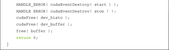
As usual, the finale involves cleaning up our allocated CUDA events, GPU memory, and host memory.

Before, we assumed that we had launched a kernel that computed our histogram and then pressed on to discuss the aftermath. Our kernel launch is slightly more complicated than usual because of performance concerns. Because the histogram contains 256 bins, using 256 threads per block proves convenient as well as results in high performance. But we have a lot of flexibility in terms of the number of blocks we launch. For example, with 100MB of data, we have 104,857,600 bytes of data. We could launch a single block and have each thread examine 409,600 data elements. Likewise, we could launch 409,600 blocks and have each thread examine a single data element.
As you might have guessed, the optimal solution is at a point between these two extremes. By running some performance experiments, optimal performance is achieved when the number of blocks we launch is exactly twice the number of multiprocessors our GPU contains. For example, a GeForce GTX 280 has 30 multiprocessors, so our histogram kernel happens to run fastest on a GeForce GTX 280 when launched with 60 parallel blocks.
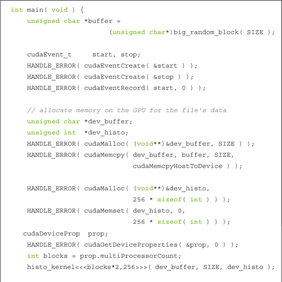
In Chapter 3, we discussed a method for querying various properties of the hardware on which our program is running. We will need to use one of these device properties if we intend to dynamically size our launch based on our current hardware platform. To accomplish this, we will use the following code segment. Although you haven’t yet seen the kernel implementation, you should still be able to follow what is going on.
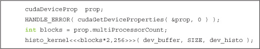
Since our walk-through of main() has been somewhat fragmented, here is the entire routine from start to finish:

Histogram Kernel Using Global Memory Atomics
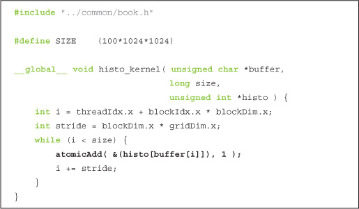
And now for the fun part: the GPU code that computes the histogram! The kernel that computes the histogram itself needs to be given a pointer to the input data array, the length of the input array, and a pointer to the output histogram. The first thing our kernel needs to compute is a linearized offset into the input data array. Each thread will start with an offset between 0 and the number of threads minus 1. It will then stride by the total number of threads that have been launched. We hope you remember this technique; we used the same logic to add vectors of arbitrary length when you first learned about threads.

Once each thread knows its starting offset i and the stride it should use, the code walks through the input array incrementing the corresponding histogram bin.

The highlighted line represents the way we use atomic operations in CUDA C. The call atomicAdd( addr, y ); generates an atomic sequence of operations that read the value at address addr, adds y to that value, and stores the result back to the memory address addr. The hardware guarantees us that no other thread can read or write the value at address addr while we perform these operations, thus ensuring predictable results. In our example, the address in question is the location of the histogram bin that corresponds to the current byte. If the current byte is buffer[i], just like we saw in the CPU version, the corresponding histogram bin is histo[buffer[i]]. The atomic operation needs the address of this bin, so the first argument is therefore &(histo[buffer[i]]). Since we simply want to increment the value in that bin by one, the second argument is 1.
So after all that hullabaloo, our GPU histogram computation is fairly similar to the corresponding CPU version.
However, we need to save the celebrations for later. After running this example, we discover that a GeForce GTX 285 can construct a histogram from 100MB of input data in 1.752 seconds. If you read the section on CPU-based histograms, you will realize that this performance is terrible. In fact, this is more than four times slower than the CPU version! But this is why we always measure our baseline performance. It would be a shame to settle for such a low-performance implementation simply because it runs on the GPU.
Since we do very little work in the kernel, it is quite likely that the atomic operation on global memory is causing the problem. Essentially, when thousands of threads are trying to access a handful of memory locations, a great deal of contention for our 256 histogram bins can occur. To ensure atomicity of the increment operations, the hardware needs to serialize operations to the same memory location. This can result in a long queue of pending operations, and any performance gain we might have had will vanish. We will need to improve the algorithm itself in order to recover this performance.
Histogram Kernel Using Shared and Global Memory Atomics
Ironically, despite that the atomic operations cause this performance degradation, alleviating the slowdown actually involves using more atomics, not fewer. The core problem was not the use of atomics so much as the fact that thousands of threads were competing for access to a relatively small number of memory addresses. To address this issue, we will split our histogram computation into two phases.
In phase one, each parallel block will compute a separate histogram of the data that its constituent threads examine. Since each block does this independently, we can compute these histograms in shared memory, saving us the time of sending each write-off chip to DRAM. Doing this does not free us from needing atomic operations, though, since multiple threads within the block can still examine data elements with the same value. However, the fact that only 256 threads will now be competing for 256 addresses will reduce contention from the global version where thousands of threads were competing.
The first phase then involves allocating and zeroing a shared memory buffer to hold each block’s intermediate histogram. Recall from Chapter 5 that since the subsequent step will involve reading and modifying this buffer, we need a __syncthreads() call to ensure that every thread’s write has completed before progressing.

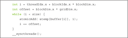
After zeroing the histogram, the next step is remarkably similar to our original GPU histogram. The sole differences here are that we use the shared memory buffer temp[] instead of the global memory buffer histo[] and that we need a subsequent call to __syncthreads() to ensure the last of our writes have been committed.
The last step in our modified histogram example requires that we merge each block’s temporary histogram into the global buffer histo[]. Suppose we split the input in half and two threads look at different halves and compute separate histograms. If thread A sees byte 0xFC 20 times in the input and thread B sees byte 0xFC 5 times, the byte 0xFC must have appeared 25 times in the input. Likewise, each bin of the final histogram is just the sum of the corresponding bin in thread A’s histogram and thread B’s histogram. This logic extends to any number of threads, so merging every block’s histogram into a single final histogram involves adding each entry in the block’s histogram to the corresponding entry in the final histogram. For all the reasons we’ve seen already, this needs to be done atomically:
Since we have decided to use 256 threads and have 256 histogram bins, each thread atomically adds a single bin to the final histogram’s total. If these numbers didn’t match, this phase would be more complicated. Note that we have no guarantees about what order the blocks add their values to the final histogram, but since integer addition is commutative, we will always get the same answer provided that the additions occur atomically.
And with this, our two phase histogram computation kernel is complete. Here it is from start to finish:

This version of our histogram example improves dramatically over the previous GPU version. Adding the shared memory component drops our running time on a GeForce GTX 285 to 0.057 seconds. Not only is this significantly better than the version that used global memory atomics only, but this beats our original CPU implementation by an order of magnitude (from 0.416 seconds to 0.057 seconds). This improvement represents greater than a sevenfold boost in speed over the CPU version. So despite the early setback in adapting the histogram to a GPU implementation, our version that uses both shared and global atomics should be considered a success.
9.5 Chapter Review
Although we have frequently spoken at length about how easy parallel programming can be with CUDA C, we have largely ignored some of the situations when massively parallel architectures such as the GPU can make our lives as programmers more difficult. Trying to cope with potentially tens of thousands of threads simultaneously modifying the same memory addresses is a common situation where a massively parallel machine can seem burdensome. Fortunately, we have hardware-supported atomic operations available to help ease this pain.
However, as you saw with the histogram computation, sometimes reliance on atomic operations introduces performance issues that can be resolved only by rethinking parts of the algorithm. In the histogram example, we moved to a two-stage algorithm that alleviated contention for global memory addresses. In general, this strategy of looking to lessen memory contention tends to work well, and you should keep it in mind when using atomics in your own applications.