
40 POTENTIAL PROBLEMS
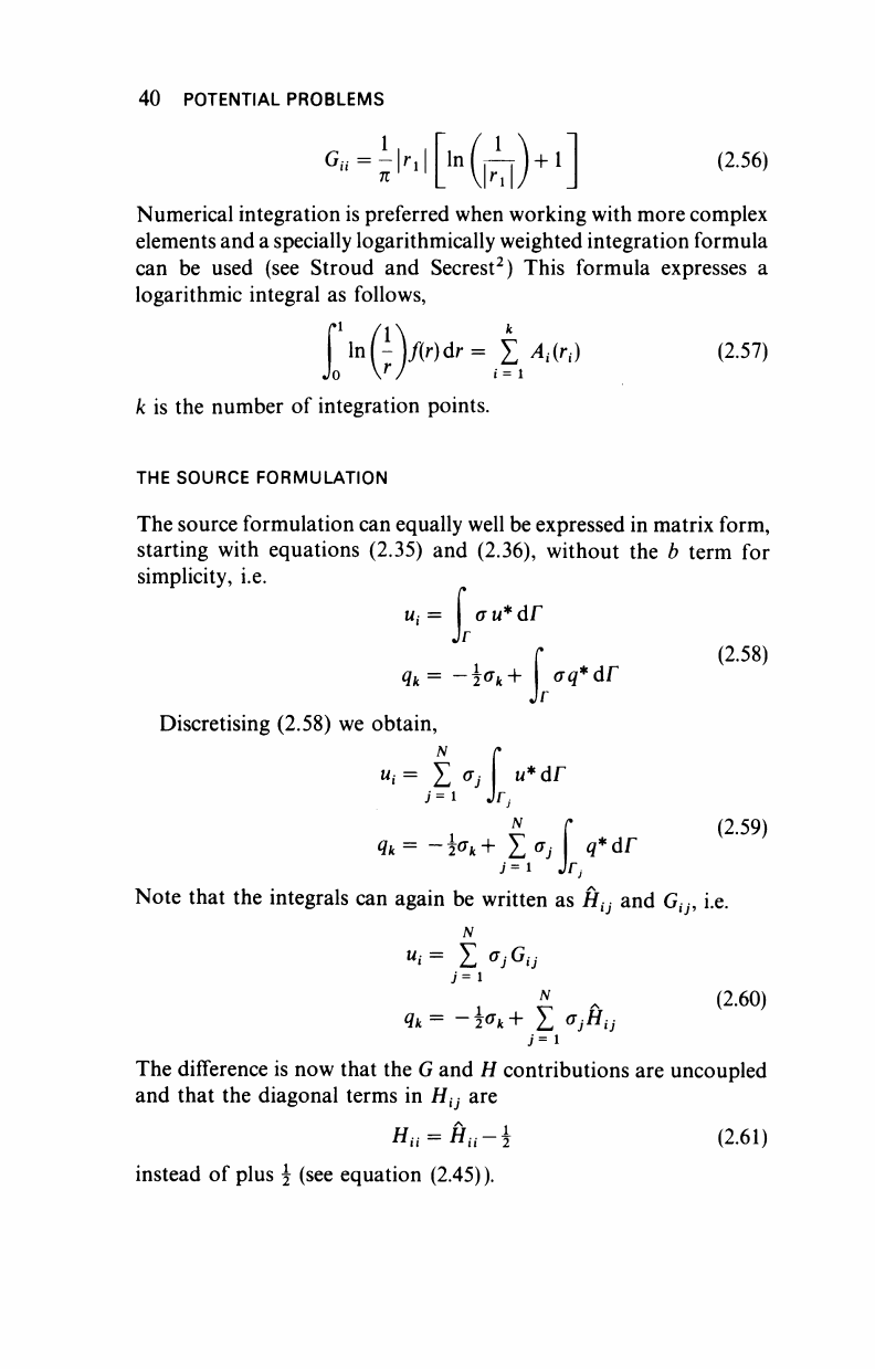
Ga
1
π
r
i 1
"ln(
' 1
J
r
i|
M
/ _
(2.56)
Numerical integration is preferred when working with more complex
elements and a specially logarithmically weighted integration formula
can be used (see Stroud and Secrest
2
) This formula expresses a
logarithmic integral as follows,
In
f(r)dr= Σ Mn)
(2.57)
k is the number of integration points.
THE SOURCE FORMULATION
The source formulation can equally well be expressed in matrix form,
starting with equations (2.35) and (2.36), without the b term for
simplicity, i.e.
au*dr
U; =
Ik
rq*dr
Discretising (2.58) we obtain,
N r
u
i
= Σ
σ
)
u
*
άΓ
j =
1
JTj
N r
j=i Jrj
(2.58)
(2.59)
Note that the integrals can again be written as H
i}
and
G
ij9
i.e.
".·= Σ <rjG
u
N
(2.60)
The difference is now that the G and H contributions are uncoupled
and that the diagonal terms in Η
{]
are
Η
Η
= Η
η
- (2.61)
instead of plus (see equation (2.45)).
POTENTIAL PROBLEMS 41
Formula (2.60) can now be written as,
N
".·= Σ °J
G
ij
N
(2.62)
<lk= L
a
j
H
kj
Equations (2.62) gives a system of 2N equations which can now be
reduced to a N x N system if the necessary boundary conditions are
applied,
Ui
= w, at N
i
points on Γ
χ
(2.63)
<lk
—
<lk
at
N
2
points on Γ
2
The final system can then be written as,
Ασ = F (2.64)
where the unknowns in the σ vector are the source intensities.
It is important to point out that an 'equilibrium' type requirement
should be introduced in two-dimensional problems. The reason is
that the potentials given by (2.62) are only relative potentials in two-
dimensional problems. This is because of the special logarithmic
character of the solution, i.e.
u*
= - (2π)~
ι
ln(l/r), which implies that
w* does not go to zero at infinity.
As the choice of datum is arbitrary we can write
",·= Σ efiij + C (2.65)
j=i
where C is an unknown constant. The system has now (iV + 1)
unknowns but we can solve it by adding the following 'equilibrium'
condition:
/»
σάΓ = 0 (2.66)
Jr
or in discrete form,
Σ
*^
= °
(
2
·
67
)
where /, is the length of each element. This equation represents the
requirement that the sum of all the sources applied is zero and will
42 POTENTIAL PROBLEMS
ensure that its effect at infinity
is
zero.
Another way of ensuring this is
by closing the domain with
a
series
of
boundary elements
far
away
from
the
body.
Example
2.2
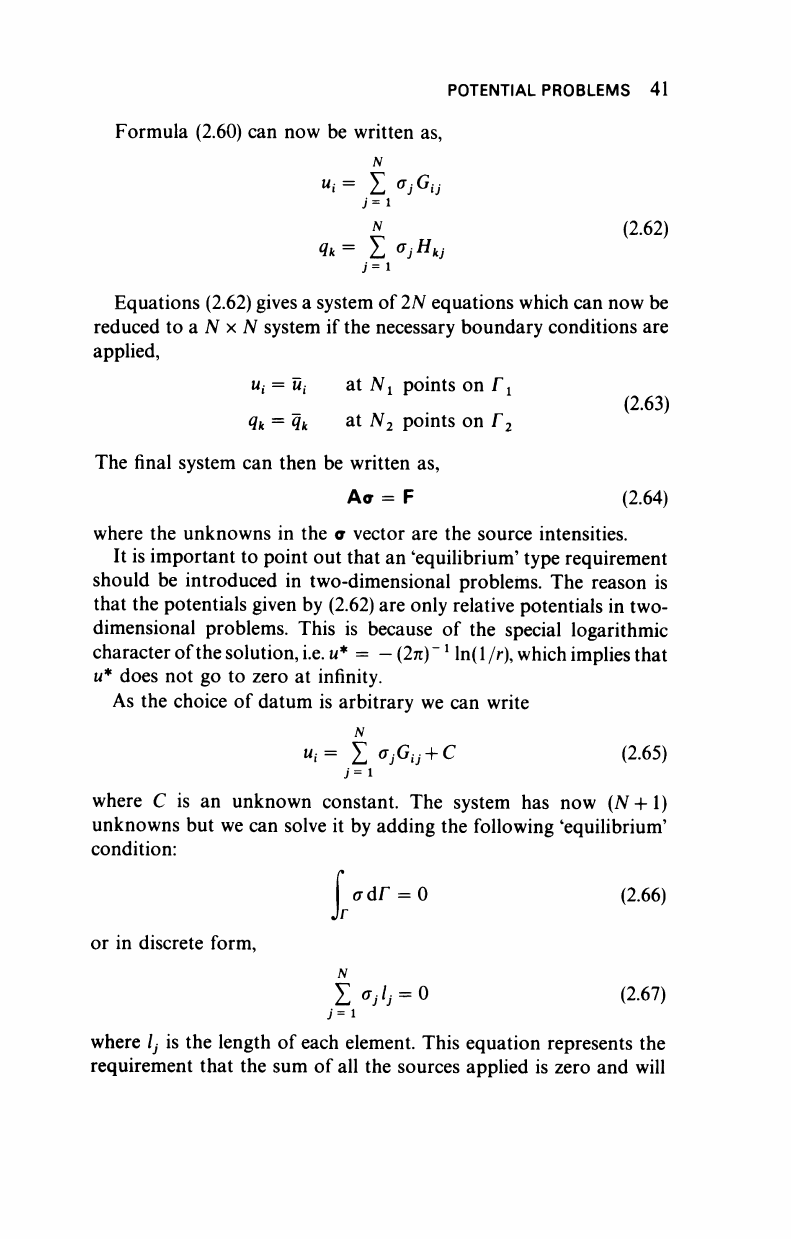
Figure 2.7 depicts the
first
application
of
finite
elements to fluid flow,
i.e.
a
flow around
a
cylinder between parallel plates,
and is due to
Martin.
3
u
represents the stream function and
du/dn
are the velocities
along
the
boundaries.
The
values
of the
stream function
and its
derivative
are
shown
in
Figure 2.7.
u=
2
/
\\\\\w\
du/dn=0
ΧΛ\\\\\\
27
26 25 2k 23 22 21 20
19
1817
28
29
30
31
32
-· 1
· i · i ·
3
A 5
2k
30 36 k2 48 54 60 66
72 nodes
110 elements
Figure
2.7 Flow
around
a cylinder
between
parallel plates. Constant boundary
elements
versus finite element grid

POTENTIAL PROBLEMS 43
Because of symmetry we need only to consider a quarter of the
domain. This has been discretised using 110 finite elements with 72
nodes.
A
constant boundary element grid with the same density on the
boundaries has only 32 elements or nodes. Figure
2.8(a)
shows the
prescribed u and du/dn values along the boundary and Figure
2.8(b)
the computed values for
u
and du/dn. Note that the variation of du/dn
velocities is the one expected.
28
29
K30
u
=
2
27 26 25 2k 23 22 21 20 19 18 17
• i · 1 · ■ · i ·—i · . · i · i ·
■
· . ·
16
415
tU
13
12
l ΊΊ
32
U
U—· 1—· ■ » ■ ·
u
=
0
3
c/=0
du/dn^O
(b)
du
Idn
J
£
^
du/dn
Figure
2.8
Prescribed
conditions and
solution for constant
elements,
(a)
Values
ofu
and
du/dn prescribed along boundary; (b) computed
values
for u and du/δη along boundary
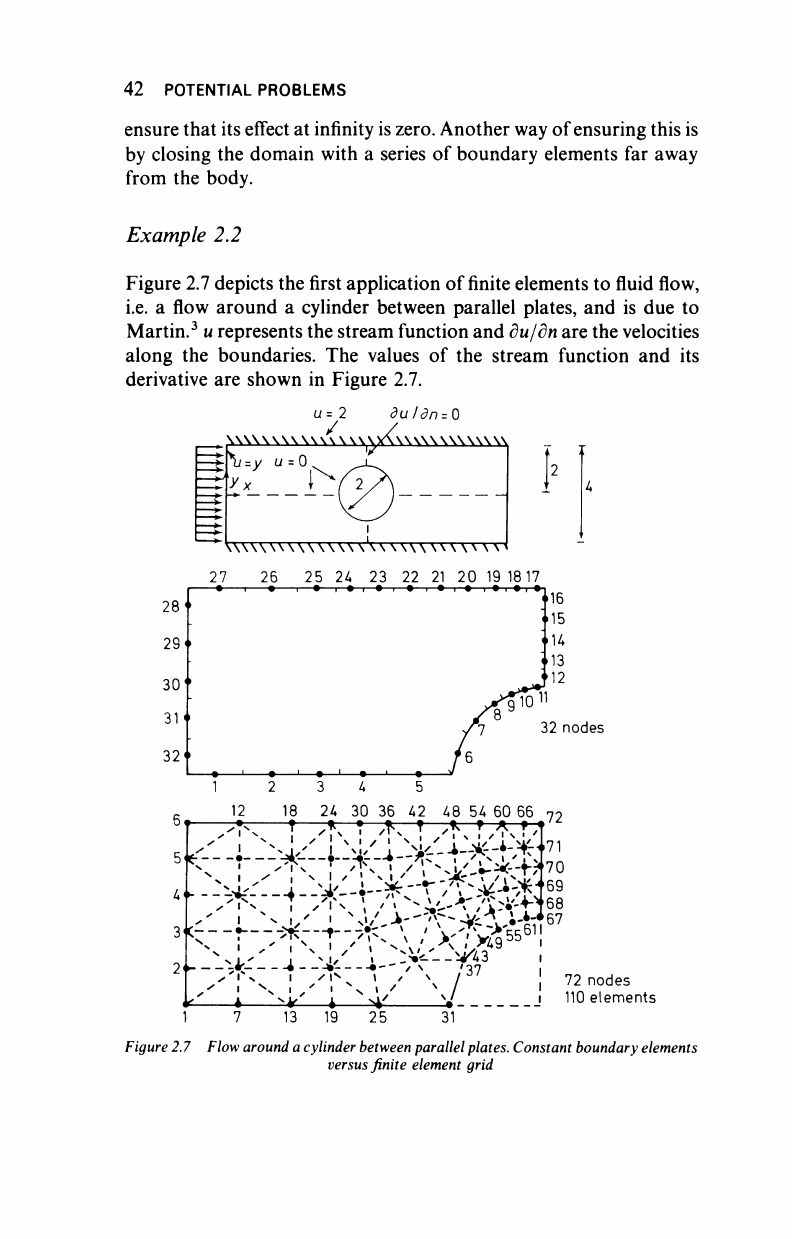
44 POTENTIAL PROBLEMS
Values of u inside the domain agree well with the finite elements
results and the cell collocation solution (developed in Lau and
Brebbia
4
). The cell collocation method for this case is similar to a
curvilinear finite difference technique.
u
=
2
12 18 24 30 36 42 48 54 60 66
—· ·
·—·—·
·—·—·—·—·—
'43
Γ37
55
c
72
71
70
69
68
67
du/dn
13 19 25
u
= Q
31
du/dn
J
du/dn
Figure 2.9 Prescribed conditions and
solution
for finite elements, (a) Values of
u
and
du/dn prescribed along boundary; (b) computed
values
for u and du/dn along boundary
Notice that the values of velocities (du/dn) calculated on the
boundaries using
finite
elements are unsatisfactory (Figure
2.9),
while
the boundary element and cell collocation solutions represent the
expected flow configuration well. A comparison of values of u for
..................Content has been hidden....................
You can't read the all page of ebook, please click here login for view all page.