3.9 The circular normal distribution

3.9.1 Distributions on the circle

In this section, the variable is an angle running from to , that is, from 0 to radians. Such variables occur in a number of contexts, for example in connection with the homing ability of birds and in various problems in astronomy and crystallography. Useful references for such problems are Mardia (1972), Mardia and Jupp (2001), and Batschelet (1981). The method used here is a naïve numerical integration technique; for a modern approach using Monte Carlo Markov Chain (MCMC) methods, see Damian and Walker (1999).

The only distribution for such angles which will be considered is the so-called circular normal or von Mises’ distribution. An angle is said to have such a distribution with mean direction μ and concentration parameter κ if

and when this is so we write

The function is the modified Bessel function of the first kind and order zero, but as far as we are concerned it may as well be regarded as defined by

It is tabulated in many standard tables, for example, British Association (1937) or Abramowitz and Stegun (1965, Section 9.7.1). It can be shown that

The circular normal distribution was originally introduced by von Mises (1918). It plays a prominent role in statistical inference on the circle and in that context its importance is almost the same as that of the normal distribution on the line. There is a relationship with the normal distribution, since as the distribution of

approaches the standard normal form N(0,  1) and hence is approximately . It follows that the concentration parameter is analogous to the precision of a normal distribution. This is related to the fact that asymptotically for large κ

However, the equivalent of the Central Limit Theorem does not result in convergence to the circular normal distribution. Further, the circular normal distribution is not in the exponential family. It should not be confused with the so-called wrapped normal distribution.

The likelihood of n observations from an distribution is

so that if we define

then (c, s) is sufficient for given , and indeed

If we define

then we get

and hence

(It may be worth noting that it can be shown by differentiating with respect to the that ρ is a maximum when all the observations are equal and that it then equals unity.) It is easy enough now to construct a family of conjugate priors, but for simplicity let us consider a reference prior

It seems reasonable enough to take a uniform prior in μ and to take independent priors for μ and κ, but it is not so clear that a uniform prior in κ is sensible. Schmitt (1969, Section 10.2) argues that a uniform prior in κ is a sensible compromise and notes that there are difficulties in using a prior proportional to since, unlike the precision of a normal variable, the concentration parameter of a circular normal distribution can actually equal zero. If this is taken as the prior, then of course

3.9.2 Example

Batschelet (1981, Example 4.3.1) quotes data on the time of day of major traffic accidents in a major city. In an obvious sense, the time of day can be regarded as a circular measure, and it is meaningful to ask what is the mean time of day at which accidents occur and how tightly clustered about this time these times are. Writing

the n = 21 observations are as follows:

This results in and and so (allowing for the signs of c and s) (or in terms of a time scale 16h 34m) and so the posterior density takes the form

where ρ and μ take these values. It is, however, difficult to understand what this means without experience of this distribution, and yet there is no simple way of finding HDRs. This, indeed, is one reason why a consideration of the circular normal distribution has been included, since it serves to emphasize that there are cases where it is difficult if not impossible to avoid numerical integration.

3.9.3 Construction of an HDR by numerical integration

By writing and taking the first few terms in the power series quoted earlier for , we see that for

to within 0.002. We can thus deduce some values for and , namely,

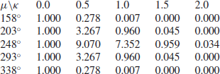
As n = 21, this implies that (ignoring the constant) the posterior density for , 0.5, 1.0, 1.5, and 2.0 and for values of μ at intervals from is

In order to say anything about the marginal density of μ, we need to integrate out κ. In order to do this, we can use Simpson’s Rule. Using this rule, the integral of a function between a and b can be approximated by the sum

where the xi are equally spaced with x0=a and x4=b. Applying it to the aforementioned figures, we can say that very roughly the density of μ is proportional to the following values:

Integrating over intervals of values of μ using the (even more crude) approximation

(and taking the densities below 158 and above 338 to be negligible) the probabilities that μ lies in intervals centred on various values are proportional to the values stated:

It follows that the probability that μ lies in the range (203, 293) is about 256/552=0.46, and thus this interval is close to being a 45% HDR.

3.9.4 Remarks

The main purpose of this section is to show in some detail, albeit with very crude numerical methods, how a Bayesian approach can deal with a problem which does not lead to a neat posterior distribution values of which are tabulated and readily available. In practice, if you need to approach such a problem, you would have to have recourse to numerical integration techniques on a computer, probably using MCMC as mentioned at the start of this section, but the basic ideas would be much the same.