CHAPTER 5

AI Solutions for Security

• Discovery Phase
• Detect Phase
• Threat Score Phase
• Threat Response Phase
• Protect Phase
• Monitor Phase
• Conclusion
• Firms in AI Cybersecurity

Chapter Outline

• How to handle AI/ML models for security solutions

Key Learning Points

• Learn and understand how AI/ML applies to security areas
• Data preparation for
  • Input
  • Output
  • Training data
  • Validation data
• Evaluate different algorithms

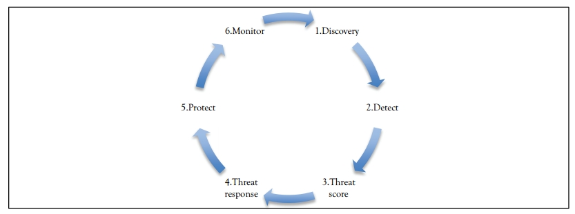
Figure 5.1 Security AI process

Security AI Process

The artificial intelligence (AI) system being developed uses the following design approach:

• Discovery phase
• Detect phase
• Threat score phase
• Threat response phase
• Protect phase
• Monitor phase

See Figure 5.1. The necessary process is shown here.

Discover Phase

• Assets
  • People
  • Process
  • Things and objects
  • Technology
  • Event
  • Action
• Data
  • Logs
  • System and server
  • Network activity
  • Host
  • Firewall
• Threats
  • Entry point, end point, and edge
  • Breaking to the system, host, and firewall
  • Vulnerable assets
• Intrusion and violation
  • Possible violation of assets

Detect Phase

• Signature-based detection (recognizing bad patterns such as malware).
• Anomaly-based detection [detecting deviations from a model of “good” traffic, which often relies on machine learning (ML)].

Threat Score

• Scoring the identified or detected threats.

Threat Response

• Identifying the best possible actions to be taken against the high-score threats.

Protect

• Take automatic actions or manual actions from the threat response phase.
• Example actions: block the IP, disable the user, or block all the access in the firewall.

Monitor

• Monitoring actions
• How often?
  • Mostly real time
• Monitoring assets
  • Monitoring people
  • Monitoring processes
  • Monitoring things and objects
  • Monitoring technology
  • Monitoring events
  • Monitoring actions
  • Monitoring data
  • Monitoring threats
  • Monitoring intrusions and violations
• Monitoring output
• Dashboard
• Score card
• Alerts (how critical the issue is)

This process helps companies address vulnerabilities and neutralize threats proactively instead of waiting for hackers to exploit high-security vulnerabilities.

The following sections will go through the AI process in detail.

Discover AI

Define Goal

• What assets pose serious threats?
• What assets are vulnerable?

Data Collection

Input:

• Table 5.1 illustrates sample assets in the organization.
• Table 5.2 illustrates network traffic connection logs, network metadata, and flow data (conversation between two hosts).
• Table 5.3 illustrates network metadata extracted features.
• Network metadata additional extracted features:
  • These features can help the machine detect zero-day (before the actual attack happens) and web application attacks. See Table 5.4.
• Network metadata shellcode extracted features (advanced):
  • In hacking, a shellcode is a small piece of code used as the payload in the exploitation of a software vulnerability.
  • Extracted features are useful for detecting shellcode and malware. The shellcode is a bundle of codes or scripts that look like valid script. Shellcode typically starts as a command shell from which the attacker can control the compromised machine; however, any piece of code that performs a similar task can be called shellcode.
    See Table 5.5.
• Table 5.6 illustrates security events.
• List of software with vulnerabilities:
  • Product, software, vendor, number of entries, software type, vulnerabilities, patches, compliance, and inventory.
• More features can be extracted using Natural Language Processing (NLP) techniques from structured and unstructured sources such as blog feeds, twitter feeds, and news feeds.

Output (label):

• Possibility of vulnerability
• Value: true or false

Table 5.1 Assets in the organization

Device	IP Address	Type	Model
MacbookPro	192.168.2.100	Apple Mac	Apple MacBook Pro 2013
JohnDesktop	192.168.2.101	Computer	Windows XP
First Floor	192.168.2.102	Printer	HP Officejet 4650
Conference Room 1	192.168.2.103	Router	Netgear Nighthawk R7000

Table 5.2 Network traffic log

Event Time	Connection ID	Source IP/Port	Dest IP/Port	Data Transferred (bytes)	Bytes Uploaded (bytes)	Bytes Downloaded (bytes)	Flow Duration (sec)
Thu Sep 24 09:00	123123132	192.168.2. 100: 4700	192.168.2.101: 80	23423423	2342234234	32423434	1029

Table 5.3 Network metadata extracted features

Event Time	Connection ID	No. of Security Keywords	Min. Byte Value	Max. Byte Value	No. of Distinct Bytes	No. of Nonprint Chars	No. of Punctuation Chars
Thu Sep 24 09:00	123123132	3	4	9	100	3	5

Table 5.4 Network metadata additional extracted features

Event Time	Connection ID	Contains Shell Code	Contains JavaScript Code	Contains SQL Command	Contains Command Injection
Thu Sep 24 09:00	123123132	Y	N	N	N

Table 5.5 Network metadata shellcode extracted features

Event Time	Connection ID	API Call Sequence
Thu Sep 24 09:00	123123132	1
Thu Sep 24 09:15	123123132	2

Table 5.6 Security events

Event Time	Event	Description	I/S	Source IP
Thu Sep 24 09:00	SV1	Local logon success	S	192.168.2.100
Thu Sep 24 09:15	SV2	Local logon fail	I	192.168.2.101
Thu Sep 24 09:15	SV3	Network traffic overload	I	192.168.2.101
Thu Sep 24 09:15	SV4	CPU usage overload	I	192.168.2.101
Thu Sep 24 09:15	SV5	Disk usage overload	I	192.168.2.101

ML/AI use case:

This is a binary classification problem for list of all assets.

Design Algorithm

Binary classifiers can be used for this model.

Identify Features

From the above datasets, 11 of the most important and generic features are selected out of all features to train ML and AI models to recognize the vulnerable assets.

• Source IP
• Date
• Timestamp
• Time zone
• IP location
• Number of TCP/IP requests
• Number of requests with nonprintable characters
• Number of requests with punctuation characters
• Number of requests containing JavaScript
• Number of requests containing Structured Query Language (SQL) statement
• Number of requests containing command injection
• Number of API call sequences
• Number of failed security events
• Number of successful security events
• Number of vulnerable software installed
• Vulnerable (label and output)

Train the Model

Train the selected algorithms using the prepared dataset.

Tuning the hyperparameters to train the model.

Run the training multiple times with different combinations of the provided hyperparameters of batch size, epochs, optimizer, learn rate, momentum, and dropout rate to find the optimum combination of hyperparameters to determine the appropriate results.

• Batch size = [10, 20, 40, 60, 80, 100]
• epochs = [10, 50, 100]
• optimizer = [‘SGD’, ‘RMSprop’, ‘Adagrad’, ‘Adadelta’, ‘Adam’, ‘Adamax’, ‘Nadam’]
• learn rate = [0.001, 0.01, 0.1, 0.2, 0.3]
• momentum = [0.0, 0.2, 0.4, 0.6, 0.8, 0.9]
• dropout rate = [0.0, 0.1, 0.2, 0.3, 0.4, 0.5, 0.6, 0.7, 0.8, 0.9]

It is recommended to try out different combinations of hyperparameters using grid search.

Grid search = GridSearchCV(estimator=model, param_grid=param_grid, n_jobs=−1, scoring=’accuracy’)

Compare models with different hyperparameters and choose the best fit. Use the model to train further using the full dataset.

Test the Model

Test the model using the test dataset for each selected algorithm with given methods:

• Specify the used loss function with respective algorithms
• Learning rate curve
• Learning curve

See Figure 5.2. Pick the model with the “Learning rate- Good,” depicted in the graph.

Figure 5.2 Loss versus epoch learning graph

Receiver Operating Characteristic Curve

Receiver operating characteristic curve is another common tool used with binary classifiers. See Figure 5.3. For this use case, let’s choose the model with false positive rate of 0.99, since 90 percent accuracy is expected from Discover AI Model.

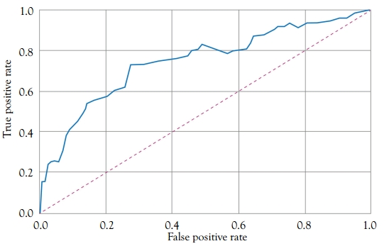
Figure 5.3 ROC curve

Evaluate the Model

Evaluate the model using accuracy and the mean square error (MSE) to determine the learning rate. The following scoring methods are
used.

Scoring Methods

• Precision score
• Recall score
• F1 score
• Support score
• Accuracy score
• Area under the curve/receiver operating characteristic curve
• Learning rate (ranges from 0 to 1)

Confusion Matrix

• Analyze the inputs that are improperly classified using the confusion matrix.
• Note the accuracy versus epoch graph.
• Decide the final model with accuracy.

Repeat the steps from data collection, data preparation, feature extraction, training, testing, and evaluation of the model until the necessary accuracy of 85 and above is reached.

Table 5.7 shows the classification accuracy output obtained using several ML algorithms.

Table 5.7 Classification algorithm and accuracy

Naïve Bayer	81.5%
SVM	88.5%
J48	91%
Bayesian network	94%
Multinomial logistic regression	96.5%
FT (classifier for building “Functional Tree,” classification trees that could have logistic regression functions at the inner nodes)	99.5%
SMO (implements John Platt’s sequential minimal optimization algorithm for training a support vector classifier)	99.8%
Multilayer perceptron	100%

Model Conclusion

Based on the classification accuracy, multilayer perceptron is the best performing model for this binary classification problem.

Publish and Production of the Model

• Retrain the model until the desired output is reached.
  • Repeat the steps from data collection, data preparation, feature extraction, training, testing, and evaluation, and then publish the model.
  • Repeat the whole process for all the measures in this business process as explained in the evaluation steps.
• Here are the possible ways to produce the trained model:
  • Host in Google Cloud, Microsoft Azure, or Amazon Web Services (AWS).
• How to deploy the trained model:
  • https://Cloud.google.com/ml-engine/docs/tensorflow/deploying-models
• Regularly monitor and update the model.
• How to use the produced model for businesses:
  • Integrate the trained model with the application so businesses can identify new securities or threats using the new dataset.

Conclusion

Type of resources needed for this project are as follows:

• Security threats analysis and subject matter expert
• Security threats mitigation strategists
• Data analysts
• Data architects
• Data scientists
• Data engineers

To simplify all the above steps, check out www.BizStats.AI

The automated steps are as follows:

• Provide input dataset
• Train multiple models
• Presented models with accuracy
• Pick and activate the model
• Use the model through a direct search.

Detect AI

Define Goal

Step 1: Detect the threats that have happened, are happening, or are going to happen

Step 2: Categorize the threat

• Categories
  • User threat (phishing, ransomware)
  • Application threat (cross-site scripting and SQL injection)
  • Infrastructure threat (botnet, Trojan-DDoS)
  • Operations risks
  • Hardware risks
  • Software risks
  • Project risks
  • Personnel risks
  • Data risks
  • Vendor risks
  • Disaster and business continuity risks
  • Compliance and security risks

Data Collection

Input the following (Table 5.8):

• Data from previous step.
• Vulnerable assets data from previous steps.
• Browser events (identification, date, user, PC, uniformed resource locator (URL), activity, and content).
• User security events [identification, date, user, PC, and activity (log on and logoff information)].
• Device events (identification, date, user, PC, file, tree, and activity).
• E-mail events (identification, date, user, PC, recipients, activity, size, attachments, and content).
• File events (identification, date, user, PC, filename, activity, to removable, from removable, and content).
• Decoy files (file name and PC).
• Employees list: (user first name and last name).
• Threat intelligence data (campaigns and attack patterns).
• File (dynamic link library and executable), static features [amount of byte randomness (entropy) in the text section, the number of sections, and the presence or absence of particular API calls].
• File dynamic features extracted by running it in the sandbox [central processing unit use (percentage), random access memory use (count), swap memory use (count), received packets (count), received bytes (count), sent packets (count), sent bytes (count), and number of processes running (count)].

Table 5.8 Malwa attack data

Phishing URL	Targeted Brand	Time (UTC)
http://some…site.url/https.bb.de.jb/index1.html	Generic/Spear Phishing	17:43:24
http://some…site.url/https.bb.de.jb/index2.html	Generic/Spear Phishing	17:47:24
http://some…site.url/https.bb.de.jb	Generic/Spear Phishing	17:43:24

Output:

• Step 1
  • Is it a threat or not?
  • Values: yes or no
• Step 2
  • What type of threat is this?
  • Possible values: user threat, application threat, and infrastructure threat.
• ML and AI use case:
• Step 1
  • It is a binary classification problem?
• Step 2
  • This is a multiclass classification problem.

Design Algorithm

• Step 1
  • Binary classifiers can be used for this model.
• Step 2
  • Multiclass classifiers can be used for this model.

Identify Features

From the input datasets, the following features have been selected for this model:

Step 1: Detect the threat.

See Table 5.9.

Table 5.9 Detect the threat data sample

ID	Date	User	PC (mac address)	Event Type	Acti-vity	From	To	Size	Attach-ments	Con-tent	Threat
12w21	Thu Sep 24 09:00	john	sdf-dfdf-df-dfd-fd	E-mail	Sent	User	To, cc, bcc	10 MB	Yes	E-mail body	Y
w12d2	Thu Sep 24 09:00	smith	sdf-dfdf-df-dfd-fd	File	Download	External device	Dest IP/PC	100 MB	No	File content	Y
wewd23	Thu Sep 24 09:00	chris	sdf-dfdf-df-dfd-fd	Browser	Http visit	URL	Dest IP/PC	2 MB	No	Page content	N
2dgfg34	Thu Sep 24 09:00	jennifer	sdf-dfdf-df-dfd-fd	User Security	Logon	-	Dest IP/PC	-	No	-	N
32rffedc	Thu Sep 24 09:00	jack	sdf-dfdf-df-dfd-fd	Device	Connected	External	Dest IP/PC	10 GB	No	File tree	Y

Step 2: Categorize the threat. Only the threats are passed to this step.

See Table 5.10.

Table 5.10 Categorize the threat data sample

ID

Date

User

PC (mac address)

Event Type

Acti vity

From

To

Size

Attach ments

Content

Threat

Threat Category

12w21

Thu Sep 24 09:00

john

sdf-dfdf-df-dfd-fd

E-mail

Sent

User

To, cc, bcc

10 MB

Yes

E-mail body

Y

Insider threat

w12d2

Thu Sep 24 09:00

smith

sdf-dfdf-df-dfd-fd

Network

Files received

URL

Dest IP/PC

100 MB

No

File content

Y

Application threat

32rffedc

Thu Sep 24 09:00

jack

sdf-dfdf-df-dfd-fd

Device

Connected

External

Dest IP/PC

10 GB

No

File tree

Y

User threat

Identify List of Algorithms

• Binary classification algorithms.
• Multiclass classification algorithms.
• Deep learning with unsupervised learning.
• Clustering
  • Generally, this refers to the segregation of data into groups that have similar traits for the purpose of deciding a set of associated actions related to that grouping.
  • Clustering may be helpful in identifying security data from similar attack patterns by actors.
• Anomaly detection
  • This is especially useful for identifying “unknown unknowns” such as zero-day threats.

Train the Model

Step 1: Detect the threat

This step is the same as the “Discover AI” step.

Step 2: Categorize the threat

Use the identified datasets to train the model.

• Split the dataset into three sets as illustrated below:
  • Training dataset (60 percent)
  • Test dataset (20 percent)
  • Validation dataset (20 percent)
• Tune the hyperparameters to train the model as done to
  Discover AI models.
• Train the model for multiple iterations with 100 epochs per iteration.
• Train the model for various combinations of features to find the best model.

Tune the Model

Tune the hyperparameters to train the model.

Run the training multiple times with different combinations of the hyperparameters of selected algorithms. This typically includes batch size, epochs, optimizer, learn rate, momentum, and dropout rate to find the optimum combination of hyperparameters to determine the appropriate results.

Compare models with different hyperparameters and choose the best fit. Then, use the model to train using the full dataset.

Test the Model

Step 1 is the same as the “Discover AI” step.

Step 2 is the same as the “Discover AI” step, except it uses a multiclass classification.

Evaluate the Model

Step 1 is the same as the “Discover AI” step.

Step 2: Categorize the threat

Evaluate the model using accuracy, MSE, and determine the learning rate.

Use Confusion Matrix

Confusion matrix measures the performance of the classification algorithms. See Figure 5.4.

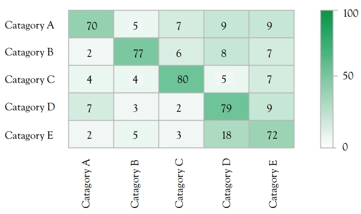
Figure 5.4 Confusion matrix predicted versus targeted

Confusion matrix graph for multiclass classification:

• X: Predicted value [security categories], 5 (1 to 5).
• Y: Targeted value [target categories], 5 (1 to 5).

Use encoded values instead of actual security categories.

Precision–Recall Curves

Precision–recall curves measure the success of the classification model.

See Figure 5.5.

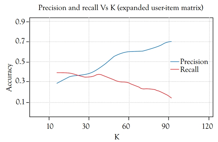
Figure 5.5 Precision and recall versus K

Check mistakes of the classification model on each label and analyze to fine-tune (see Figure 5.6).

Figure 5.6 Accuracy versus epoch graph

Decide the final model with accuracy

• If the classification prediction is wrong, you can improve the accuracy by using more training data. Therefore, collect more data then retrain the classification and reevaluate the model for the improvement on the accuracy.
• If the case is “classification prediction is wrong because of wrong training data,” use urAI-text annotation tool (https://bizstats.ai/product/urAI.html) to correct the input training data, then retrain the classification and reevaluate the model for the improvement on the accuracy.
  • Another method of evaluating the model accuracy is to use ensemble learning methods.

The ensemble learning methods are as follows:

• Sequential ensemble methods.
• Parallel ensemble methods.
• Combination of both.
• Weighted majority rule ensemble classifier.

Based on our experiments, the finalized ensemble classifier method is “weighted majority rule ensemble classifier.” This provides better accuracy than any other ensemble methods.

Weighted Majority Rule Ensemble Classifier

Three different classification models can be used to classify the samples: logistic regression, a naive Bayes classifier with a Gaussian kernel, and a random forest classifier all combined into an ensemble method.

• Cross-validation (five-fold cross-validation) results provide the following:
  • Accuracy: 0.90 (±0.05) [logistic regression].
  • Accuracy: 0.92 (±0.05) [random forest].
  • Accuracy: 0.91 (±0.04) [naïve Bayes].

The cross-validation results show that the performance of the three models is almost equal.

A simple ensemble classifier class can be implemented to combine the three different classifiers. A predict method simply takes the majority rule of the predictions by the classifiers. Here are some examples:

• Classifier 1 to class 1.
• Classifier 2 to class 1.
• Classifier 3 to class 2.

Now, classify the sample as “class 1.”

Furthermore, adding a weights parameter assigns a specific weight to each classifier. To work with the weights, collect the predicted class probabilities for each classifier, multiply it by the classifier weight, and take the average based on these weighted average probabilities. Next, one must assign the class label.

To illustrate this with a simple example, let us assume to have three classifiers and three-class classification problems to assign equal weights to all classifiers (the default): w1 = 1, w2 = 1, w3 = 1.

The weighted average probabilities for a sample would be calculated as follows (see Table 5.11).

Table 5.11 Weighted average calculation

Classifier Name	Class 1	Class 2	Class 3
Classifier 1	W1 * 0.2	W1 * 0.5	W1 * 0.3
Classifier 2	W1 * 0.6	W1 * 0.3	W1 * 0.1
Classifier 3	W1 * 0.3	W1 * 0.4	W1 * 0.3
Weighted average	0.37	0.4	0.3

The class 2 has the highest weighted average probability; thus, the sample is classified as class 2.

• Accuracy: 0.90 (±0.05) [logistic regression].
• Accuracy: 0.92 (±0.05) [random forest].
• Accuracy: 0.91 (±0.04) [naive Bayes].
• Accuracy: 0.95 (±0.03) [ensemble].

The ensemble classifier class is used to apply to majority voting using the class labels if no weights are provided and the predicted probability values show otherwise (see Table 5.12).

Table 5.12 Prediction based on majority class label

Classifier Name	Class 1	Class 2
Classifier 1	1	0
Classifier 1	0	1
Classifier 1	0	1
Prediction	-	1

Prediction based on predicted probabilities:

This is for equal weights: weights = [1, 1, 1]. See Table 5.13.

Table 5.13 Weighted average with prediction

Classifier	Class 1	Class 2
Classifier 1	0.99	0.01
Classifier 2	0.49	0.51
Classifier 3	0.49	0.51
Weighted average	0.66	0.18
Prediction	1	-

The results are different depending on whether a majority vote based on the class labels or the average of the predicted probabilities is applied. In general, it makes more sense to use the predicted probabilities (scenario 2). Here, “very confident” classifier 1 overrules the very unconfident classifiers 2 and 3.

A naive brute-force approach should be used to find the optimal weights for each classifier to increase the prediction accuracy.

The results look nice when applying the ensemble classifier (see Table 5.14). One must keep in mind that this is just a toy example. The majority rule voting approach might not always work so well in practice, especially if the ensemble consists of more “weak” than “strong” classification models. This uses a cross-validation approach to overcome the overfitting challenge, please always keep a spare validation dataset to evaluate the results.

Table 5.14 Example of compare table

Iteration	W1	W2	W3	Mean	Standard Deviation
2	1	2	2	0.953333	0.033993
17	3	1	2	0.953333	0.033993
20	3	2	2	0.946667	0.045216

Model Conclusion

Step 1 is the same as the “Discover AI” step.

Step 2: Categorize the threat.

Based on our experiment, the “weighted majority rule ensemble classifier” performs better than other algorithms for the “Detect AI: Categorize the threat model.”

Publishing and Production of Models

Step 1 is the same as the “Discover AI” step.

Step 2 is the same as the “Discover AI” step.

Conclusion

Step 1 is the same as the “Discover AI” step.

Step 2 is the same as the “Discover AI” step.

Threat Score AI

Define Goal

Score the identified threats for prioritization of issues for further investigation.

Data Collection

Input:

• Identified threats from step “Detect AI.”
• List of historical threats and their impact.
• External security events data.
• Blogs, articles, and news to understand the threat and its impact.

Output:

• Threat score (1–10).
• Continuous output variable.

ML and AI use case:

This is a regression problem.

Design Algorithm

Regression algorithms can be used for this model.

Identify Features

See Table 5.15.

Table 5.15 Threat score data sample

Event ID	Threat Type	Threat Impact (in dollars)	Likelihood of Exploi-tation (%)	Number of Social Media Shares	Level of Inter-connected-ness With Other Assets (%)	Does it Impact Critical Business Operation?	Size of User Base	Threat Score
wewd23	Hacking	5M	20	3k	20	Y	500	5
12w21	Data theft	24M	10	10k	15	Y	5M	8
w12d2	Cross-site scripting	2M	50	4k	25	N	100	3

Train the Model

Using Deep Neural Network Architecture

The deep neural network can be trained to predict the threat score (see Figure 5.7).

Figure 5.7 Fully connected neural network layer for deep neural networks

Fully connected neural network layers consist of a list of inputs into a list of outputs. Three basic types of layers exist: input layers, output layers, and hidden layers. The functionality-based layers are convolution layers, maximum and average pooling layers, dropout layer, nonlinearity layer, loss function layers, and much more (see Figure 5.8).

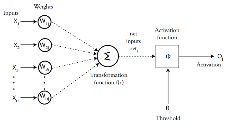
Figure 5.8 Activation function of neural network

This deep neural network consists of

• One input layer with 14 nodes.
• Three hidden layers with 256 nodes each with a ReLU activation function and a normal initializer, such as the kernel initializer.
• Mean absolute error as a loss function.
• Output layer with only one node.
• Use “linear” as the activation function for the output
  layer.

See Table 5.16.

Table 5.16 Deep neural network layers

Layer (type)	Output Shape	Param #
Input layer (Dense)	(none, 128)	19,200
Hidden layer 1 (Dense)	(none, 256)	33,024
Hidden layer 1 (Dense)	(none, 256)	65,792
Hidden layer 1 (Dense)	(none, 256)	65,792
Output layer (Dense)	(none, 1)	257
Total params: 184,065; trainable params: 184,065; non-trainable params: 0.

The validation loss of the best model is 18520.23 (see Figure 5.9).

Figure 5.9 Training log output

Using Other Algorithms

Use the identified datasets to train the model.

Fit a model using linear regression first and then determine whether the linear model provides an adequate fit by checking the residual plots. If a good fit cannot be obtained using linear regression, try a nonlinear model because it can fit a wider variety of curves. It is recommended to use ordinary least squares (OLS) first because OLS is easier to perform and interpret.

Use Akaike’s information criterion (AIC), Bayesian information criterion (BIC) (see Figure 5.10), or Mallows’ CP to decide how many factors should be used. These methods are better than comparing with R2.

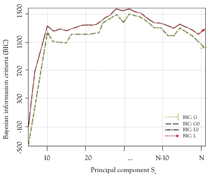
Figure 5.10 Principal components versus Bayesian information criterion

Use multiple regression. If the sample size is large enough, you may use autoselect option such as forward backward or best. This option will select independent factors using sampling techniques.

Test the Model

Test the model using the test dataset and expert knowledge.

Analyzing different metrics like statistical significance of parameters, R-square, adjusted r-square, and AIC, model is considered to be more likely to be the true model (BIC) and error term. Another one is the Mallow’s Cp criterion. This checks for possible bias in your model by comparing the model with all possible submodels (or a careful selection of them). See Figure 5.11.

The model is more accurate for the left graph.

You should not choose automatic model selection methods if your dataset has multiple confounding variables because you do not want to put these in a model at the same time. Regression regularization methods work well in case of high dimensionality and multicollinearity among the variables in the dataset.

Figure 5.11 R-squared comparison graph

Evaluate the Model

Evaluate the model using accuracy and MSE to determine the learning rate. Cross-validation is the best way to evaluate models used for prediction. Cross-validation divides your dataset into two groups (train and validate). A simple mean squared difference between the observed and predicted values gives you a measure for the prediction accuracy. See Figure 5.12.

Predicting threat score model using linear model:

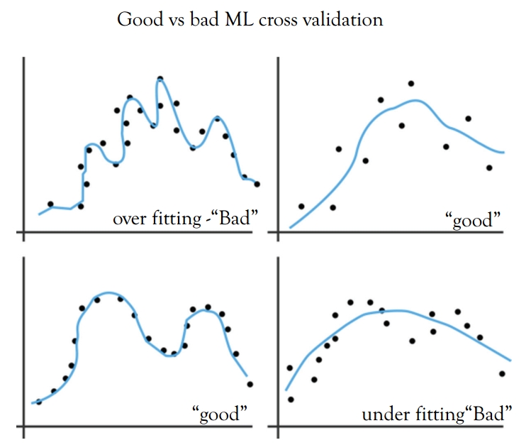
Figure 5.12 Cross-validation comparison

See Figure 5.13 for the predicted versus the actual and root mean square error (RMSE) score below.

Figure 5.13 Evaluate ensemble model predicted versus actual

Test RMSE score: 5.125877.

The threat score model is predicted using a bagged model. The bagged model is fitted using the randomForest algorithm. Bagging is a special case of a random forest where mtry (number of variables randomly sampled as candidates at each split) is equal to p, the number of predictors. Try using 13 predictors. Test RMSE score: 3.843966.

The model provides two interesting results. First, the predicted versus the actual plot no longer has a small number of predicted values. Second, our test error has dropped dramatically. Also note that the “mean of squared residuals,” which is output by randomForest, is the out of bag estimate of the error. For regression, the suggestion is to use mtry equal to p/3 = 4 predictors. Test RMSE score: 3.701805.

Here note the three RMSEs: the training RMSE (which is optimistic), the out-of-bag (OOB) RMSE (which is a reasonable estimate of the test error), and the test RMSE. Also note that the variables’ importance was calculated. See Table 5.17.

Table 5.17 Data versus error comparison

No	Data	Error
1	Training Data	1.558111
2	OOB	3.576229
3	Test	3.701805

Lastly, try using a boosted model. This model produces a nice variable importance plot and plots the marginal effects of the predictors. Based on this analysis, decide which variables most influence the threat score. See Table 5.18.

Table 5.18 Test error score of each model

	Model	Test Error
1	Single Tree	5.45808
2	Linear Model	5.12587
3	Bagging	3.84396
4	Random Forest	3.70180
5	Boosting	3.43382

Model Conclusion

Ensemble boosting model performed better than other algorithms for predicting threat score models.

Publishing and Production of Model

This is the same as the “Discover AI” step.

Conclusion

The same ML and AI model can be used for scoring the skills mentioned below.

Skills AI scoring models:

1. Respectfulness score (helping others retain their autonomy)
2. Courteousness score
3. Friendliness score
4. Kindness score
5. Honesty score
6. Trustworthy score
7. Loyalty score
8. Ethical score

The skills scoring models can be used with customers, customer support executives, project resources, vendors, suppliers, buyers, and much more.

Threat Response AI

Define Goal

Predict what response needs to be taken to fix the threat.

Data Collection

Input:

• Identify threats using the score from Discover AI, Detect AI, and Threat Score AI.
• Other inputs from Discover AI, Detect AI, and Threat Score AI.
  • Categories of threat
    • Human threats: Malicious human activity can be a major threat to your computer. For example, a discontented employee may try to tamper with or destroy data on an employer’s computer. A hacker is someone who tries to access your computer illegally via the Internet.
    • Processes
    • Things and objects
    • Technologies
    • Events
    • Actions
• List of historical threat responses and their impact.

Output:

• Predict what action needs to be taken toward the present threat.
• Values
  • Block
    • Determine whether there is a need to respond to the source of the event (e.g., blocking the source).
  • Deceive
    • Determine whether there is a need to respond in a manner that causes further action and events (e.g., modifying the response to the source so that it can learn more about the threats behavior).
  • Apply fix
    • Determine whether there is a need to fix the issues of the event (e.g., applying patch for the operating system).
  • No action
    • Determine whether there is a need to consider action at all (e.g., determine if the event is relevant to the environment or if it should remain unknown that the source has been detected).

ML and AI Use case:

This is a multiclass classification problem

Design Algorithm

This is the same as the “Detect AI: Categorize the threat” step.

Identify Features

This is the same as the “Detect AI: Categorize the threat” step.

Train the Model

This is the same as the “Detect AI: Categorize the threat” step.

Test the Model

This is the same as the “Detect AI: Categorize the threat” step.

Evaluate the Model

This is the same as the “Detect AI: Categorize the threat” step.

Model Conclusion

This is the same as the “Detect AI: Categorize the threat” step.

Publish/Production of Model

This is the same as the “Detect AI: Categorize the threat” step.

Conclusion

This is the same as the “Detect AI: Categorize the threat” step.

Protect AI

Define Goals

• Stop anomalous activity in real time: at the point of access.
• Take action automatically or notify users based on the threat response and AI output.

Data Collection

Input:

• Output of step “Threat Response AI.”
• List of historical protected and unprotected logs.
• Knowledge about previous protection steps.
• Protection rules.

Output:

• Action report.
• Automated steps needed to protect.
• If it is manual, provide the instruction steps needed to protect.
• Suggested action.
• Block the asset (e.g., remove the vulnerable desktop from network using mac address).
• Block the user (e.g., disable the user from logging into the network using username or other identification).

Design Algorithm

The following algorithms can be used for this model:

• Decision tree
• Reinforcement learning

Identify Features

Prepare data from the available input dataset and from the “Threat Response AI” step.

Train the Model

This is the same as the “Detect AI: Categorize the threat” step.

Test the Model

This is the same as the “Detect AI: Categorize the threat” step.

Evaluate the Model

This is the same as the “Detect AI: Categorize the threat” step.

Model Conclusion

This is the same as the “Detect AI: Categorize the threat” step.

Publish/Production of Model

This is the same as the “Detect AI: Categorize the threat” step.

Conclusion

This is the same as the “Detect AI: Categorize the threat” step.

Monitor AI

Define Goals

• Security monitoring:
  • Constantly monitors the security level of your assets, users, and external IPS to identify your greatest threats. Reviews historical alerts using probabilistic models to identify assets and uncovers deeper links between alerts and existing rules-based systems.
• Network threat detection technology:
  • Understands traffic patterns on the network and monitors traffic in and between trusted networks, as well as Internet traffic.
• Recover:
  • Continuously monitors and learns from the data it collects from various data. Recovery can provide a user-role assignment recommendation based on the least privileged model.
• Detect
  • Continuously monitors the near real-time event stream and detects anomalous behavior and potential threats with a threat detection engine. This engine uses big data analytics and real-time ML algorithms to automatically identify the risks from massive amounts of access event data and access entitlements data. Risky events are annotated with security scores as well as the security distribution and alerts are created.

Monitor in Discover Phase

This is done using dashboards and scorecards.

Monitor in Detect Phase

This is done using dashboards and scorecards.

Monitor in Threat Scoring Phase

This is done using dashboards and scorecards.

Monitor in Threat Response Phase

This is done using dashboards and scorecards.

Monitor in Protect Phase

This is done using dashboards and scorecards.

Firms in AI Cybersecurity

The development of AI techniques has seen AI appear in a lot of different IT products, including the field of cybersecurity. Here are some key innovators in cybersecurity that are using AI to give their products an edge (Cooper 2019).

1. Darktrace
2. Cynet
3. FireEye
4. Check Point
5. Symantec
6. Sophos
7. Fortinet
8. Cylance
9. Vectra

AI is becoming popular throughout the world and is being included in many software applications, especially in cybersecurity products.

The following organizations are spearheading the initiatives with AI cybersecurity applications:

Darktrace: When initially installed, Darktrace creates a baseline as a protection point. From the baseline, any unusual occurrence on the network is treated as a threat. The detection of an anomaly triggers an automated response, which also relies on AI technology.

Cynet: This application is installed on the network to provide accessible threat protection to organizations that do not have specialist cybersecurity personnel.

FireEye: This company produces cybersecurity tools that use AI to monitor networks and spot anomalies. FireEye manages detection response and incident response.

Check Point: Check Point is invested in the development of three AI-driven platforms that contribute to many key offerings in business. These offerings are Campaign Hunting, Huntress, and Context-Aware Detection.

Symantec: This is a targeted attack analytics tool. The innovative deployment of AI by the company makes it a good blend of capital-increasing security and savings-defending stability.

Sophos: The two main AI-based Sophos products are Intercept X for endpoint protection and the XG Firewall to protect networks. Intercept X uses AI to avoid the need for a threat database distributed from a central location. It uses a deep learning neural network developed by
Invincea.

Fortinet: One of Fortinet’s products is FortiGate, a hardware firewall. This application is a workflow that includes endpoint protection, access protection, application monitoring (such as e-mail and web security), and advanced threat protection.

Cylance: All of Cylance’s products integrate AI technology. Its main packages are:

• Cylance Protect: an endpoint security system.
• Cylance Optics: a corporate version of Cylance Protect. Threat detection is applied to all devices on the system and stored centrally.
• Cylance Threat Zero: Consultants propose a blend of products and can also customize protection software.
• Cylance Smart Antivirus: This is an AI-based AV system suitable for home users and small businesses.

Vectra: This is a threat detection system that deploys AI methodologies to establish a baseline of activity throughout an enterprise and identify anomalies. See Figure 5.14 to view possible cyberattacks that are known currently.

Figure 5.14 Cyber threat taxonomy

See Figure 5.15.

Figure 5.15 Cybersecurity types that are known

Asset Discovery

Asset discovery will find and provide you visibility into the assets in your AWS, Azure, and on-premises environments. You will be able to discover all the IP-enabled devices on your network, determining what software and services are installed on them, how they are configured, and whether there are any vulnerabilities or active threats being executed against them.

What instances are running in my Cloud environments?

What devices are on my physical and virtual networks?

What vulnerabilities exist on the assets in my Cloud and network?

What are my users doing?

Are there known attackers trying to interact with my Cloud and network assets?

Are there active threats on my Cloud and network assets?

Intrusion Detection

Intrusion detection detects any intrusion threats as they emerge in your critical Cloud and on-premises infrastructure.

Endpoint Detection and Response

Corporate endpoints represent one of the top areas of security for organizations. As malicious actors increasingly design their attacks to evade traditional endpoint prevention and protection tools, organizations are looking to endpoint detection and response for additional visibility, including evidence of attacks that might not trigger prevention rules. While many security teams recognize the need for advanced threat detection for endpoints, most do not have the resources to manage a standalone endpoint detection and response solution.

Threat Detection

Threat Intelligence

Vulnerability Assessment

See Figure 5.16.

See Figure 5.17.

Figure 5.16 Potential transformation in cybersecurity that are applying AI use cases

Figure 5.17 Computer security using ML that explains how security domains maps to ML domains

Goal:

Detect insider threats: actions taken by an employee that are harmful to an organization:

Unsanctioned data transfer.

Sabotage of resources.

Misuse of network that disrupts the organization.

Input:

File event: event identification, file name, file type, action (copied), and size.

E-mail: event identification, date, user, recipients, activity (send), size, attachments, and content.

Http event: event identification, date, user, and URL.