
Chapter 13
APPROACHES TO GOVERNMENT BOND TRADING AND YIELD ANALYSIS47
In this chapter we consider some approaches to government bond trading from first principles, based on the author’s experience in the UK gilt market. It is based on a series of internal papers written by the author during 1995-1997, and while the observations date from some time ago the techniques described can be applied to any government market and are still in widespread use. We also incorporate for this edition a look at some useful Bloomberg screens that can be used as part of the analysis.
We also look at measuring relative value, from the perspective of the fund manager.
INTRODUCTION
Portfolio managers who do not wish to put on a naked directional position, but rather believe that the yield curve will change shape and flatten or widen between two selected points, put on relative value trades to reflect their view. Such trades involve simultaneous positions in bonds of different maturity. Other relative value trades may position high-coupon bonds against low-coupon bonds of the same maturity, as a tax-related transaction. These trades are concerned with the change in yield spread between two or more bonds rather than a change in absolute interest-rate level. The key factor is that changes in spread are not conditional upon directional change in interest-rate levels; that is, yield spreads may narrow or widen whether interest rates themselves are rising or falling.
Typically, spread trades will be constructed as a long position in one bond against a short position in another bond. If it is set up correctly, the trade will only incur a profit or loss if there is change in the shape of the yield curve. This is regarded as being first-order risk-neutral, which means that there is no interest-rate risk in the event of change in the general level of market interest rates, provided the yield curve experiences essentially a parallel shift. In this chapter we examine some common yield spread trades.
The determinants of yield
The yield at which a fixed-interest security is traded is market-determined. This market determination is a function of three factors: the term-to-maturity of the bond, the liquidity of the bond and its credit quality. Government securities such as gilts are default-free and so this factor drops out of the analysis. Under ‘normal’ circumstances the yield on a bond is higher the greater its maturity, this reflecting both the expectations hypothesis and liquidity preference theories. Intuitively, we associate higher risk with longer dated instruments, for which investors must be compensated in the form of higher yield. This higher risk reflects greater uncertainty with longer dated bonds, both in terms of default and future inflation and interest-rate levels. However, for a number of reasons the yield curve assumes an inverted shape and long-dated yields become lower than short-dated ones.48 Long-dated yields, generally, are expected to be less volatile over time compared with short-dated yields. This is mainly because incremental changes to economic circumstances or other technical considerations generally have an impact for only short periods of time, which affects the shorter end of the yield curve to a greater extent.
The liquidity of a bond also influences its yield level. The liquidity may be measured by the size of the bid-offer spread, the ease with which the stock may be transacted in size and the impact of large-size bargains on the market. It is also measured by the extent of any specialness in its repo rate. Supply and demand for an individual stock and the amount of stock available to trade are the main drivers of liquidity.49 The general rule is that there is a yield premium for transacting business in lower liquidity bonds.
In the analysis that follows we assume satisfactory levels of liquidity - that is, it is straightforward to deal in large sizes without adversely moving the market.
Spread trade risk weighting
A relative value trade usually involves a long position set up against a short position in a bond of different maturity. The trade must be weighted so that the two positions are first-order neutral, which means the risk exposure of each position nets out when considered as a single trade, but only with respect to a general change in interest-rate levels. If there is a change in yield spread, a profit or loss will be generated.
Figure 13.1 Gilt prices and yields for value 17 June 1997.
Source: Williams de Broe and Hambros Bank Limited; author’s notes.

A common approach to weighting spread trades is to use the basis point value (BPV) of each bond.50 Figure 13.1 shows price and yield data for a set of benchmark gilts for value date 17 June 1997.51 The BPV for each bond is also shown, per £100 of stock. For the purposes of this discussion we quote mid-prices only and assume that the investor is able to trade at these prices. The yield curve at that date is shown in Figure 13.2.
The yield spread history between these two stocks over the previous 3 months and up to yesterday’s closing yields is shown in Figure 13.3.
Figure 13.2 Benchmark gilt yield curve, 16 June 1997.
Source: Hambros Bank Limited; author’s notes.

Figure 13.3 6% Treasury 1999 and  2007 3 months’ yield spread history as at 16 June 1997.
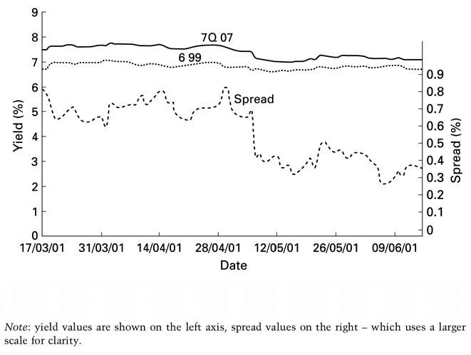
An investor believes that the yield curve will flatten between the 2-year and 10-year sectors of the curve and that the spread between the 6 % 1999 and the 7.25 % 2007 will narrow further from its present value of 0.299%.
To reflect this view the investor buys the 10-year bond and sells short the 2-year bond, in amounts that leave the trade first-order risk-neutral. If we assume the investor buys £1 million nominal of the 7.25% 2007 gilt, this represents an exposure of £1,230.04 loss (profit) if there is a 1-basis-point increase (decrease) in yields. Therefore, the nominal amount of the short position in the 6% 1999 gilt must equate this risk exposure. The BPV per £1 million nominal of the 2-year bond is £166.42, which means that the investor must sell (1230.04/166.42) or £7.3912 million of this bond, given by a simple ratio of the two BPVs. We expect to sell a greater nominal amount of the shorter dated gilt because its risk exposure is lower. This trade generates cash because the short sale proceeds exceed the long buy purchase funds, which are, respectively:
| • | Buy £1m 7.25% 2007: | -£1,102,500; |
| • | Sell £7.39m 6% 1999: | +£7,437,025. |
What are the possible outcomes of this trade? If there is a parallel shift in the yield curve, the trade neither gains or loses. If the yield spread narrows by, say, 15 basis points, the trade will gain either from a drop in yield on the long side or a gain in yield in the short side, or a combination of both. Conversely, a widening of the spread will result in a loss. Any narrowing spread is positive for the trade, while any widening is harmful.
The trade would be put on the same ratio if the amounts were higher, which is scaling the trade. So, for example, if the investor had bought £100 million of the 7.25% 2007, he would need to sell short £739 million of the 2-year bonds. However, the risk exposure is greater by the same amount, so that in this case the trade would generate 100 times the risk. As can be imagined, there is a greater potential reward but at the same time a greater amount of stress in managing the position.
Using BPVs to risk-weight a relative value trade is common but suffers from any traditional duration-based measure because of the assumptions used in the analysis. Note that when using this method the ratio of the nominal amount of the bonds must equate the reciprocal of the bonds’ BPV ratio. So, in this case the BPV ratio is (166.42/1,230.04) or 0.1353, which has a reciprocal of 7.3912. This means that the nominal values of the two bonds must always be in the ratio of 7.39 : 1. This weighting is not static, however; we know that duration measures are a static (snapshot) estimation of dynamic properties such as yield and term to maturity. Therefore, for anything but very short-term trades the relative values may need to be adjusted as the BPVs alter over time, so-called dynamic adjustment of the portfolio.
Another method to weight trades is by duration-weighting, which involves weighting in terms of market values. This compares with the BPV approach which provides a weighting ratio in terms of nominal values. In practice, the duration approach does not produce any more accurate risk weighting.
A key element of any relative value trade is the financing cost of each position. This is where the repo market in each bond becomes important. In the example just described, the financing requirement is: repo out the 7.25% 2007, for which £1.1 million of cash must be borrowed to finance the purchase; the trader pays the repo rate on this stock; and reverse-repo the 6% 1999 bond, which must be borrowed in repo to cover the short sale; the trader earns the repo rate on this stock.
If the repo rate on both stocks is close to the general repo rate in the market, there will be a bid-offer spread to pay but the greater amount of funds lent out against the 6% 1999 bond will result in a net financing gain on the trade whatever happens to the yield spread. If the 7.25% 2007 gilt is special, because the stock is in excessive demand in the market (for whatever reason), the financing gain will be greater still. If the 6% 1999 is special, the trade will suffer a financing loss.
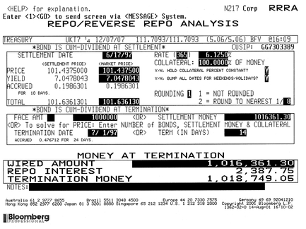
In this case, however, the cash sums involved for each bond make the financing rates academic, as the amount paid in interest in the 7.25% 2007 repo is far outweighed by the interest earned on cash lent out when undertaking reverse repo in the 6% 1999 bond. Therefore, this trade will not be impacted by repo rate bid-offer spreads or specific rates, unless the rate on the borrowed bond is excessively special.52 The repo financing cash flows for the 6% 1999 and 7.25% 2007 are shown in Figures 13.4 and 13.5, respectively, the Bloomberg repo/ reverse repo screen RRRA. They show that at the time of the trade the investor had anticipated a 14-day term for the position before reviewing it and/or unwinding it.
A detailed account of the issues involved in financing a spread trade is contained in Choudhry (2002b).53
Figure 13.4 Bloomberg screen RRRA showing repo cash flows for 6% 1999, 17 June to 1 July 1997.
© Bloomberg Finance L.P. All rights reserved. Used with permission.
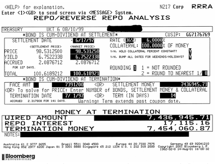
Figure 13.5 Bloomberg screen RRRA showing repo cash flows for 7.25 % 2007, 17 June to 1 July 1997.
© Bloomberg Finance L.P. All rights reserved. Used with permission.
Identifying yield spread trades
Yield spread trades are a type of relative value position that a trader can construct when the objective is to gain from a change in the spread between two points on the yield curve. The decision on which sectors of the curve to target is an important one and is based on a number of factors. An investor may naturally target, say, the 5- and 10-year areas of the yield curve to meet investment objectives and have a view on these maturities. Or a trader may draw conclusions from studying the historical spread between two sectors.
Yield spreads do not move in parallel, however, and there is not a perfect correlation between the changes of short-, medium- and long-term sectors of the curve. The money market yield curve can sometimes act independently of the bond curve. Table 13.1 shows the change in benchmark yields during 1996/1997. There is no set pattern in the change in both yield levels and spreads. It is apparent that one segment of the curve can flatten while another is steepening, or remains unchanged.
Another type of trade is where an investor has a view on one part of the curve relative to two other parts of the curve. This can be reflected in a number of ways, one of which is the butterfly trade, which is considered below.
Table 13.1 Yield levels and yield spreads between November 1996 and November 1997.
Source: ABN Amro Hoare Govett Sterling Bonds Ltd, Hambros Bank Limited; Tullett & Tokyo; author’s notes.

COUPON SPREADS54
Coupon spreads are becoming less common in the gilt market because of the disappearance of high-coupon or other exotic gilts and the concentration on liquid benchmark issues. However, they are genuine spread trades. The US Treasury market presents greater opportunity for coupon spreads due to the larger number of similar-maturity issues. The basic principle behind the trade is a spread of two bonds that have similar maturity or similar duration but different coupons.
Figure 13.6 shows the yields for a set of high-coupon and low(er)-coupon gilts for a specified date in May 1993 and the yields for the same gilts 6 months later. From the yield curves we see that general yield levels decline by approximately 80—130 basis points. The last column in the table shows that, apart from the earliest pair of gilts (which do not have strictly comparable maturity dates), the performance of the lower coupon gilt exceeded that of the higher coupon gilt in every instance. Therefore, buying the spread of the low-coupon versus the high-coupon should, in theory, generate a trading gain in an environment of falling yields. One explanation for this is that the lower coupon bonds are often the benchmark, which means the demand for them is higher. In addition, during a bull market, more bonds are considered to be ‘high’ coupon as overall yield levels decrease.
The exception noted in Figure 13.6 is the outperformance of the 14% Treasury 1996 compared with the lower coupon  1995 stock. This is not necessarily conclusive, because the bonds are 6 months apart in maturity, which is a significant amount for short-dated stock. However, in an environment of low or falling interest rates, shorter dated investors such as banks and insurance companies often prefer to hold very high-coupon bonds because of the high income levels they generate. This may explain the demand for the 14% 1996 stock55 although the evidence at the time was only anecdotal.
Figure 13.6 Yield changes on high- and low-coupon gilts from May 1993 to November 1993.
Source: ABN Amro Hoare Govett Sterling Bonds Ltd; Bloomberg; author’s notes.

BUTTERFLY TRADES56
Butterfly trades are another method by which traders can reflect a view on changing yield levels without resorting to a naked punt on interest rates. They are another form of relative value trade; amongst portfolio managers they are viewed as a means of enhancing returns. In essence, a butterfly trade is a short position in one bond against a long position of two bonds, one of shorter maturity and the other of longer maturity than the short-sold bond. Duration-weighting is used so that the net position is first-order risk-neutral, and nominal values are calculated such that the short sale and long purchase cash flows net to 0, or very closely to 0.
This section reviews some of the aspects of butterfly trades.
Basic concepts
A butterfly trade is par excellence a yield curve trade. If the average return on the combined long position is greater than the return on the short position (which is a cost) during the time the trade is maintained, the strategy will generate a profit. It reflects a view that the short-end of the curve will steepen relative to the ‘middle’ of the curve while the long-end will flatten. For this reason higher convexity stocks are usually preferred for the long positions, even if this entails a loss in yield. However, the trade is not ‘risk-free’, for the same reasons that a conventional two-bond yield spread is not. Although, in theory, a butterfly is risk-neutral with respect to parallel changes in the yield curve, changes in the shape of the curve can result in losses. For this reason the position must be managed dynamically and monitored for changes in risk relative to changes in the shape of the yield curve.
In a butterfly trade the trader is long a short-dated and long-dated bond, and short a bond of a maturity that falls in between these two maturities. A portfolio manager with a constraint on running short positions may consider this trade as a switch out of a long position in the medium-dated bond and into duration-weighted amounts of the short-dated and long-dated bond. However, it is not strictly correct to view the combined long position to be an exact substitute for the short position; due to liquidity (and other reasons) the two positions will behave differently for given changes in the yield curve. In addition, one must be careful to compare like for like, as the yield change in the short position must be analysed against yield changes in two bonds. This raises the issue of portfolio yield.
Putting on the trade
We begin by considering the calculation of the nominal amounts of the long positions, assuming a user-specified starting amount in the short position. In Table 13.2 we show three gilts as at 27 June 1997. The trade we wish to put on is a short position in the 5-year bond, the 7% Treasury 2002, against long positions in the 2-year bond, the 6% Treasury 1999 and the 10-year bond, the  Treasury 2007. Assuming £10 million nominal of the 5-year bond, the nominal values of the long positions can be calculated using duration, modified duration or BPVs (the last two, unsurprisingly, will generate identical results). The more common approach is to use BPVs.
Table 13.2 Bond values for butterfly strategy.
Source: Author’s notes.

In a butterfly trade the net cash flow should be as close to 0 as possible, and the trade must be BPV-neutral. Let us use the following notation:
| P1 | Dirty price of the short position; |
| P2 | Dirty price of the long position in the 2-year bond; |
| P3 | Dirty price of the long position in the 10-year bond; |
| M1 | Nominal value of short-position bond, with M2 and M3 the long-position bonds; |
| BPV1 | Basis point value of the short-position bond. |
Now, if applying BPVs, the amounts required for each stock are given by: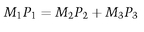 while the risk-neutral calculation is given by:
(13.1)
(13.2)
The value of M1 is not unknown, as we have set it at £10 million. The equations can be re-arranged to solve for the remaining two bonds, which are: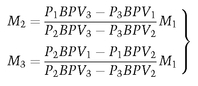
(13.3)
Using the dirty prices and BPVs from Table 13.2, we obtain the following values for the long positions. The position required is short £10 million 7% 2002 and long £5.347 million of the 6% 1999 and £4.576 million of the  2007. With these values the trade results in a zero net cash flow and a first-order, risk-neutral, interest-rate exposure. Identical results would be obtained using the modified duration values, and similar results using the duration measures. If using Macaulay duration the nominal values are calculated using:
 where
where
(13.4)
D = Duration for each respective stock; MV = Market value for each respective stock.
Yield gain
We know that the gross redemption yield for a vanilla bond is that rate r where:
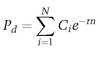
The right-hand side of equation (13.5) is simply the present value of the cash flow payments C to be made by the bond in its remaining lifetime. Equation (13.5) gives the continuously compounded yields to maturity; in practice, users define a yield with compounding interval m, that is:
(13.6)
Treasuries and gilts compound on a semiannual basis.
In principle, we may compute the yield on a portfolio of bonds exactly as for a single bond, using equation (13.5) to give the yield for a set of cash flows which are purchased today at their present value. In practice, the market calculates portfolio yield as a weighted average of the individual yields on each of the bonds in the portfolio. This is described, for example, in Fabozzi (1993), and this description points out the weakness of this method. An alternative approach is to weight individual yields using bonds’ BPVs, which we illustrate here in the context of the earlier butterfly trade. In this trade we have:
• short £10 million 7% 2002;
• long £5.347 million 6% 1999 and £4.576 million  2007.
2007.
Using the semiannual adjusted form of equation (13.5) the true yield of the long position is 7.033%. To calculate the portfolio yield of the long position using market value weighting, we may use: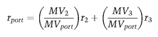 which results in a portfolio yield for the long position of 6.993%. If we weight the yield with BPVs we use:
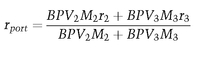
(13.7)
(13.8)
Substituting the values from Table 13.2 we obtain:
We see that using BPVs produces a seemingly more accurate weighted yield, closer to the true yield computed using the expression above. In addition, using this measure a portfolio manager switching into the long butterfly position from a position in the 7% 2002 would pick up a yield gain of 1.2 basis points, compared with the 4 basis points that an analyst would conclude had been lost using the first yield measure.57
The butterfly trade therefore produces a yield gain in addition to the capital gain expected if the yield curve changes in the anticipated way.
Convexity gain
In addition to yield pick-up, the butterfly trade provides, in theory, a convexity gain which will outperform the short position irrespective of which direction interest rates move in, provided we have a parallel shift. This is illustrated in Table 13.3. This shows the changes in value of the 7% 2002 as interest rates rise and fall, together with the change in value of the combined portfolio.
We observe from Table 13.3 that whatever the change in interest rates, up to a point, the portfolio value will be higher than the value of the short position, although the effect is progressively reduced as yields rise. The butterfly will always gain if yields fall and protects against downside risk if yields rise to a certain extent. This is the effect of convexity; when interest rates rise the portfolio value declines by less than the short position value, and when rates fall the portfolio value increases by more. Essentially, the combined long position exhibits greater convexity than the short position. The effect is greater if yields fall, while there is an element of downside protection as yields rise, up to the +150-basis-point parallel shift.
Table 13.3 Changes in bond values with changes in yield levels.

Portfolio managers may seek greater convexity whether or not there is a yield pick-up available from a switch. However, the convexity effect is only material for large changes in yield, and so if there was not a corresponding yield gain from the switch, the trade may not perform positively. As we noted, this depends partly on the funding position for each stock. The price/yield profile for each stock is shown in Figure 13.7.
Essentially, by putting on a butterfly as opposed to a two-bond spread or a straight directional play, the trader limits the downside risk if interest rates fall, while preserving the upside gain if yields fall.
To conclude the discussion of butterfly trade strategy, we describe the analysis using the BBA screen on Bloomberg. The trade is illustrated in Figure 13.8.
Using this approach, the nominal values of the two long positions are calculated using BPV ratios only. This is shown under the column ‘Risk Weight’, and we note that the difference is 0. However, the nominal value required for the 2-year bond is much greater at £10.76 million, and for the 10-year bond much lower at £2.8 million. This results in a cash outflow of £3.632 million. The profit profile is, in theory, much improved; at the bottom of the screen we observe the results of a 100-basis-point parallel shift in either direction, which is a profit. Positive results were also seen for 200- and 300-basis-point parallel shifts in either direction. This screen incorporates the effect of a (uniform) funding rate, input on this occasion as 6.00%.58 Note that the screen allows the user to see the results of a pivotal shift; however, in this example a 0-basis-point pivotal shift is selected.
Figure 13.7 Illustration of convexity for each stock in butterfly trade, 27 June 1997.
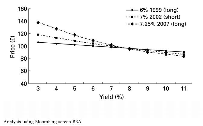
Figure 13.8 Butterfly trade analysis on 27 June 1997, on screen BBA.
© 1997 Bloomberg Finance L.P. All rights reserved. Used with permission.

Figure 13.9 Butterfly trade spread history.
© Bloomberg Finance L.P. All rights reserved. Used with permission.

This trade therefore created a profit whatever direction interest rates moved in, assuming a parallel shift.
The spread history for the position up to the day before the trade is shown in Figure 13.9, a reproduction of the graph on Bloomberg screen BBA.
BLOOMBERG SCREENS
We illustrate two Bloomberg screens that can be used for both government and corporate bonds analysis here. The first is BQ which is a combination of a number of analytics and metrics.
To call up the screen we type the specific followed by <BQ>. So in this case for the 5% 2012 gilt we type:
UKT 5 12 <GOVT> <BQ> GO
Figure 13.10 is a page of the screen BQ and shows the bond price, plus a number of yield spreads. The G-spread is the yield below the government benchmark, which as we expect, given that this is a government bond, is very small. The I-spread is the spread to the interest-rate swap curve, in this case negative because it is a risk-free government bond. The three other spreads are:
• ASW - the asset swap spread, which is the spread payable above (or below) Libor if constructing an asset swap for this bond using an interest-rate swap to convert its coupon from fixed rate to floating rate.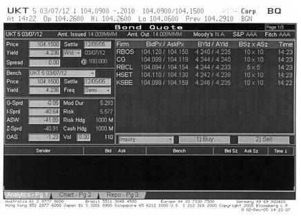
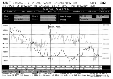
Figure 13.10 Bloomberg screen BQ, page 1, for UK gilt 5% 2012, as at 2 December 2005.
© 2005 Bloomberg Finance L.P. All rights reserved. Used with permission.
Figure 13.11 Bloomberg screen BQ, page 2, for UK gilt 5 % 2012, as at 2 December 2005.
© 2005 Bloomberg Finance L.P. All rights reserved. Used with permission.
• Z-spread - the spread to the swap curve but using appropriate zero-coupon rates to discount each bond’s cash flow rather than the uniform swap rate for the bond’s maturity.
• OAS - the option-adjusted spread, the spread required to equate the bond’s cash flows to its current price after adjusting for the effect of any embedded options (e.g., early redemption as with a callable bond); this is minimal with a bullet maturity gilt.
The right-hand side of page 1 of screen BQ shows some contributing prices from five banks or brokers.
For a full explanation of the use of these spread measures in corporate bond relative value analysis see Choudhry (2005).
Page 2 of the same screen at Figure 13.11 shows historical yield spreads, in this case the yield to maturity against the asset swap spread. The time period shown is user-selected.
Page 3 of the screen is a funding calculator, shown at Figure 13.12. We see here that for this holding of the bond the term is overnight and the nominal amount is £1 million.
Figure 13.12 Bloomberg screen BQ, page 3, for UK gilt 5 % 2012, as at 2 December 2005.
© 2005 Bloomberg Finance L.P. All rights reserved. Used with permission.

Page 4 of the screen is a credit ratings related page. Such a page is not shown for a gilt because it is seen as risk-free, so we illustrate it using the Ford 2.25% 2007 bond we introduced in Chapter 1. This is shown at Figure 13.13. We see the Moody’s and S&P’s ratings as well as ratings analyst fundamental data on the bond.
The screen YCRV shows a number of yield curve screens. For example, the user can select up to four different curves for historical comparison. We show this at Figure 13.14, which is screen YCRV selected with the US Treasury, USD Libor, US Term Fed Funds and the UK government benchmark shown. This is as at 2 December 2005. The large-size graph is shown at Figure 13.15.
BOND SPREADS AND RELATIVE VALUE
Return from a holding of fixed income securities may be measured in more than one way. The simplest way is to consider a spread over the government yield curve, interpolating yields where necessary. However, the most common approach is to consider the asset swap spread. More sophisticated investors also consider the basis spread between the cash bond and the same-name credit default swap price, which is known as the basis.59 Using the CDS basis for relative value analysis is considered in Choudhry (2010b). In this section we consider the interpolated spread and the asset swap spread.
Figure 13.13 Bloomberg screen BQ, page 4, for the Ford 2.25 % 2007 MTN, as at 2 December 2005.
© 2005 Bloomberg Finance L.P. All rights reserved. Used with permission.
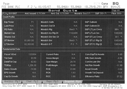
Figure 13.14 Bloomberg screen YCRV showing four US and UK curves, as at 2 December 2005.
© 2005 Bloomberg Finance L.P. All rights reserved. Used with permission.

Figure 13.15 Bloomberg screen YCRV with enlarged graph display, as at 2 December 2005.
© 2005 Bloomberg Finance L.P. All rights reserved. Used with permission.

Bond spreads
Investors measure the perceived market value, or relative value, of a corporate bond by measuring its yield spread relative to a designated benchmark. This is the spread over the benchmark that gives the yield of the corporate bond. A key measure of relative value of a corporate bond is its swap spread. This is the basis point spread over the interest-rate swap curve, and is a measure of the credit risk of the bond. In its simplest form, the swap spread can be measured as the difference between the yield to maturity of the bond and the interest rate given by a straight line interpolation of the swap curve. In practice traders use the asset swap spread as the main measure of relative value. The government bond spread is also used.
The spread that is selected is an indication of the relative value of the bond and a measure of its credit risk. The greater the perceived risk, the greater the spread should be. This is best illustrated by the credit structure of interest rates, which will (generally) show AAA-rated and AA-rated bonds trading at the lowest spreads and BBB-rated, BB-RATED and lower rated bonds trading at the highest spreads. Bond spreads are the most commonly used indication of the risk-return profile of a bond.
In this section we consider the Treasury spread, the asset swap spread and a variant of the asset swap spread known as the Z-spread.
Swap spread and Treasury spread
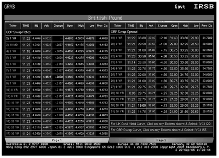
A bond’s swap spread is a measure of the credit risk of that bond, relative to the interest-rate swaps market. Because the swaps market is traded by banks, this risk is effectively the interbank market, so the credit risk of the bond over and above bank risk is given by its spread over swaps. This is a simple calculation to make, and is simply the yield of the bond minus the swap rate for the appropriate maturity swap. Figure 13.16 shows Bloomberg page IRSB for pounds sterling as at 10 August 2005. This shows the GBP swap curve on the left-hand side. The right-hand side of the screen shows the swap rates’ spread over UK gilts. It is the spread over these swap rates that would provide the simplest relative value measure for corporate bonds denominated in GBP. If the bond has an odd maturity, say 5.5 years, we would interpolate between the 5-year and 6-year swap rates.
The spread over swaps is sometimes called the I-spread. It has a simple relationship to swaps and Treasury yields, shown here in the equation for corporate bond yield, where
where
(13.9)
Y = The yield on the corporate bond; I = The I-spread or spread over swap;
S = The swap spread;
T = The yield on the Treasury security (or an inter-
polated yield).
S = The swap spread;
T = The yield on the Treasury security (or an inter-
polated yield).
Figure 13.16 Bloomberg page IRSB for pounds sterling, showing GBP swap rates and swap spread over UK gilts.
© Bloomberg Finance L.P. All rights reserved. Used with permission.
In other words, the swap rate itself is given by T + S.
The I-spread is sometimes used to compare a cash bond with its equivalent CDS price, but for straightforward relative value analysis it is usually dropped in favour of the asset swap spread, which we look at later in this section.
Of course the basic relative value measure is the Treasury spread or government bond spread. This is simply the spread of the bond yield over the yield of the appropriate government bond. Again, an interpolated yield may need to be used to obtain the right Treasury rate to use. The bond spread is given by:
BS = Y - T.
Using an interpolated yield is not strictly accurate because yield curves are smooth in shape, and so straight line interpolation will produce slight errors. The method is still commonly used though.
Asset swap spread
An asset swap is a package that combines an interest-rate swap with a cash bond, the effect of the combined package being to transform the interest-rate basis of the bond. Typically, a fixed rate bond will be combined with an interest-rate swap in which the bondholder pays fixed coupon and receives floating coupon. The floating coupon will be a spread over Libor (see Choudhry et al., 2001). This spread is the asset swap spread and is a function of the credit risk of the bond over and above interbank credit risk.60 Asset swaps may be transacted at par or at the bond’s market price, usually par. This means that the asset swap value is made up of the difference between the bond’s market price and par, as well as the difference between the bond coupon and the swap fixed rate.
The zero-coupon curve is used in the asset swap valuation. This curve is derived from the swap curve, so it is the implied zero-coupon curve. The asset swap spread is the spread that equates the difference between the present value of the bond’s cash flows, calculated using the swap zero rates, and the market price of the bond. This spread is a function of the bond’s market price and yield, its cash flows and the implied zero-coupon interest rates.61
Consider a bond whose price was observed on Bloomberg on 10 August 2005, GKN Holdings 7% 2012, with an asset swap spread of 121.5 basis points. This is the spread over Libor that will be received if the bond is purchased in an asset swap package. In essence the asset swap spread measures a difference between the market price of the bond and the value of the bond when cash flows have been valued using zero-coupon rates. The asset swap spread can therefore be regarded as the coupon of an annuity in the swap market that equals this difference.
Z-spread
The conventional approach for analysing an asset swap uses the bond’s yield to maturity (YTM) in calculating the spread. The assumptions implicit in the YTM calculation, noted in chapter 6 of Choudhry (2001), make this spread problematic for relative analysis, so market practitioners use what is termed the Z-spread instead. The Z-spread uses the zero-coupon yield curve to calculate spread, so is a more realistic, and effective, spread to use. The zero-coupon curve used in the calculation is derived from the interest-rate swap curve.
Put simply, the Z-spread is the basis point spread that would need to be added to the implied spot yield curve such that the discounted cash flows of a bond are equal to its present value (its current market price). Each bond cash flow is discounted by the relevant spot rate for its maturity term. How does this differ from the conventional asset swap spread? Essentially, in its use of zero-coupon rates when assigning a value to a bond. Each cash flow is discounted using its own particular zero-coupon rate. The price of a bond at any time can be taken to be the market’s value of the bond’s cash flows. Using the Z-spread we can quantify what the swap market thinks of this value (i.e., by how much the conventional spread differs from the Z-spread). Both spreads can be viewed as the coupon of a swap market annuity of equivalent credit risk of the bond being valued.
In practice, the Z-spread, especially for shorter dated bonds and for better credit quality bonds, does not differ greatly from the conventional asset swap spread. The Z-spread is usually the higher spread of the two, following the logic of spot rates, but not always. If it differs greatly, then the bond can be considered to be mispriced.
The Z-spread is closely related to the bond price, as shown by: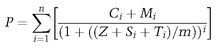 where
where
(13.10)
n = The number of interest periods until maturity; P = The bond price;
C = The coupon;
C = The coupon;
M = The redemption payment (so bond cash flow is all C plus M);
Z = The Z-spread;
m = The frequency of coupon payments.
m = The frequency of coupon payments.
In effect this is the standard bond price equation with the discount rate adjusted by whatever the Z-spread is; it is an iterative calculation. The appropriate maturity swap rate is used, which is the essential difference between the I-spread and the Z-spread. This is deemed to be more accurate, because the entire swap curve is taken into account rather than just one point on it. In practice though, as we have seen in the example above, there is often little difference between the two spreads.
To reiterate then, using the correct Z-spread, the sum of the bond’s discounted cash flows will be equal to the current price of the bond.
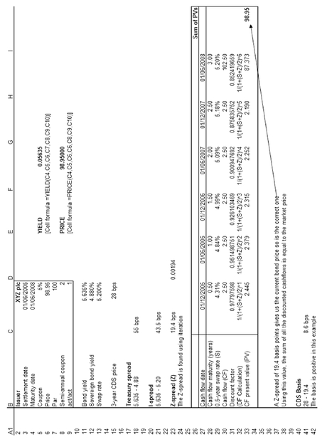
We illustrate the Z-spread calculation at Figure 13.17. This is done using a hypothetical bond, the XYZ plc 5% of June 2008, a 3-year bond at the time of the calculation. Market rates for swaps, Treasuries and CDSs are also shown. We require the spread over the swaps curve that equates the present values of the cash flows to the current market price. The cash flows are discounted using the appropriate swap rate for each cash flow maturity. With a bond yield of 5.635%, we see that the I-spread is 43.5 basis points, while the Z-spread is 19.4 basis points. In practice the difference between these two spreads is rarely this large.
For the reader’s benefit we also show the Excel formula at Figure 13.17. This shows how the Z-spread is calculated; for ease of illustration we have assumed that the calculation takes place for value on a coupon date, so that we have precisely an even period to maturity.
Summary of a fund manager’s approach to value creation
The management of a portfolio of bonds may be undertaken either passively or actively. Passive fund management does not involve any actual analysis or portfolio selection, because the manager merely constructs the bond portfolio to mirror the benchmark or index whose performance he wishes to replicate, as such passive fund management is more of an administrative function than an analytical or strategic one.
Active fund management involves just that: the manager makes the decision on which bonds to buy and the time at which to buy (and subsequently sell) them. The performance of an actively managed fixed income portfolio is still measured against the relevant benchmark or index, because this serves to illustrate how well the manager is doing. If the portfolio does not outperform the index, then the manager has not added value.
Figure 13.17 Calculating the Z-spread, hypothetical 5% 2008 bond issued by XYZ plc
What approach is adopted by the active fund manager? Portfolio managers employ four basic strategies to add value over and above the benchmark. We summarise these here:
• Extend duration before a market rally, shorten duration before a market correction: this is the most basic approach, and in its crudest form amounts to ‘punting’ the market. The fund manager basically decides when he expects the market to rally and buys longer dated bonds ahead of the anticipated move upwards, which benefit from such a move more than shorter dated bonds. Unfortunately, very few fund managers consistently get such a call right and this approach is not often adopted, at least not explicitly anyway.
• Yield curve trades: in this approach the fund manager puts on steepening trades before the yield curve steepens and flattening trades before the curve flattens. A common approach is to put on barbell and bullet trades; generally the former are adopted for curve-flattening trades, while a steepening yield curve tends to favour bullet trades. This strategy has a bit more intellectual cachet than the straight directional ‘punt’ trade, and generally fund managers are given more latitude to put on relative value-style curve-shaping trades compared with directional trades. However, ultimately this approach also calls for the manager to call the directional move in the market right.
• Convexity and volatility trades: this strategy also has a directional element to it, and involves employing convexity and volatility trades to outperform benchmarks. When there is a mismatch between a manager’s view on volatility and the implied volatility of bonds with embedded options, buying or selling convexity before realised volatility increases or decreases can enhance return. An alternative approach is, rather than realised volatility differing from implied volatility, the market as a whole may change its opinion about future volatility and thereby produce a change in implied volatility, which may enhance returns. Convexity and volatility trades can also be effected using barbell and bullet positions, or via derivatives.
• Security selection: portfolio managers can attempt to outperform benchmarks through security selection. This entails being overweight in ‘cheap’ bonds and underweight in ‘rich’ bonds, which will produce higher total return relative to the benchmark. Security selection requires effective relative value analysis to determine which bonds are cheap compared with their peer group and with the risk-free benchmark. Such analysis makes use of measures such as the asset swap spread. A basic analysis would use this metric and compare it across an (otherwise equivalent) set of bonds. The approach is as follows: after selecting portfolio average duration and the level of credit risk that is acceptable, purchase the bonds that have the highest asset swap spread. The resulting portfolio then represents the best relative value for a given duration target and credit risk exposure. In practice, the asset swap spread is nowadays also compared with the same-name credit default swap premium. The difference between the two measures (the CDS basis) gives another measure of the relative value of the bond, by implying the level of mispricing in either or both of the cash and synthetic markets.
Active fund management, whichever method or combination of methods is adopted, ultimately still requires the manager to have an idea of market direction. If the fund manager gets this right, this makes it more likely that the portfolio will outperform the benchmark.
BIBLIOGRAPHY
Choudhry, M. (2001). The Bond and Money Markets: Strategy, Trading, Analysis. Butterworth-Heinemann, Oxford, UK, ch. 6.
Choudhry, M. (2002). Professional Perspectives on Fixed Income Portfolio Management (Vol. 3, edited by Frank J. Fabozzi). John Wiley & Sons, New York, USA.
Choudhry, M. (2005). Corporate Bond Markets: Instruments and Applications. John Wiley & Sons, Singapore, ch. 15.
Choudhry, M. (2010a). The Repo Handbook (2nd edn). Butterworth-Heinemann, Oxford, UK.
Choudhry, M. (2010b). Structured Credit Products (2nd edn). John Wiley & Sons, Singapore.
Fabozzi, F. (1996). Bond Portfolio Management. FJF Associates, chs 10-14.
..................Content has been hidden....................
You can't read the all page of ebook, please click here login for view all page.