
Chapter 101
LIQUIDITY RISK MANAGEMENT II: BASEL III LIQUIDITY, LIABILITIES STRATEGY, STRESS TESTING, COLLATERAL MANAGEMENT AND THE HQLA
In this chapter we consider an important part of the liquidity risk management process, that of quantifying and reporting liquidity risk exposure as required by the universal “Basel III” rules on bank supervision. We also consider all related ingredients of a best‐practice liquidity risk management framework. This makes Chapter 10 rather a long one, but worth working through as it is possibly the most important in the book!
BASEL III LIQUIDITY METRICS
Strong capital requirements are a necessary condition for banking sector stability but by themselves are not sufficient. A strong liquidity base reinforced through robust supervisory standards is of equal importance. Prior to 2010, there were no internationally harmonised standards in this area. To complement the other elements of its liquidity framework (Principles for Sound Liquidity Risk Management and Supervision and Additional Monitoring Metrics), the Basel Committee developed two minimum liquidity standards:
- The Liquidity Coverage Ratio (LCR): to promote short‐term funding resilience;
- The Net Stable Funding Ratio (NSFR): to provide a sustainable maturity structure of assets and liabilities.
In Europe, a minimum LCR was introduced in October 2015. Implementation of the NSFR, however, is not due until 2018, to give global regulators sufficient time to conduct parallel run exercises to enable proper calibration of the ratio.
Liquidity coverage ratio
The LCR focuses on the short term and is designed to ensure that a financial institution has sufficient unencumbered high‐quality liquid resources to survive a severe liquidity stress scenario lasting for 1 month. The ratio is calculated as:
Stock of high‐quality liquid assets/Total net cash outflows over the next 30 days (in a stress situation) ≥ 100%
The highest quality liquid assets (for example, cash or government bonds) are included in the calculation at their market value. Assets of a slightly lower quality, such as covered bonds and securitisation paper, may also be counted if their ratings are above minimum thresholds, but will be subject to a haircut.
Run‐off factors are applied to liabilities and off‐balance‐sheet commitments based on their likelihood of withdrawal/drawdown in a stress. Figure 10.1 provides a simplified overview of the initial assumptions published by the Basel Committee in 2010.

Figure 10.1 Simplified overview of the LCR calculation
© Chris Westcott 2017. Used with permission.
Liquidity stress scenario
The assumptions are provided by the regulatory authorities based upon a combined market and idiosyncratic stress, which incorporates many of the shocks experienced during the financial crisis. They should be viewed as a minimum supervisory requirement for banks. Banks are expected to conduct their own stress tests to assess the level of liquidity they should hold beyond this minimum, and construct their own scenarios that could cause difficulties for their specific business activities. The results of these additional stress tests should be shared with supervisors (Individual Liquidity Adequacy Process and Liquidity Supervisory Review and Evaluation Process are covered in Section 19 of the handbook).
Liquid assets
Liquid assets eligible for inclusion in the calculation were initially split into two categories (Level 1 and Level 2), but this was subsequently increased to three (Level 1, Level 2A, and Level 2B) to capture a broader range of securities:
- Level 1: up to 100% of the total, comprising cash, deposits at the central bank government/government guaranteed bonds, and covered bonds rated ECAI 1 (External Credit Assessment Institutions – EU rating system) that meet certain conditions (subject to a 7% haircut and a 70% cap in the liquidity buffer);
- Level 2A: up to 40% of the total with a minimum haircut of 15%, comprising government bonds with 20% risk weight, EU covered bonds rated ECAI 2, and non‐EU covered/corporate bonds rated ECAI 2;
- Level 2B: up to 15% of the total with a haircut of 25–50%, comprising RMBS, auto, SME, and consumer loan securitisations, corporate bonds rated ECAI 3, shares that are part of a major stock index, and other high‐quality covered bonds.
Cash outflow/inflow assumptions
The rules for the EU, which were finalised in January 2015, contained a number of amendments to the assumptions on cash outflows/inflows:
- From 2019, a new lower outflow rate of 3% for retail deposits (subject to Member State and Commission approval);
- Two new risk buckets for other less stable retail deposits (10–15% and 15–20%);
- Lower outflow assumptions for maturing deposits from non‐financial customers, sovereigns, central banks, and PSEs (20–40%);
- More granularity for outflow assumptions on maturing secured funding transactions;
- Higher outflow assumptions (30–40%) for undrawn committed liquidity facilities to non‐financial corporates provided to replace funding that cannot be obtained in the financial markets;
- More favourable outflow assumptions on deposits from credit unions and undrawn credit or liquidity facilities for members of a group or institutional protection scheme.
The overall effect of the assumption changes has been a net relaxation of the rules, making it easier for banks to comply. As at 31 December 2012, Group 1 Banks (those with Tier 1 capital >€3 bn and internationally active) had an average LCR of 95% based on the 2010 BCBS rules and 119% based on the January 2013 version. As at the same date, Group 2 Banks had an average LCR of 99% based on the 2010 BCBS rules and 126% based on the January 2013 version.
LCR implementation in the US and Switzerland
The US has introduced an LCR that is consistent with that applying in Europe, although it differs in a number of respects. There is an additional feature called a “maturity mismatch add‐on” – it requires institutions to identify the largest single‐day maturity mismatch within the 30‐day period by calculating the daily difference in cumulative outflows and inflows that have set maturity dates. The maturity mismatch add‐on is the difference between the peak day amount and the net cumulative outflow amount on the last day of the 30‐day period. This is illustrated in Figure 10.2 – although the institution in question has a 100% LCR, there is an additional liquid asset holding requirement of US$230m due to the maturity mismatch add‐on.

Figure 10.2 The US maturity mismatch add‐on
The LCR rule only applies to the largest, internationally active US banks. The final rule has been effective since 1 January 2015 (min. 80% compliance), though there is a transitional phase with full application from 1 January 2017 (earlier than under the Basel Committee framework). The LCR rule will be complemented by the NSFR in 2019.
Due to the low level of public debt in Switzerland, “Alternative Liquidity Approaches” are available to enable compliance with minimum ratio requirements. Outflows in Swiss francs can be covered up to a defined portion in foreign currency assets. Also, a higher proportion of Category 2 assets may be permitted and short‐term repo transactions against high‐quality assets with a maturity of less than 30 days may be treated as non‐existent.
The Net Stable Funding Ratio
In contrast to the LCR, the NSFR is a measure of structural liquidity and focuses on the longer‐term horizon by placing a formal limit on the amount of maturity transformation that banks are able to undertake. The required ratio is calculated as:
Available amount of stable funding/Required amount of stable funding ≥100%
All assets (required amount of stable funding) and liabilities (available amount of stable funding) are weighted according to their likelihood of still being on the balance sheet 12 months into the future.
Figure 10.3 gives a simplified overview of the assumptions used in the NSFR calculation based upon the Basel III document. Since the initial calibration, the Basel Committee proposed a number of amendments to the Available Stable Funding (ASF) and Required Stable Funding (RSF) factors in January and October 2014. Some of the main changes were:

Figure 10.3 Simplified overview of the NSFR calculation
© Chris Westcott 2017. Used with permission.
- The ASF factor on operational deposits was increased from 0% to 50%;
- The ASF factor on stable retail and SME deposits was increased from 90% to 95%;
- The RSF factor was increased from 0% to 50% on both non‐renewable loans to non‐bank financial institutions with a maturity of less than 1 year and inter‐bank lending for a period of 6 months to 1 year;
- Net derivative liabilities are included in the 0% ASF category and 20% of derivative liabilities captured in the 100% RSF category (as well as net derivative assets);
- Two new RSF categories have been introduced at 10% and 15% for unencumbered loans to financial institutions (previously 0%).
The implications of the Basel liquidity metrics for banks' funding and lending strategies
The new rules combined with banks' own desire to reduce liquidity risk have resulted in material changes in balance sheet structures. The adjustment process began in 2008, so is now well advanced. Initially, LCR/NSFR presented a compliance issue, but satisfying the ratios on an ongoing basis is increasingly becoming an efficiency issue.
Some of the main impacts have included:
- Customer loan/deposit ratios moving more into balance;
- A reduction in inter‐bank loan/deposit market and repo activity (except in government securities);
- A focus on retail/SME deposits, including the introduction/relaunch of deposit products, such as 35‐day notice accounts;
- Simplification of balance sheet structures to reduce trapped liquidity in branches and/or subsidiaries;
- Higher liquid asset holdings and disposal of traded securities that do not count towards the LCR;
- Tighter control of undrawn commitments, particularly liquidity facilities, where the treatment is asymmetric;
- Increased consideration of the currency denomination of activities;
- The generation of liquidity from long‐term assets.
For efficient balance sheet optimisation, a bank should consider how the above impacts its business model and specific business lines, and seek to concentrate on those areas that provide efficiency in both return and regulatory compliance.
OPTIMUM LIABILITIES STRATEGY AND MANAGING THE HIGH‐QUALITY LIQUID ASSETS (HQLA) PORTFOLIO
In this section we examine the interdependency between the liability strategy and the link that it has to the HQLA, known in pre‐Basel III days as the liquidity book or liquid asset buffer (LAB), requirement.
Liabilities strategy
As part of an integrated liquidity risk management framework, a bank should articulate an optimum liabilities strategy. This sits at the heart of the balance sheet planning process. The liabilities strategy of an organisation needs to take into consideration the diversification of the liability base to ensure that it is not concentrated in any particular aspect such as tenor, client, industry sector, or product type.
Under the strategic asset‐liability management (ALM) umbrella, there are a few core components that are directly relevant to the liabilities strategy:
- A single, integrated balance sheet approach that ties in asset origination with liabilities raising;
- Thus, asset type must be relevant and appropriate to funding type and source…;
- …and the funding type and source must be appropriate to the asset type.
In order to apply these three key principles, it is important to undertake a comprehensive review of the bank's balance sheet liabilities as a first step towards determining both the optimum liability profile and then the overall liabilities strategy.
This exercise is more involved in the larger and more complex businesses, but critical nonetheless.
The strategy setting is not a static or one‐off process. The objective is to arrive at a balance sheet liability mix and structure by design, and one which is optimum from a strategic ALM perspective, rather than one that is a result simply of history and business line BAU activity – in other words, a passive inherited liability shape.
The changing liabilities structure of banks
Let's examine how bank balance sheets have evolved over time in order to better understand the context of a liabilities strategy. Figure 10.4 shows the changes in breakdown of funding types that took place with UK banks between 2007 and 2012.
| UK banks' average | |||
| 2007 | 2012 | ||
| Deposits by banks | 6.00% | 3.80% | |
| Customer accounts | 31% | 31% | |
| Debt securities | 12.30% | 10.60% | |
| NIBLs | 24.30% | 27.50% | |
| Equity | 4.40% | 5.00% | |
| Other | 21.90% | 22.10% | |
| Total liabilities and equity | 100% | 100% | |
| (Source: SEC 20‐F filings) | |||
Figure 10.4 Funding breakdown of UK banks' average, 2007 and 2012
The liability structure of many EU and MENA banks have changed since 2007–2008 and have focused on moving away from wholesale funds, both short term (supply) and long term (demand), and move towards more non‐interest bearing liabilities (NIBLs) and equity. This has largely been driven by the introduction of the ILAS regime and subsequent LCR stress testing regulatory metrics. Both of these stress tests penalise the use of wholesale funding and hence banks have diversified and focused on retail and NIBLs balances. For one high street UK bank, NIBLs rose from 28% of liabilities and equity in 2007 to 41% in 2012.
The liability structure: what is the optimum mix?
In compiling the optimum liability mix targets, there are some important considerations that need to be applied in the planning process. These revolve around:
- Regulation;
- Liquidity value (to what extent is a type of customer deposit or type beneficial towards the final LCR or NSFR metric?);
- Funding diversification/concentration;
- Impact to net interest income (NII) and net interest margin (NIM);
- NII sensitivity;
- How to build the customer franchise;
- Set up costs of new products.
Figure 10.5 highlights the detailed considerations that need to be applied during the planning process.
| Factor | Consideration |
| Regulation | Deposit Guarantee Scheme? Is a regulated sales force required to distribute the product? |
| Liquidity | What is the liquidity value of the deposit? |
| Concentration | Does the deposit type improve the diversity of the funding base? |
| NII/NIM | Contribution to NII per funds transfer pricing (FTP) system, not gross cost? |
| NII sensitivity | Does the deposit act as a natural hedge for assets? Some banks do not use derivatives to manage NII sensitivity |
| Customer franchise | Does the product reinforce the franchise value of the organisation? E.g., Santander 123 account |
| Other costs | Explicit costs associated with the product? |
Figure 10.5 Considerations during the liabilities strategy setting stage
Banks fund their balance sheets using a variety of liability types. The liquidity value of each type is different. Ideally, a funding type has high liquidity value as well as high NII value, customer franchise value, etc. This is essentially the “strategic ALM” optimisation problem, attempting to structure the balance sheet mix, in this case with respect to liabilities, that best serves the competing requirements of the regulator, the customer stakeholder, and the shareholder.
In practice, there is usually a trade‐off among these factors as some liabilities have greater term liquidity value for a bank than others. At one end of the scale are retail current accounts; at the other end are short‐term unsecured wholesale liabilities, sourced in the inter‐bank market, which have much more volatile characteristics in stressed market conditions and therefore are less valuable for liquidity management purposes.
Figure 10.6 illustrates the hierarchy of value of different types of liabilities. From a liquidity value perspective, a bank should seek to maximise funding from customer relationship balances and minimise its reliance on wholesale inter‐bank funding.

Figure 10.6 Liquidity value of liabilities
Source: Choudhry (2012)
The mix of these should be arrived at through design as much as possible and a bank's FTP process may be used to help drive liabilities raising of the “right” type and through incentivising businesses by rewarding them with a higher commission or sales credit for the higher value liquidity type.
Peer group analysis
In the UK, the Bank of England (BoE) publishes monthly data showing effective interest‐rate paid on (sterling) deposit balances of UK household and UK non‐FI corporate sectors, split by deposit type. It is a measure of back‐book deposit costs (in the UK), not front book (i.e. marginal cost of new funds).
Through this peer review, one can compare the current bank levels to peer levels to establish whether your bank is paying above the sector‐wide average and to establish a better understanding of what your bank is paying for its deposits and assess if this can be improved.
From Figure 10.7, we observe that for UK banks, 2‐year fixed‐rate bonds have reduced by ∼200bp since 2010, from an average of 3.25% to 1.46%. For instant access liability products, this has reduced by ∼90bp from 1.44% to 0.54%.
| Bank of England Statistics | ||||||
| 2‐year fixed‐rate bonds (%) | Instant access including bonus (%) | Instant access excluding bonus (%) | ISA including bonus (%) | ISA excluding bonus (%) | 1‐year fixed‐rate ISA (%) | |
| 2010 | 3.25 | |||||
| 2011 | 3.27 | 1.44 | 0.51 | 2.48 | 1.25 | 2.56 |
| 2012 | 3.02 | 1.45 | 0.48 | 2.46 | 1.35 | 2.54 |
| 2013 | 1.99 | 0.86 | 0.50 | 1.46 | 0.71 | 1.77 |
| 2014 | 1.60 | 0.67 | 0.46 | 1.17 | 0.86 | 1.49 |
| 2015 | 1.46 | 0.54 | 0.39 | 1.00 | 0.82 | 1.41 |
Figure 10.7 BoE comparative rates statistics example
In addition to data published by central banks, a bank should survey the market itself to determine the current pricing associated with certain liability products. In Figure 10.8 we present the results of such a comparison. We note that “XYZ bank” is exactly where it most probably wishes to be, in the middle of the range among its peers and not an outlier for rates at either end. The highest deposit rate payers are sometimes perceived by customers to be struggling to raise deposits, and such a customer perception would not be welcome for a bank.
| Deposit terms | ABC Bank | XYZ Bank | County Bank | Friendly Bank | Life Bank | Trust Bank |
| Instant access | 0.10 | 1.50 | 0.50 | 0.95 | 0.90 | |
| 30‐day notice | 1.25 | 0.60 | 1.00 | 1.35 | 1.10 | 1.00 |
| 90‐day notice | 1.55 | 2.00 | 1.75 | 0.95 | 1.35 | |
| 95‐day notice | 1.95 | 2.00 | 1.35 | |||
| 3‐month | 1.55 | 2.00 | ||||
| 6‐month | 2.00 | 1.75 | 2.25 | 2.25 | 1.75 | |
| 12‐month | 2.20 | 2.15 | 2.50 | 2.65 | 2.00 | |
| 2‐year | 2.35 | 2.50 | ||||
| 3‐year | 2.60 | |||||
| 5‐year | 2.65 |
Figure 10.8 Deposit rates peer comparison
An analysis of front‐book deposit prices vs competitors would provide additional colour to the liabilities review. This information should also be presented regularly to either the Products Pricing Committee or Deposits Pricing Committee (subcommittee of asset–liability committee (ALCO)). As noted above, the general rule of thumb is not to be an outlier at either end.
Product volume sensitivity to interest‐rate movements
Some liability products are sensitive to movements in interest rates and are referred to as NII‐sensitive products. A high volume sensitivity may not be a good thing as this could lead to certain challenges, notably cannibalisation from other product types and “hot money”.
Cannibalisation from other deposit products offered by the bank can lead to a dramatically different impact on NII than originally anticipated, especially if large volumes of deposits switch to the new/repriced product from high margin accounts. Placing restrictions on who can apply for certain products can attract the attention of the regulators.
“Hot money” from interest‐rate seekers (stand‐alone customers): if a new/repriced account attracts deposits from customers who are only interested in the rate being paid, then you may finish up with expensive funding that has no liquidity value. For this reason, many banks have withdrawn from offering offshore instant access Internet‐based accounts.
The same can also be said of products that have been offered at below par rate. Deposit products often have tiered rates and/or customer relationship managers are given the discretion to pay a higher rate to protect/attract business. Average product margins can mask underlying trends. Figure 10.9 is an example of this type of review in more detail.

Figure 10.9 Deposit product analysis
As part of the liability strategy, a bank should conduct a granular review to understand which deposits are being written at negative margins and consider the options to reduce the size of this segment of business as it is value destroying.
Output of the liability review
The result of the liabilities mix review should be a medium‐term (for example, 3‐ to 5‐year) strategy that specifies a precise target for:
- The liabilities mix: how much do we wish of each funding type, and why;
- What the drivers are;
- What, if any, funding types are of less value and should be reduced or withdrawn from;
- Plan for implementation.
This liabilities strategy review would be presented for ALCO approval and subsequent implementation. This plan could include a series of initiatives that would be tracked at ALCO on a regular basis to ensure that the balance sheet is tracking in the right direction and is being measured by some key performance indicators.
Initiatives could include any or all of those listed in Figure 10.10.
| Initiative | |
| Customer optimisation | Target specific sectors, e.g. universities, charities. Package an offering to growing customer segments |
| Rationalise geographies | |
| Volume caps on retail customer business (e.g. £1m) | |
| Remove from sale any products offering lifetime guarantees | |
| Margin improvement | Increase range of managed rate products by reducing those that price according to a fixed formula (e.g. base rate + ..%) |
| Other initiatives | Stand‐alone customers: target reduction in “rate chaser” customers acquired during periods of aggressive balance sheet growth |
| Lengthen notice period on notice accounts, from 7/14 days to 90+ | |
| Remove the facility to break fixed‐rate deposits early | |
| Stop paying liquidity premia on accounts without liquidity value |
Figure 10.10 Range of liabilities strategies
Tracking progress through ALCO
The liabilities strategic review output should articulate the high‐level deposits strategy. For example, this could be a simple statement such as “The 2016 strategy is to retain current balances and enhance the value of those retained balances for NIM” or “The medium‐term strategy is to grow the deposit book by £2 billion”.
The ALCO review should have a level of product emphasis aligned to the specific initiatives that the plan has identified such as focus on instant access savings or term deposits.
There should be a regular competitive analysis, as previously described, to ensure that pricing is still relevant in the market and that process against key performance indicators is tracked monthly and any variations clearly understood.
Summary
A balance sheet funding review is an essential start to the bank's drafting of its optimum funding mix and liabilities strategy. The larger and more complex the bank (IB, corporate, retail), the more complex the review. It is important to understand the share of the balance sheet, and costs currently, and review these in the context of what the balance sheet should look like in 1 to 3 years' time.
The overall optimum liabilities strategy will consist of a series of tactical/strategic initiatives that will help the bank re‐engineer the funding profile to achieve an optimal mix.
This is the start of a more logical and coherent approach to balance sheet funding.
THE LIQUID ASSET BUFFER
We consider now the liquid asset buffer (LAB), which can be a sizeable item on the asset side of the balance sheet. The size of the LAB is determined purely by the quality of the liabilities mix on the balance sheet, as it is required to offset the potential outflow of liabilities in a time of stress, for example, a financial crisis.
All firms are required to hold buffers of liquid assets and it forms a key part of the PRA requirement for liquidity, and this is now enshrined in global regulation by Basel III (the High Quality Liquid Assets (HQLA) portfolio). These assets must be uncorrelated to the institution – so it cannot be the bank's own debt issued – nor can they be repo funded (i.e. unencumbered) and should preferably be funded by long‐term (>90 days) liabilities.
Liquid assets are those that can be easily converted to cash at any time (including times of stress), with little or no loss of value. They have certain characteristics that need to be fulfilled in order to qualify as liquid assets. These characteristics can be divided into fundamental and market components.
The fundamental characteristics of LAB asserts are described as:
- Low Credit and Market Risk:
- Low degree of subordination, low duration, low volatility, low inflation risk, and denominated in a convertible currency;
- Ease and Certainty of Valuation:
- Pricing formula must be easy to calculate with no strong assumptions and inputs must be publicly available;
- Low Correlation with Risky Assets:
- Should not be subject to wrong way risk;
- Listed on a Developed and Recognised Exchange Market:
- Increases transparency;
- The market characteristics are described as:
- Active and sizeable market:
- Outright sale and repo markets at all times. Historical evidence of market breadth and market depth;
- Presence of Committed Market‐makers:
- Quotes are always available for buying and selling the asset Low Market Concentration;
- Diverse group of buyers and sellers in the assets' market;
- Flight to Quality:
- Historic evidence of these types of asset being traded in a systemic crisis.
Under the Basel III LCR calculation, the liquidity value of differing types of liquid assets is predetermined within the confines of the stress test. Figure 10.11 highlights what these haircuts are and highlights that a minimum of 60% of the portfolio would need to be made up of Level 1 assets (most liquid).

Figure 10.11 Requirements for LAB (or HQLA) eligibility
Source: BCBS.
Hedging the liquid asset buffer
Part of the LAB will be comprised of longer term securities and so ALCO must agree an interest‐rate risk (and credit risk) hedging approach, particularly for those assets that are fixed rate.
Interest‐rate risk hedges may be transacted using interest‐rate swaps, short sterling futures (fixed‐rate instruments up to 3 years), or LIFFE gilt futures (fixed‐rate instruments of over 3 years). The pros and cons of each instrument are considered in Figure 10.12.

Figure 10.12 Pros and cons of the different interest‐rate risk hedging instruments
A point worth noting is that, in the UK, there is a requirement that LAB be demonstrated to be truly liquid through an element of “churn” (sold and repurchased), so the assets will be designated as available for sale (AFS) and not the held to maturity (HTM) from an accounting perspective.
Liquid asset buffer policy
Given the importance of the LAB, it is important to ensure that investment criteria are established in line with the Board risk appetite of the firm. An integral part of the Board‐approved liquidity risk management policy is that all banks must maintain a portfolio of high‐quality genuinely liquid assets to act as a funding reserve against liabilities outflow in times of stress.
The amount of liquid assets should cover the outflows projected from the bank's liquidity stress tests, provide collateral for payment systems, and satisfy minimum regulatory requirements.
The Liquid asset buffer policy sets out the parameters in respect of the ownership, size, maturity, and composition of the liquidity portfolio.
This policy document is approved by ALCO and reviewed on an annual basis.
The policy will set out some key principles around the governance of the portfolio. These principles are typically as follows:
- The LAB policy will be proposed by the treasurer and approved by ALCO;
- ALCO will review the parameters within the policy on a semi‐annual or ad‐hoc basis as required;
- Internal audit and risk will oversee implementation of the policy;
- To ensure segregation of duties, the quantum of the portfolio and breaches will be reported through finance to the treasurer (or delegated authority);
- The liquidity portfolio policy applies to all high‐quality liquid assets held by Treasury for the provision of liquidity to prudential, operational (for example, to support payment systems), and regulatory requirements;
- The sell‐down test must be representative of the constitution of the LAV and must be randomly tested in size at least once a quarter via a sale or repurchase agreement;
- The relevant Discount Window Facilities operated by the central banks should be tested in size and regularity. This exercise should be prenotified to the Central Bank and only done if there is no market stigma associated with the testing.
Summary
The LAB is an integral part of the balance sheet and is predominantly derived from the quality of the liability base through the lens of stress tests. It needs to be representative of the risk appetite of the Board and commensurate with the underlying breakdown of the balance sheet. The LAB needs to be easily and quickly liquefiable and this needs to be tested regularly via sale or repo of a test sample of the portfolio.
LIQUIDITY REPORTING, STRESS TESTING, ILAAP, AND ASSET ENCUMBRANCE POLICY
We continue our detailed look into the liquidity risk management process. We consider first the regulatory aspect and the process of the “individual liquidity adequacy assessment process” (ILAAP). We also review intra‐day liquidity risk and the importance of understanding the liquidity risk aspects of having encumbered assets on the balance sheet.
Liquidity reporting
Liquidity reporting is necessary because:
- It obliges banks to monitor their liquidity risk on a daily or intra‐day basis;
- The data required by the regulator would normally be required by firms for their own purposes in undertaking prudent liquidity risk management (regulatory guidance);
- It enables the regulator to identify and challenge outliers;
- Supervisors can apply their own stress testing scenario analysis to data provided by a firm;
- It enables the regulator to form firm, specific, sector, and industry‐wide views on liquidity risk during good and bad times, and provide feedback to firms on their liquidity positioning within their peer group.
In the UK, in 2009–2010, in the wake of the financial crisis, the Financial Services Authority (FSA, now Prudential Regulation Authority) introduced a series of new liquidity reports. The most well known of these reports are the FSA 047 (Daily Flows) and the FSA 048 (Enhanced Mismatch Report), which show, respectively, contractual liquidity flows out to 3 months (for the analysis of survival periods and potential liquidity squeezes), and liquidity mismatch positions across the whole maturity spectrum.
Other key reports include: FSA 050 (Liquidity Buffer Qualifying Securities), FSA 051 (Funding Concentration), FSA 052 (Pricing Data), FSA 053 (Retail, SME and Large Enterprise Type B (Stable Funding)), FSA 054 (Currency Analysis), and FSA 055 (Systems and Controls Questionnaire). These too are all based upon contractual maturities, where relevant.
Reporting frequency ranged between daily and quarterly depending upon: the size and complexity of the bank, the nature of the report (for example, money/financial market updates were required more often than those on retail/corporate accounts), and the market conditions (reporting frequency was increased in a stress situation).
The FSA reports were required to be submitted at a consolidated group level, as well as for key banking subsidiaries.
Since October 2015, the FSA suite of reports has largely been replaced by EU Common Reporting or COREP. COREP is a standardised reporting framework issued by the European Banking Authority for the Capital Requirements Directive. It covers credit risk, market risk, operational risk, own funds capital adequacy, and liquidity risk. The reporting framework has been adopted by c30 countries in the EU (including the UK) and applies to all banks (credit institutions), building societies, and investment firms (and, in some cases, significant branches of credit institutions).
COREP requires data to be reported at a more granular level than hitherto. Separate reports must be prepared for all “significant” currencies, which make up more than 5% of the total balance sheet.
As illustrated in Figure 10.13, the FSA reports (apart from FSA 047 and 048, which may be retained) are being replaced by four returns on the Liquidity Coverage Ratio, two on the Net Stable Funding Ratio and six reports on Additional Monitoring Metrics. The LCR and Additional Monitoring Metrics reports must be submitted each month, while the NSFR templates are required on a quarterly basis.

Figure 10.13 Transition to COREP in the EU
The Additional Monitoring Metrics cover a range of data, which helps supervisors to identify potential liquidity difficulties for a single institution or across the market as a whole and to take pre‐emptive action if necessary:
- Contractual Maturity Ladder: provides an insight into the extent to which an organisation relies on maturity transformation and provides advance warning of potential future liquidity stress;
- Concentration of Funding by Counterparty: the top 10 largest counterparties from which funding obtained exceeds 1% of total liabilities – identifies those sources of wholesale and retail funding of such significance that their withdrawal could trigger liquidity problems;
- Concentration of Funding by Product Type: the total amount of funding received from each product category when it exceeds a threshold of 1% of total liabilities – identifies those sources of wholesale and retail funding of such significance that their withdrawal could trigger liquidity problems;
- Concentration of Counterbalancing Capacity by Issuer/Counterparty: the 10 largest holdings of assets or liquidity lines granted – demonstrates potential borrowing capacity in a stress;
- Prices for Various Lengths of Funding: average transaction volume and prices paid by institutions for funding with different maturities – provides advanced warning of a deteriorating liquidity position through a peer group comparison;
- Rollover of Funding: volume of funds maturing and new funding obtained on a daily basis over a monthly time horizon – provides a validation for behavioural assumptions and advance warning of a deteriorating liquidity position through a peer group comparison.
LIQUIDITY STRESS TESTING
The liquidity stress testing process (illustrated in Figure 10.14) involves the modelling of assumptions on how assets and liabilities of a bank (inventory) will behave in various stress scenarios, to produce an output for review and action by senior management.
Inventory
The inventory is the composition and maturity profile of the balance sheet (including off‐balance‐sheet exposures) on a given date – a basic building block for all modelling activity.

Figure 10.14 End‐to‐end liquidity stress testing process
© Chris Westcott 2017. Used with permission.
Stress scenarios
The calculation of the LCR is based upon a stress scenario set by the regulatory authorities. In contrast, the scenarios used for liquidity stress testing should be generated by banks and include a range of idiosyncratic, market, and macroeconomic stresses. These should be severe, but plausible and focus upon key vulnerabilities. Examples could include: a sustained period of systems failure, a vulnerability to previously liquid markets becoming illiquid (for example, commercial paper or securitisation), and heavy reliance on a particular sector for funding that becomes no longer available (local authorities in a credit downgrade scenario).
Assumptions
Assumptions about the response of assets and liabilities to a given stress scenario are based on their historic behaviour in both normal and stressed conditions. The level of sophistication adopted will depend on the amount of historic data available to support the modelling process. For example, if there is little or no history, assumptions might be developed at a product level only. Alternatively, if the product data can be broken down by customer type and cohort (by account opening date), a more advanced modelling approach may be adopted.
In forming behavioural assumptions, banks should consider the likely consequences of the stress scenario for the major sources of risk they face, which include: Retail Funding Risk, Wholesale Secured and Unsecured Funding Risk, Correlation and Concentration of Funding, Additional Contingent Off‐Balance‐Sheet Exposures, Funding Tenors, Intra‐day Liquidity Risk, Deterioration in the Firm's Credit Rating, Foreign Exchange Convertibility and Access to Foreign Exchange Markets, Ability to Transfer Liquidity Across Entities, Sectors and Countries, Future Balance Sheet Growth, Impact on a Firm's Reputation and Franchise, Marketable and Non‐Marketable Asset Risk, and Internalisation Risk (which relates to the potential close‐out of customer short positions leading to outflows).
Output
A key output from the stress testing process is the calculation of a cash flow survival period. This details how many days a bank's sources of liquidity (liquid assets, cash inflows, and drawdown of contingent liquidity facilities) will be able to offset the outflows that are assumed in a stress scenario. Banks will set a minimum acceptable survival period as part of their Liquidity Risk Appetite Statements.
Review
The output of the stress testing process should be shared with ALCO and be included in periodic updates to the Board. If the cash flow survival period exceeds the bank's risk appetite, then no further action is necessary, other than continuously reviewing the stress testing process and investing in areas like data collection to improve the quality of outputs over time. Alternatively, if the cash flow survival period is less than the risk appetite, then some form of corrective action is required, such as:
- Reduce exposures to certain products and markets;
- Reduce limits applied to contractual outflows (i.e. the amount of maturity transformation undertaken by the bank);
- Review strategies to address liquidity shortfalls in the Contingency Funding Plan. The Contingency Funding Plan is a statement setting out a bank's strategies for addressing liquidity shortfalls in emergency situations; it will demonstrate how a bank will survive a given stress scenario. Quick, decisive, preplanned action is important in times of great uncertainty when confidence is low and may make the difference between bank survival and failure.
INDIVIDUAL LIQUIDITY ADEQUACY ASSESSMENT PROCESS
A bank should undertake a regular review of whether its liquidity resources are sufficient to cover the major sources of risk to the firm's ability to meet its liabilities as and when they fall due. This “Individual Liquidity Adequacy Assessment Process” (ILAAP) should incorporate:
- A clearly articulated risk appetite defining the duration and type of stress the firm aims to survive;
- A range of stress scenarios focusing upon key vulnerabilities of the firm;
- The results of stress tests; and
- Those measures set out in the Contingency Funding Plan that it would implement.
The ILAAP should also be:
- Recorded in a document approved by the Board;
- Proportionate to the nature, scale, and complexity of a bank's activities; and
- Updated annually or more frequently if the business model of the firm changes.
In the UK the PRA has published a suggested contents structure for the ILAAP; however, in most jurisdictions there is no pre‐prescribed format for an ILAAP. The headings included in Figure 10.15 provide an example of what a bank may choose to include. Above all, banks must ensure that their ILAAP informs decision‐making and risk management and are not seen to be just a compliance exercise.
| 1 | Executive Summary (including ILAA scope and purpose) |
| 2 | Institution Strategy |
| 3 | Funding Profile |
| 4 | Forecast Balance Sheet |
| 5 | Liquidity Risk Management Framework (including ownership and risk appetite) |
| 6 | ILAA Coverage |
| 7 | Stress scenarios |
| 8 | Stress Testing Results (covering all major sources of risk) |
| 9 | Liquidity Risk Assessment |
| 10 | High‐Quality Liquid Assets/Collateral Management |
| 11 | Other sources of funding/mitigants |
| 12 | ILAA Challenge and Internal Approval Process |
| 13 | Use of ILAA in the firm |
| 14 | Individual Liquidity Guidance |
| 15 | Recovery and Resolution |
| 16 | Internal Funds Transfer Pricing Policy |
| 17 | Appendix A. Outflow Assumptions |
| 18 | Appendix B. Contingency Funding Plan |
Figure 10.15 Specimen ILAAP contents
Liquidity supervisory review and evaluation process (L‐SREP)
In the UK, this is the review of the ILAAP by the regulator. It is a broad assessment that will also capture items such as:
- Whether the institution has an appropriate framework and IT system for identifying liquidity risk;
- Whether the governance framework around the liquidity risk management process is sufficient;
- Whether there is an adequate transfer pricing mechanism for liquidity;
- Whether there are adequate controls over the liquid asset buffer;
- Whether the institution defines and communicates its liquidity risk strategy and tolerance;
- Whether there is a comprehensive internal limit and control framework for liquidity risk management.
Individual liquidity guidance
Following the L‐SREP, the PRA (in the UK) will give individual liquidity guidance to banks. Typically, this will cover whether the quantity and quality of liquid assets held by the bank are sufficient, whether the firm's funding profile is appropriate, and any further qualitative arrangements the firm should undertake to mitigate its liquidity risk. Note, the quantitative guidance extends beyond the liquidity buffer the firm is required to maintain under the LCR and will cover liquidity risks to which the firm is exposed, but which are not captured by the LCR.
A similar process exists in other jurisdictions subject to the Basel regulations.
INTRA‐DAY LIQUIDITY RISK
Principle 8 of the Basel Committee Principles for Sound Liquidity Risk Management and Supervision states:
“A bank should actively manage its intraday liquidity positions and risks to meet payment and settlement obligations on a timely basis under both normal and stressed conditions and thus contribute to the smooth running of payment and settlement systems.”
Intra‐day liquidity is defined as funds that can be accessed during the business day to enable firms to make payments in real time. Intra‐day liquidity risk is the risk that a bank fails to manage its intra‐day liquidity effectively, which could leave it unable to meet a payment obligation at the time expected, thereby affecting its own liquidity position and that of other parties.
Intra‐day sources of liquidity include:
- Reserve balances and collateral pledged at central banks;
- Unencumbered liquid assets that can be freely transferred to the central bank;
- Secured or unsecured committed or uncommitted credit lines available intra‐day;
- Balances with other banks that can be used for settlement on the same day;
- Payments received from other payment system participants and ancillary systems.
Intra‐day liquidity needs arise from:
- Payments needing to be made to other system participants and ancillary systems;
- Contingent payments (for example, as an emergency liquidity provider) relating to a payment system's failure to settle procedures;
- Contingent intra‐day liquidity liabilities to customers;
- Payments arising from the provision of correspondent banking services.
The Basel Committee and the EU recommend that a bank's usage of and requirement for intra‐day liquidity are monitored in both normal and stressed conditions via eight metrics:
- Daily Maximum Liquidity Requirement;
- Available Intra‐day Liquidity at the Start of the Business Day;
- Total Payments;
- Time Specific and Other Critical Obligations;
- Value of Payments Made on Behalf of Correspondent Bank Customers;
- Intra‐day Credit Lines Extended to Customers;
- Timing of Intra‐day Payments;
- Intra‐day Throughput.
In the EU, firms have been required to provide quarterly reports on the above measures since October 2015.
Of particular note are the Daily Maximum Liquidity Requirement, Time Specific and Other Critical Obligations, and Intra‐day Throughput.
The daily maximum liquidity requirement
Banks need to calculate their net intra‐day liquidity position (the difference between the total value of payments received and payments made at any point in the day) during the course of the day. The bank's largest net cumulative position during the day will determine its maximum intra‐day requirement on that day. If a bank runs a negative net cumulative position at some point during the day, it will need to access intra‐day liquidity to fund this balance. In the example in Figure 10.16, this is just over 10 currency units.

Figure 10.16 Specimen daily maximum liquidity requirement
Time‐specific and other critical obligations
Banks must identify the volume and value of time‐specific obligations and any missed payments. This enables supervisors to assess whether these obligations are being effectively managed. Examples include payments required to settle positions in payment and settlement systems and those related to market activities, such as the delivery or return of money market transactions or margin payments. A bank's failure to settle such obligations on time could result in financial penalty, reputational damage, or loss of future business.
Intra‐day throughput
This metric shows the proportion, by value, of a bank's outgoing payments that settle by specific times during the day (for example, by 9.00 a.m., by 10.00 a.m., etc.) and enables supervisors to identify specific times during the day when a bank may be more vulnerable to liquidity or operational stresses and any changes in its payment and settlement behaviour.
Intra‐day liquidity stress testing
The monitoring tools discussed provide supervisors with information on a bank's intra‐day liquidity profile in normal conditions. However, the availability and usage of intra‐day liquidity can change markedly in times of stress. As guidance, the Basel Committee has developed four stress scenarios relating to own financial stress: customer stress, counterparty stress, and market‐wide credit or liquidity stress. Banks should use the scenarios to assess how their intra‐day liquidity profile in normal conditions would change in a stressful situation and discuss with their supervisors how any adverse impact would be addressed either through contingency planning and/or the wider intra‐day liquidity risk management framework.
How are the intra‐day liquidity rules influencing banks?
The intra‐day liquidity rules have encouraged banks to focus on IT development to generate the required metrics and real‐time information flows. Senior management understanding of sources and uses of intra‐day liquidity has improved rapidly and banks are employing their available liquidity resources more efficiently, for example, through payment scheduling to reduce maximum intra‐day liquidity usage and ensuring that liquid assets are held in the right place to support payment systems as necessary. Also, banks have considered what might happen in a stress situation and put plans in place to mitigate the outcomes.
The total liquidity requirement
Liquid assets required to manage a bank's intra‐day obligations cannot also be available to support the LCR buffer. So, a bank's total liquidity requirement must include an allowance for all of the items identified in Figure 10.17.

Figure 10.17 The total liquidity requirement
ASSET ENCUMBRANCE
Asset encumbrance, also known as earmarking or pledging assets, refers to a situation where assets secure liabilities in the event that an institution fails to meet its financial obligations. It originates from transactions such as repurchase agreements, securitisations, covered bonds, or derivatives. Asset encumbrance is critical to the asset and liability manager because unsecured creditors are unable to benefit from the liquidation of encumbered assets in the case of insolvency, and encumbered assets are not available to obtain emergency liquidity in the case of an unforeseen stress event.
Since the 2007–2008 global financial crisis, the level of encumbrance among financial institutions has increased rapidly. According to the European Systemic Risk Board, encumbrance in the EU rose from 11% in 2007 to 32% in 2011. Since the end of 2014, the European Banking Authority has been collecting data from 200 banks across 29 countries – in March 2015 this revealed an encumbrance position that was still high relative to historic norms at 27.1%.
As illustrated in Figure 10.18, the challenge for regulators is the very different levels of encumbrance across the countries in the EU. The asset encumbrance ratio ranges from 0% in Estonia to 44% in the case of both Denmark and Greece. Higher encumbrance ratios are driven by a variety of factors, such as:

Figure 10.18 Weighted average asset encumbrance by country
Source: EBA.
- Large and established covered bond markets (for example, Sweden and Denmark);
- A high share of central bank funding in countries affected by the sovereign debt crisis (for example, Greece);
- A high share of repo financing and collateral requirements for over‐the‐counter (OTC) derivatives (for example, UK and Belgium).
Due to the disparity across EU institutions, there are no formal limits imposed by the EU authorities as a whole. (Note, in the UK, the PRA has applied capital add‐ons if the asset encumbrance level of a firm exceeds 20%.) However, a clear framework should be adopted by institutions containing the following components:
- Establishment of an approach to asset encumbrance by the governing body, including regular review;
- Monitoring and active management of the asset encumbrance position;
- Incorporation of asset encumbrance into stress testing scenarios;
- Provision of information to the governing body on contingent encumbrance requirements from stress scenarios;
- Incorporation of strategies to address asset encumbrance into contingency funding and recovery and resolution plans.
This is more important for banks whose funding profile employs a material amount of secured funding, via repo, securitisation, covered bonds, and so on.
COLLATERAL FUNDING MANAGEMENT, FVA, AND CENTRAL CLEARING FOR OTC DERIVATIVES2
A commonly used misnomer is the expression “off‐balance‐sheet” to refer to derivative instruments. From the viewpoint of the ALM manager, there is nothing off the balance sheet of these products: they have a cash flow impact on the balance sheet that is material and must be managed as closely and effectively as any cash flows arising out of on‐balance‐sheet products.
In this section we look at the practical impact on the ALM discipline arising out of the use of derivatives for hedging or trading purposes; first, the funding value adjustment (FVA), and then the use of central clearing counterparties (CCP) to clear over‐the‐counter (OTC) derivatives.
Derivative risks and CVA
Entering into a derivative transaction creates a number of balance sheet risks for both counterparties. A key one is counterparty risk, namely:
- Derivatives are typically entered free of payment at zero initial cost;
- The value can go up (buyer has performance risk on seller) or down (seller has performance risk on buyer) through the whole life of the contract.
Counterparty risk remains live for a long period of time. For this reason, most derivatives business is undertaken under a Credit Support Annexe (CSA), which dictates that collateral must be passed from the counterparty offside on the trade to the party onside. CSA agreements are mostly standardised with the following terms:
- Cash collateral and no substitution option;
- Zero threshold;
- Zero minimum transfer amount;
- Daily continuous margining.
Certain counterparties (such as some sovereign authorities and central banks) do not enter into CSAs and their trades remain uncollateralised to the market‐maker.
Banks apply a credit valuation adjustment (CVA) to the price of the derivative contract, which is an adjustment to the risk‐neutral derivative price. It allows for the chance that a loss might result if the counterparty defaults, that is, the bank has a receivable on a derivative that the counterparty cannot pay.
Exposures and CVA
A vanilla interest‐rate swap (IRS) exhibits the following characteristics:
- No exchange of principal at inception;
- Parties exchange fixed for floating (i.e. a variable rate such as Libor) throughout the life;
- No re‐exchange or principal at termination.
A cross‐currency swap (XCY) has the following characteristics:
- Full exchange of principal at inception, one currency vs another;
- Exchange of floating payments, one currency for the other throughout the life;
- Full re‐exchange or principal at termination.
The counterparty risks on the IRS are as follows:
- Traded “at market” at inception, hence no net counterparty risk on day 1;
- Unless yield curves are (exactly) flat, IRS has implied payments throughout the life: as time passes payments are made;
- Net payable/receivable remain on structure;
- Interest rates fluctuate throughout the life:
- Expected payments on floating leg vary;
- Discounting of implied cash flows varies.
The counterparty risks on the XCY are:
- Traded “at market” at inception, hence no net counterparty risk on day 1;
- Unless yield curves are (exactly) flat, XCY has implied payments throughout its life:
- As time passes, payments are made;
- Net payable/receivable remains on structure.
- Interest rates fluctuate throughout the life:
- Expected payments on floating leg vary;
- Discounting of implied cash flows varies.
- FX rates fluctuate throughout the life:
- Value of the re‐exchange of principal varies.
The fact that market rates vary from day 1 onwards throughout the life of the contract presents the problem with estimating counterparty risk exposure. “At market” derivatives start with a zero net present value; however, over time and the movement of markets, the structure will develop a present value (PV); but we don't know how much, because we don't know how market prices will evolve. Therefore, the amount of our counterparty exposure is uncertain. The questions to answer are (1) How do we know how much to price for counterparty risk at inception? And (2) How can we hedge this counterparty risk?
We don't know exactly how (i.e. in which direction) market prices will evolve but we do know (can hypothesise) their dynamics and distribution. For example, under the Black‐Scholes model assumption we assume a log‐normal interest rate and foreign exchange rate movements profile. Hence, the most common approach is to simulate the variation in PV. For instance, how will interest rates develop? Figure 10.19 shows a set of interest‐rate simulations, where we assume a yield curve flat at 4%, and a set of possible profiles on how the remaining maturity swap rate may develop over the next 5 years. Solid lines are one standard deviation move.

Figure 10.19 Interest‐rate simulations
The future distribution of possible market rates and FX rates expands at a decreasing rate (the √T law), converging to a log‐normal distribution. But what about the remaining mark‐to‐market (MtM) value on the swap, and hence the counterparty risk? Over time, fewer cash flows remain on the IRS as duration shortens, and on the XCY the exposure is dominated by the principal occurring in one bullet payment at maturity. So again we run the simulation; expected exposure on an IRS peaks at between 18 and 30 months, then falls back towards zero at maturity. Figure 10.20 shows an example of remaining maturity IRS MtM simulations.

Figure 10.20 IRS MtM PV simulations
However, with an XCY the expected exposure grows throughout the life, peaking at maturity (due to the bullet exchange of principal on maturity). We show this at Figure 10.21.

Figure 10.21 Cross‐currency swap mark‐to‐market PV simulations
To reiterate, XCY swaps involve principal exchange, whereas interest rate swaps involve only coupon exchanges; therefore, expected exposures are much larger on the XCY than on the IRS, as we compare in Figure 10.22.

Figure 10.22 Comparing IRS and XCY expected exposures
So how do we use these PV MtM distributions to calculate counterparty risk, and hence the counterparty credit valuation adjustment (CVA)? The most common approach involves:
- Price the cost of insuring expected exposure on day 1;
- Only increase the hedge if realised exposure exceeds expected exposure.
Using this approach, CVA is therefore the cost of insuring the area under the curve shown at Figure 10.23, given by:

where
- LGDC is the counterparty loss given default;
- QC(ti–1,ti) is the counterparty default probability.

Figure 10.23 Expected swap exposure through life
LGD and Q can be estimated from market credit curves (CDS) or estimated from fundamental credit analysis. So we see that CVA is the cost of hedging expected counterparty credit exposure.
We should be aware that there are some obvious problems with the standard CVA approach:
- Where one party has a positive mark, the other has a negative mark:
- Both should be charging each other CVA;
- No agreed, open market price, therefore no trade;
- In reality, there is usually a significant disparity between (bank) dealer credit and customer credit, which partly explains the need for collateralisation between inter‐dealer/trading counterparties;
- Dealers are typically unable to monetise a negative market (their own payable).
- Exposure is not capped at the expected exposure:
- This is only an arbitrarily chosen percentile exposure (normally one standard deviation);
- Exposures (and hence potential losses) can be much higher.
- Credit curves may be unobservable and/or untradable.
As one can appreciate, there is more than way to approach this issue!
While CVA relates to the credit exposures from derivatives, FCA relates to funding costs. An uncollateralised derivative hedged with a collateralised one can give rise to a funding requirement: if markets move such that the collateralised trade has a negative MtM, then collateral must be posted. There would be no offsetting flows on the uncollateralised derivative, thus giving rise to a net funding requirement. At the same time, the CVA will increase due to the net counterparty exposure. So we see that CVA and FCA operate in the same direction. We consider FVA next.
Derivatives funding policy
As part of sound liquidity management policy, all banks should have articulated funding policies in place for each of their business lines. These set out the liquidity and funding treatment of each product type within the businesses, including FTP rates, required tenor of funding, and so on. The treatment of the derivatives book can sometimes be particularly problematic. But if we stop using the misnomer “off‐balance‐sheet”, and treat the funding requirement that arises out of derivatives business in exactly the same way we should be treating the cash business, then the issue regains clarity.
In practice, this means that banks that run derivatives portfolios, generally the derivatives dealers plus large users of derivatives, must treat the cash flow requirements arising out of this business with the same discipline and liquidity risk principles as they do any other business line. The divergence in bank cost of funds (COF) from Libor since 2008 confirms the importance of valuing and risk managing derivatives using such an approach, in a way that recognises the bank's term funding rates.
First principles
Inter‐bank derivatives trading takes place under the CSA arrangement in the standard ISDA agreement. This means that the mark‐to‐market value of each derivative contract is passed over as collateral, usually in the form of cash but sometimes as risk‐free sovereign securities. In general, the collateral requirements under a two‐way CSA agreement should result in a netted zero cash flow position, because what a bank needs to pass over as collateral on a derivative that is offside, it will receive from the counterparty to the hedge on this derivative. However, a number of counterparties, such as corporates, sovereign authorities, sovereign debt management offices, and central banks, do not sign CSA agreements. This one‐way CSA arrangement will create a funding requirement for a bank, as it will have to transfer cash if it is MtM negative, while it will not receive any cash if it is MtM positive.
To incorporate the correct discipline with regard to the liquidity effects generated by uncollateralised derivatives business, the funding policy needs to incorporate an appropriate liquidity premium charge. This will apply to the net MtM value of all uncollateralised derivatives on the balance sheet. By charging the right rate, the business lines are incentivised to work towards reducing uncollateralised business wherever possible.
A bank will fund its balance sheet at its specific COF, which splits into four categories:
- Secured short‐term funding costs: the rate at which the bank borrows against collateral. This is generally the OIS curve, and thus the lowest funding rate available (OIS lies below Libor). It is not relevant in an uncollateralised derivative context, because such instruments cannot be used as collateral (even if they are positive MtM);
- Secured long‐term funding costs: the rate at which the bank can borrow by issuing term secured liabilities such as covered bonds and mortgage‐backed securities;
- Short‐term unsecured funding costs: the bank's COF for short‐dated (0–12‐month) tenors. At its lowest this will be around Libor, although many banks' short‐term unsecured borrowing rate is at a spread above Libor. That said, for certain banks the short‐term unsecured funding will be at zero, for example, retail deposits such as current (“checking”) account balances;
- Long‐term unsecured funding costs: the bank's COF for long‐dated (2–10‐year) tenors, also referred to as the term liquidity premium (TLP).
A general position of OIS, Libor, and TLP curves is shown in Figure 10.24.
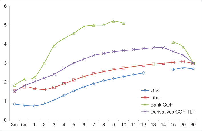
Figure 10.24 Derivatives funding curve as secured funding COF
The above of course is in the “wholesale” or investment bank space. In reality, derivatives dealers are often part of “universal” banking groups that also include retail and corporate business lines. A large part of the balance sheet will be funded therefore by low‐cost liabilities of contractual short‐dated but behaviourally long‐dated maturity. These also need to be factored into the pricing curve in a way that is appropriate. One approach might be to derive the derivatives COF off a “weighted average cost of funds” (WACF) curve that is an average of all balance sheet liabilities. Either way, care needs to be taken that business lines in the wholesale bank, which includes the derivatives desk, are charged an appropriate price and not necessarily the retail or corporate COF rate, particularly since customer deposits have short contractual tenors but long behavioural tenors, and so do not inflict a term liquidity premium (TLP) on the bank.
Derivative liabilities and assets
Derivative liabilities correspond to what is termed an overall expected negative exposure (ENE), the most basic example of which is a deposit. A derivative asset corresponds to an overall expected positive exposure or EPE and at its simplest would be a loan.
An appreciation of the terms of a derivatives funding policy requires an understanding of credit valuation adjustment (CVA), debt value adjustment (DVA), and funding value adjustment (FVA). Following existing literature (for example, see Picault (2005) and Gregory (2009)), under a set of simplifying assumptions we have:

where EPE is expected positive earnings, and PD and LGD are standard credit analyst expressions for default probability and loss given default. More formally we write:

where R is the recovery rate, q is the probability density function of counterparty default, and v is the value of the derivative payoff. In discrete time we write:

where qi is the probability of default between times ti‐1 and ti:
and
In other words, the discounting to be applied for valuation is at the appropriate tenor bank funding cost.
The funding cost to apply to the derivatives portfolio cash flows may sometimes be selected depending on what assumption we make about the ease of unwinding the portfolio:
- Assume no easy unwind: if we cannot unwind the portfolio without punitive costs, we must assume we will have to fund the transaction for the full term. The funding cost of this commitment is given by the bank's long‐term COF. If we fund (value) at short‐term COF we run the risk that sudden spikes in the short‐term COF will create funding losses, or that a liquidity squeeze in general will impact our ability to roll over funding for the position. To avoid this risk, we would fund with long‐term borrowing, and discount unsecured derivatives off the long‐term COF (TLP) curve;
- Assume easy unwind: if we can unwind the position with no extraneous cost, we can apply the short‐term COF, say the 1‐year TLP. The assumption of easy unwind means that we are not committed to rolling over funding; in the event of liquidity stress we would simply unwind the portfolio and eliminate the funding commitment. This is a strong assumption to make, particularly at a time of stress, and would be a high‐risk policy.
Therefore, in theory we recommend that the derivative asset be discounted at TLP and the funding for collateral postings be substantially term funded. That said, in some cases the funding generated from a derivative book (assuming no counterparty default) is contractually for a long maturity, and so the case may be made that this should be charged for or receive the secured funding rate as opposed to the unsecured COF rate. That being the case, the derivatives funding curve then sits below the bank's COF curve and closer to the secured funding curve. This is shown at Figure 10.24.
In general, when applying derivatives funding policy we assume no netting arrangements are in place, but in practice these are quite common and will have an impact on the bank's collateral funding position in the event of default.
Derivative portfolio maturity
The tenor period to apply when applying the correct funding cost to derivative book cash flows can be the contractual maturity of the derivative in question, but not necessarily so. An alternative approach is to split the portfolio into tenor buckets commensurate with the tenors at which we wish to fund the cash flows, with each bucket funded at the appropriate tenor COF.
Placing the derivative portfolio cash flows into appropriate term tenor buckets is a logical position on which to base how we choose to fund these cash flows. In practice, the derivative valuation model itself can be used to produce this tenor bucket breakdown, in the form of a “funding risk per basis point” (FR01) delta ladder. Using this model output removes the need for a subjective analysis of the maturity profile of the portfolio. In other words, the maturity profile of the portfolio is given by the model output. The appropriate tenor TLP is charged on the amount in each bucket.
This is shown at Figure 10.25.

Figure 10.25 Uncollateralised derivatives net position FTP pricing
In practice of course the profile is unlikely to look like the one in Figure 10.25 (although it might do). Rather, it is more likely to be all one way – either net long or short across most if not all tenor buckets.
In summary, cash flows arising out of the derivatives business, both contractual and collateral, must be funded at the appropriate TLP COF for their tenor. This means term funding a large part of the portfolio cash flows.
Funding valuation adjustment
Funding value adjustment is as important in derivative pricing as CVA, if not more so, and a vital part of an effective derivatives funding policy. When incorporating CVA, FVA, and where desired the cost of associated regulatory capital (“CRC”) into a transaction, we take a portfolio view with each individual counterparty. FVA represents the value adjustment made for the funding and liquidity cost of undertaking a derivative transaction.
To illustrate, consider a portfolio of just one plain vanilla IRS transaction. Assume it is fully collateralised with no threshold and daily cash collateral postings. This means that on a daily basis collateral is posted or received (MtM value). The bank exhibiting negative MtM borrows funds to post collateral at its unsecured COF, while collateral posted earns interest at the OIS rate (Fed Funds, SONIA, or EONIA). This is an asymmetric arrangement that impacts the pre‐crash norm of Libor‐based discounting of the IRS, which was acceptable when the bank was funding at Libor or at the inter‐bank swap curve. But post‐crash the higher bank COF means that funding adds to the cost of transacting the swap. The magnitude of this cost is a function of [OIS% – COF%] for the bank.
If we consider now a book of derivative transactions, the funding cost for the counterparty banks (“Banks A and B”) is a function of the size of the net MtM for the entire portfolio. Therefore, exactly as with CVA, to calculate the impact of the asymmetric funding cost we need to consider the complete portfolio value with each counterparty, as well as the terms of the specific CSA. This means in practice that when pricing the single swap, unless Banks A and B have the same funding costs – unlikely unless one is being very approximate – we see that the banks will not agree on a price for the instrument, irrespective of their counterparty risk and CVA.
That means a bank can choose to use FVA for a profitability‐type analysis only, not impacting swap MtM, or it can choose to cover this cost, in which case it will impact swap valuation. The decision may depend on the counterparty and the product/trade type, or it can be a universal one. But not passing it on or adjusting the price for FVA means the derivatives business line is not covering its costs correctly.
The position is not markedly different with uncollateralised derivatives, generally ones where one counterparty is a “customer”, for example, a corporate that is using the swap to hedge interest‐rate risk. The bank providing the swap will hedge this exposure with another bank, and this second swap will be traded under a CSA. This is shown in Figure 10.26.

Figure 10.26 Customer IRS and hedging IRS
The first swap has no collateral posting flows, but the second one does. This is in itself an asymmetric CSA position; moreover, the second swap cost will include an FVA element. The bank may wish to pass on this FVA hedge cost into the customer pricing, which means making the FVA adjustment to the swap price.
In both of the above illustrations, at any time the transaction (or hedge transaction) or portfolio MtM is negative, the bank will be borrowing cash to post as collateral. This borrowing is at the bank's cost of funds (COF), which we denote Libor + s where s is the funding spread. (Ignore specific tenor at this point.) If we look at FVA intuitively, it is an actual cost borne by the derivatives desk (and therefore the bank) as part of maintaining the derivatives portfolio – no different in cost terms than funding the cash asset side of the balance sheet. So at the very least, a bank needs to incorporate FVA into its derivatives business returns and profitability analysis. Ideally, the governance of FVA will be incorporated alongside all collateral management functions, including CVA, and overseen by the bank's Treasury/ALM function.
Notwithstanding the strategic objective of a balanced portfolio policy, the net impact of uncollateralised derivatives transactions or any asymmetric derivatives and hedging arrangement is to generate an ongoing unsecured funding requirement. We should expect this funding requirement to be in place as long as a bank is a going concern, in other words as ordinary business. Therefore, it should be funded in long‐term tenors, with only a minority proportion funded in short‐term tenors.
The cost of funding a derivatives portfolio, whether as a market‐maker or simply for hedging purposes, is an important part of the overall profitability of a bank and needs to be treated exactly as would the funding cost of a cash asset. FVA is one approach to measure funding cost. It can be passed on in customer pricing or the bank can choose to wear it, but the business line still needs to be charged for it (exactly as with cash asset funding).
The magnitude of FVA is a direct function of a bank's COF, which fluctuates, and so it is important for FVA to reflect current reality. By definition, banks with the highest COF (highest s and lowest perceived credit quality) will suffer a competitive disadvantage in this space.
Centralised clearing and ALM3
One of the policy decisions taken in the wake of the 2008 bank crash was the demand from regulators that hitherto “over‐the‐counter” (OTC) derivative transactions be settled, or “cleared”, through a centralised clearing counterparty (CCP), in the same way that exchange‐traded derivatives are settled at the clearing house. This would remove bilateral counterparty risk because every transaction participant would, in effect, be dealing with the clearing house. In theory, this removes counterparty credit risk, because the clearing house would be sufficiently collateralised so as never to go bankrupt.4
The role of CCP is being carried out by existing clearing houses such as London Clearing House in the European Union. While there are technical issues to consider when dealing in, say, USD IRS (because of the basis that exists between IRS cleared in the US and the EU), from an ALM perspective the issues that should be addressed may include:
- What price FVA to consider? The bank's TLP vs capital arbitrage;
- Who “owns” the collateral in the bank?;
- Impact on the Basel III NSFR liquidity requirement: all market participants will have to post a significant amount of “initial margin” with the CCP (or their agent bank). Thus, IM will act as a permanent drain of funding, with negative impact on the NSFR metric value;
- Optimising collateral (placing the cheapest available, in the cheapest currency, to the bank as collateral at the CCP);
- Impact on securities financing;
- The role of the XVA desk;
- Incentivising the right behaviour at business lines.
The collateral management impact of dealing via CCPs is considerable, and the orthodox treatment would be to place collateral management as a direct responsibility of the Treasury department.
Figure 10.27 (i) and (ii) summarise the key issues for consideration surrounding CCPs.
Figure 10.27 (i) Centralised clearing counterparty key points
Figure 10.27 (ii) Centralised clearing counterparty key points
CONCLUSIONS
Today the practice of liquidity risk management in banks is heavily prescribed by the regulatory regime in every jurisdiction. This was a natural response to the bank crash of 2008, and it places onerous requirements, in terms of resources and reporting, on all banks. As this chapter has shown, the liquidity risk discipline combines everything from cash management and funding to intra‐day liquidity and asset encumbrance. It is important that all banks have a deep and thorough understanding of all the drivers of liquidity risk exposure on the balance sheet, which is why the governance structure for liquidity management must run from ALCO downwards via Treasury. All aspects must be included (for example, traditionally collateral management was often placed in a back‐office operational function or outside Treasury: this would not be best practice today).
Liquidity risk management must remain the most important function in any bank at any time.