5

Demonstration of Meeting Needs: Verification and Validation

Recipes in this chapter

• Model simulation
• Model-based testing
• Computable constraint modeling
• Traceability
• Effective reviews and walkthroughs
• Managing model work items
• Test-driven modeling

George Box famously said that “all models are wrong, but some are useful,” (Box, G. E. P. (1976), “Science and statistics,” Journal of the American Statistical Association, 71 (356): 791–799). Although he was speaking of statistical models, the same can be said for MBSE models. In the systems world, models are both approximations of the real systems and subsets of their properties.

First, all models are abstractions; they focus on details of relevance of the system but completely ignore all other aspects. Therefore, the models are wrong because they don’t include all aspects of the system, just the ones we find of interest.

Second, all models are abstractions; they represent information at different levels of detail. When we model fluid flow in a water treatment system, we don’t model the interactions at the molecular level. Rather, we model fluid dynamics but not the interaction of electric fields of atoms bound together into molecules, let alone get into quantum physics. Therefore, the models are wrong, because they don’t model the electrodynamics of the particles and the interaction of the quantum fields of the elementary particles.

Third, all models are abstractions; they represent information at a level of precision that we think is adequate for the need. If we model the movement of an aircraft rudder control surface, we may very well decide that position, represented with 3 significant digits and an accuracy of ± 0.5 degrees, meets our needs. Therefore, our models are wrong because we don’t model infinite levels of precision.

You get the idea. Models are not exact replicas of reality. They are simplified characterizations that represent aspects in a (hopefully) useful conceptual framework with (also hopefully) enough precision to meet the need.

So, questions arise when considering a model:

1. Is the model right?
2. What does right mean?
3. How do we know?

We will try to provide some practical answers to these questions in this chapter. The answers will vary a bit depending on the kind of model being examined.

Let’s address the second question first: what does right mean? If we agree with the premise that all good models have a well-defined scope and purpose, then right surely means that it addresses that scope with the necessary precision and correctness to meet its purpose. If we look at a stakeholder requirements model, then the requirements it contains would clearly, unambiguously, and completely state the needs of the stakeholders with respect to the system being specified. If we develop an architecture, then the architectural structures it defines meet the system requirements and the needs of the stakeholder (or will, once it is developed) in an “optimal” way. If we develop a set of interfaces, then we describe all the important and relevant interactions with all the applicable details of that system with its actors.

If we use that answer for question #2, then the answer to the first question pertains to the veracity of the statement that the model at hand meets its scope and purpose. Subsequently, the answer to the third question is that we generate evidence that the answer to question #1 is, in fact, the case.

Verification and validation

Most engineers will agree with the general statement that verification means demonstration that a system meets its requirements while validation means demonstration that the system meets the need. In my consulting work, I take this slightly further (Figure 5.1):

Figure 5.1: Verification and validation core concepts

In my mind, there are two kinds of verification: syntactic and semantic. Syntactic verification is also known as compliance in form, because it seeks to demonstrate that the model is well-formed, not necessarily that it makes sense or represents statements of truth. This means that the model complies with the modeling language syntactic rules and the project modeling standards guidelines. These guidelines typically define how the model should be organized, what information it should contain, the naming conventions that are used, and action language used for primitive actions, and so on. Every project should have a modeling guidelines standard in place and it is against such a standard that the syntactic well-formedness of a model may be verified. See https://www.bruce-douglass.com/papers for downloadable examples of MBSE and MDD guidelines. In addition, check out SAIC’s downloadable style guide and model validation tool at.

Semantic verification is about demonstrating that the content makes sense; for this reason, it is also known as compliance in meaning. It is possible to have well-formed sentences that are either incorrect at best or nonsense at worst. There is even a Law of Douglass about this:

Any language rich enough to say something useful is also expressive enough to state utter nonsense that sounds, at first glance, reasonable.

Law of Douglass, #60

For the current state of the Laws of Douglass, see https://www.bruce-douglass.com/geekosphere.

The reason why this is important becomes clear when we look at the techniques of semantic verification (see Figure 5.1): semantic review, testing, and formal (mathematical) analysis.

If we have vague or imprecise models, we only have the first technique for ascertaining correctness: we can look at it. To be clear, a review is valuable and can provide insights for subtle issues or problems with a model; however, it is the weakest form of verification. The problem is largely one of vigilance. In my experience, humans are pretty good at finding issues for only a few hours at most before their ability to find problems degrades. You’ve probably had the experience of starting a review meeting with lots of energy but by the time the afternoon rolls around, you’re thinking, “Kill me now.” Reviews definitely add value in the verification process but they are insufficient by themselves. There’s a reason why we don’t say, “We can trust the million lines of code for the nuclear reactor because Joe looked at it really hard.”

The second technique for performing verification is to test it. Testing basically means that we identify a set of test cases – a set of inputs with specific values, sequence, and timing and well-defined expected outputs or outcomes – and then apply them to the system of interest to see if it performs as expected. A test objective is what you want to get from running the test case, such as the demonstration of compliance to a specific set of requirements. In SysML, a test case is a stereotype of behavior; in Cameo, a test case can be an activity, interaction, or state machine. This approach is more expensive than just looking at the system but yields far superior results, in terms of demonstration of correctness and identifying differences between what you want and what you have. Testing fundamentally requires executability and this is crucial in the MBSE domain. If we want to apply testing to our model – and we should – then it means that our models must be specified using a language that is inherently precise, use a method that supports executability, and use a tool environment that supports execution. An issue with testing is that it isn’t possible to fully test a system; there is always an essentially infinite set of combinations of inputs, values, sequences, and timings. You can get arbitrarily close to complete coverage at increasing levels of cost and effort, but you can never close the gap completely.

The third technique for verification is applying formal methods. This requires rendering the system in a mathematically precise language, such as Z or predicate logic, and then applying the rules of formal mathematics to demonstrate universals about the system. This is arguably the strongest form of verification but it suffers from two problems: 1. It is incredibly hard to do, in general. PhDs and lots of effort are required; and 2. The approach is sensitive to invariant violations. That means that the analysis must make some assumptions, such as “the power is always available” or “the user doesn’t do this stupid thing,” and if you violate those assumptions, you can’t trust the results. You can always incorporate any specific assumption in your analysis, but that just means there are other assumptions being made. Gödel was right (Kurt Gödel, 1931, “Über formal unentscheidbare Sätze der Principia Mathematica und verwandter Systeme,” I Monatshefte für Mathematik und Physik, v. 38 n. 1, pp. 173–198).

In my experience, the best approach for semantic verification is a combination of all three approaches – review, test, and analyze.

Verification is not the same as validation. Being valid means that the model reflects or meets the true needs of the stakeholders, even if those needs differ from what is stated in the system requirements. If meeting the system requirement is demonstrated through verification, meeting the stakeholder need is demonstrated through validation. For the most part, this is historically done with the creation of stakeholder requirements, and then reviewing the work products that describe the system. There are a couple of problems with that.

First, there is an “air gap” between complying with the stakeholder requirements and meeting the stakeholder need. Many a system has failed in its operational environment because, while it met the requirements, it didn’t meet the true needs. This is primarily why agile methods stress continuous customer involvement in the development process. If it can be discovered early that the requirements are not a true representation of the customer’s needs, then the development can be redirected and the requirements can be amended.

In traditional methods, customer involvement is limited to reviews of work products. In government programs, a System Requirements Review (SRR), Preliminary Design Review (PDR), and Critical Design Review (CDR) are common milestones to ensure the program is “on track.” These are almost always appraisals of many, many pages of description, with all of the problems inherent in the review previously mentioned. However, if you build executable models, then that execution – even if it is a simulated environment – can demonstrate how the system will operate in the stakeholders’ operational context and provide better information about system validity.

In this chapter, I will use the terms computable and executable when referring to well-formed models. When I say computable model, I mean a model that performs a computation, such as F=ma. In that equation, given two values, the system can compute the third, regardless of which two values are given. An executable model is a computable model in which the computation has a specific direction. Executable models are not necessarily computable. It is difficult to unscramble that egg or unexplode that bomb; these are inherently irreversible processes.

This chapter contains recipes that provide approaches to demonstrate the correctness of your models. We’ll talk about simulation when it comes to creating models, developing computational models for analysis, performing reviews, and creating system test cases for model verification.

Model simulation

When we test an aircraft design, one way is to build the aircraft and see if it falls out of the sky. In this section, I’m not referring to testing the final resulting system. Rather, I mean verifying the model of the system before detailed design, implementation, and manufacturing take place. SysML has some expressive views for representing and capturing structure and behavior. Both the IBM Rhapsody and No Magic Cameo SysML tools have some powerful features to execute and debug models as well as visualize and control that execution.

The Rhapsody modeling tool performs simulation by generating software source code from the model in well-defined ways, and automatically compiling and executing that code. Rhapsody can instrument this code to interact with the Rhapsody tool so that the tool can visualize the model execution graphically and provide control of the execution. This means that SysML models can be simulated, executed, and verified in a relatively straightforward fashion, even by non-programmers. Cameo, on the other hand, is a true simulation tool. It does not generate code for the execution of the simulation. While in many senses, the execution capabilities of Cameo are somewhat weaker than those in Rhapsody, the fact that Cameo provides a true simulation improves other capabilities. For example, because it performs simulation, Cameo gives you complete control over the flow of time, so time-based analyses are simplified in Cameo over Rhapsody.

Simulation can be applied to any model that has behavioral aspects. I commonly construct executable requirements models, something discussed in Chapter 2, System Specification. I do this one use case at a time, so that each use case has its own executable model stored in its own package. Architectural models can be executed as well to demonstrate their compliance with the use case models or to verify architectural specifications. Any SysML model or model subset can be executed if it can be specified using well-define behavioral semantics and is rendered in a tool that supports execution.

Purpose

The purpose of a model simulation is to explore, understand or verify the behavior of a set of elements defined within the model. This simulation can be used to evaluate the correctness of a model, to explore what-if cases, or to understand how elements collaborate within a context.

Inputs and preconditions

The model is defined with a purpose and scope, and a need for simulation has been identified.

Outputs and postconditions

The results of the simulation are the computation results of running the simulation. These can be captured in values stored in the model, as captured diagrams (such as animated sequence diagrams), or as outputs and outcomes produced by the simulation.

How to do it

Figure 5.2 shows the workflow for performing general-purpose model-based simulation. Given the powerful modeling environment, it is generally straightforward to do, provided that you adhere to the tooling constraints:

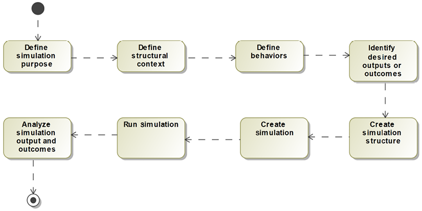
Figure 5.2: Model simulation workflow

It is common to have many different simulations within a systems model, to achieve different purposes and results. In Cameo, a simulation context is normally a block – it defines the set of elements (as parts) that collaborate in the simulation.

You may also create a simulation configuration with properties such as listeners, including sequence diagrams and user interfaces, as defined within the Cameo tool. It is common to have many such structures within a single MBSE model.

Define simulation purpose

It is imperative that you understand why you’re performing model simulation in order to get a useful outcome. I like to phrase the problems as “what does success smell like” in order to ensure that you’re going after the kind of results that will address your concerns. It matters because the models you create will vary depending on what you want to achieve.

Common purposes of model simulation include:

• Ensure the completeness and correctness of a set of requirements traced to by a use case.
• Demonstrate the adequacy of a set of interfaces.
• Explore behavioral options for some parts of a design model.
• Prove compliance of an architecture with a set of requirements.
• Reveal emergent behaviors and properties of a complex design.
• Verify a system specification.
• Validate a system architecture.
• Explore the consequences of various input values, timing, and sequence variation (“what-if” analyses).

Define structural context

The structural context for the model identifies the structural elements that will exhibit behavior – or used by structural elements that do – during the simulation. This includes blocks, use cases, and actors, along with their structural properties, such as value and flow properties, ports, and the relations among the structural elements.

Define behaviors

At the high-level, behavioral specification such as activity and state models provide the behavior of the system context as a whole or of the individual structural elements. At the detailed level, operations and activities specify primitive behavioral elements, often expressed in an action language, such as C, C++, Java, or Ada. In Cameo, I use the Groovy language, even though the default action language is, inexplicably, English. I can find and download a language specification for Groovy but not, again inexplicably, for Cameo’s English usage.

It should be noted that the SysML views that contribute directly to the simulation and code generation are the activity and state diagrams, and any code snippets put into the action and operation definitions. Sequence diagrams, being only partially constructive, do not generally completely specify behavior; rather, they depict specific examples of it, although in Cameo, they can be used to drive a simulation.

Identify desired outputs or outcomes

In line with the identification of the simulation purpose, it is important to specify what kind of output or outcome is desired. This might be a set of output interactions demonstrating correctness, captured as a set of automatically generated sequences (so-called “animated sequence diagrams”). Or it might be a demonstration that an output computation is correct under different conditions. It might even be “see what happens when I do this”. Clarity in expectation yields satisfaction in outcomes.

Define simulation structure

The simulation structure refers to the elements used to create the simulation. In Cameo, this will be the set of elements that participate in the simulation, a simulation context (typically a block), and, optionally, a simulation configuration and user interface.

Create simulation

Creating the simulation is easily done by right-clicking the simulation context and selecting Simulation > Run, or selecting the simulation configuration in the simulation configuration selection list. In Cameo, it’s common to create a diagram that contains other diagrams and use this to visualize the behaviors of the simulation. While this can be almost any kind of diagram, I generally use a BDD or free-form diagram. Cameo has properties that can be specified for simulation initialization in the Options > Environment > Simulation menu. See a description of these options at https://docs.nomagic.com/display/CST185/Automatic+initialization+of+context+and+runtime+objects.

Run the simulation

Once created, the executable can be run as many times and under as many different circumstances as you desire. In Cameo, ill-formed models are detected either by running validation checks (with Analyze > Validation > Validate) or through execution. When a problem occurs during the execution, the element manifesting the problem will drop out of the simulation and an obscure error message is displayed.

Analyze simulation outputs and outcomes

The point of running a simulation is to create some output or outcome. Once this is done, it can be examined to see what conclusions can be drawn. Are the requirements complete? Were the interfaces adequate? Did the architecture perform as expected? What behavior emerged under the examined conditions? I especially like creating animated sequence diagrams from the execution for this purpose.

Example

The Pegasus model offers many opportunities to perform valuable simulations. In this case, we’ll simulate one of the use cases from Chapter 2, System Specification, Emulate Basic Gearing. The use case was used as an example to illustrate the Functional analysis with scenarios recipe.

The mechanisms for defining simulations are tool-specific. The example here is simulated in Cameo and uses the Groovy action language. If you’re using a different SysML tool, then the exact means for defining and executing your model will be different.

Define simulation purpose

The purpose of this simulation is to identify mistakes or gaps in the requirements represented by the use case.

Define structural context

The execution context for the simulation is shown in Chapter 2, System Specification, in Figure 2.9 and Figure 2.10. The latter is an internal block diagram showing the connected instances of the actor blocks prtTrainingApp:aEBG_TrainingApp and prtRider:aEBG_Rider and the instance of the use case block itsUc_EmulatedBasicGearing:Uc:EmulateBasicGearing.

This model uses the canonical model organization structure identified in the Organizing your models recipe from Chapter 1, Basics of Agile Systems Modeling (see Figure 1.35). In line with this recipe, the detailed organization of the model is shown in Figure 5.3:

Figure 5.3: Organization of simulation elements

The Functional Analysis Pkg package contains a package for every use case being analyzed. This figure uses arrows to highlight elements and packages of importance for the simulation, including the actor blocks, the Events Pkg package, the Sim Support Pkg package, and the use case block. The Sim Support Pkg package contains the simulation configuration and UI developed for the simulation.

Define behaviors

The use case block state machine is shown in Figure 2.11. This state machine specifies the behavior of the system while executing that use case. The state machine represents a concise and executable restatement of the requirements and is not a specification of the design of the system. Figures 2.12 and Figure 2.13 show the state machines for the actor blocks. Elaborating the behavior of the actors for the purpose of supporting simulation is known as instrumenting the actors. Actor instrumentation is non-normative (since the actors are external to our system and we’re not designing them) and is only done to facilitate simulation.

Identify desired outputs or outcomes

The desired outcome is to either identify missing requirements by applying different test cases to the execution, or to demonstrate that the requirements, as represented by the model, are adequate. To do this, we will generate animated sequence diagrams of different situations, examine the captured sequences, and validate with the customer that it meets the need. We will also want to monitor the output values to ensure that the Rider inputs are processed properly and that the correct information is sent to the Training App. Note that this is a low-fidelity simulation and doesn’t emulate all the physics necessary to convert input Rider torque and cadence into output resistance and take into account Rider weight, wind resistance, current speed, and incline. While that would be an interesting simulation, that is not our purpose here.

We want to ensure that the Rider can downshift and upshift within the gearing limits, and this results in changing the internal gearing and the Training App being notified. Further, as the Rider applies input power, the output torque should change; a bigger gear with the same input power should result in larger output torque. These relations are built into the model; applied torque and resistance are modeled as flow properties while upshift and downshift are simulated with increment gear and decrement gear signal events. Further, the gearing (represented in gear inches, which is the distance the bike travels with one revolution of the pedal) should be limited between a minimum of 30 and a maximum of 140, while a gear shift changes the gearing by a constant 5 gear inches, up or down.

For this simulation, the conditions we would evaluate include:

• The gearing is properly increased as we upshift.
• The gearing no longer increases if we try to upshift past the maximum gearing.
• The gearing is properly decreased as we downshift.
• The gearing no longer decreases if we try to downshift past the minimum gearing.
• For a given level of input force, the output resistance is increased as we upshift (although the correctness of the output resistance is not a concern here).
• For a given level of input force, the output resistance is decreased as we downshift (although the correctness of the output resistance is not a concern here).

Define simulation view

Another nested package, named Sim Support Pkg, contains three things of interest with regard to the simulation structure. First, it contains a simulation configuration. In this case, the execution target is the context of the simulation, the block Emulate Basic Gearing Context. It also specifies that there is an execution listener, a Sequence Diagram Generator Config. Using this listener means that when the simulation is performed, an animated sequence diagram is created.

In addition, a UI Frame is added. This user interface allows the simulator to insert events and monitor and control values within the running simulation. The UI Frame is set to be the UI for the simulation configuration. See Figure 5.4:

Figure 5.4: Simulation Settings

Although not a part of the simulation structure per se, the figure shows a simple panel used to visualize and input values and to enter events during the execution. Such UI Frames are not the only means Cameo provides to do this, but they are convenient.

Create simulation

Creating the simulation is a simple matter of selecting the simulation configuration to run from the simulation configuration list, and clicking the Play button. This list is directly beneath the Analyze menu at the top of the Cameo window.

Run the simulation

Simply run the simulation configuration. With a simulation configuration being run, the simulation starts immediately. If you simulate by right-clicking on a block, there is an extra step of clicking a green triangle on the Simulation Toolkit window that pops up. In this case, the start of the simulation looks like Figure 5.5:

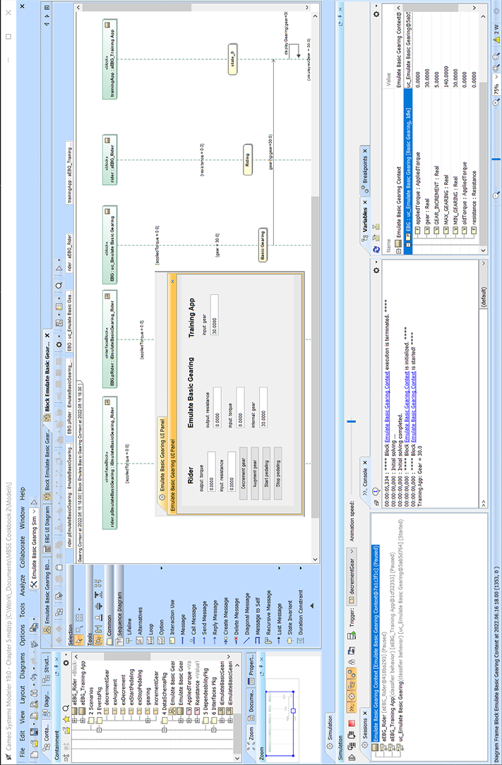
Figure 5.5: Running the simulation

Analyze simulation outputs and outcomes

We capture the inputs and outputs using a number of simulation runs. In the first such run, we initialize the running simulation to output a resistance of 100 and the rider to provide a power value of 200. Then we augment the gearing and see that it increases. Further, the training app is updated with the gearing as it changes. We see that in the animated sequence diagram in Figure 5.6:

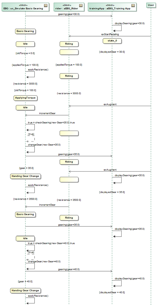
Figure 5.6: Simulation run 1

Since the system starts in the lowest gear, the next simulation run should demonstrate that an attempt to downshift below the minimum gearing should result in no change.

That’s what we see in Figure 5.7; notice the coloring of the animated state machine shows the [else] path was taken and the gearing was not decremented. This is also seen in the gear value for the Emulate Basic Gearing panel (highlighted with arrows). The sequence diagram shows the false result of the guard following the exDecrement signal event:

Figure 5.7: Simulation run 2

In the last run shown here, we set the gearing to 135, and then augment it twice to try to exceed the maximum gearing of 140 gear inches. We should see the resistance value go up with the first upshift, and then not change with the second. This is in fact what we see in Figure 5.8.

I’ve marked relevant points in the figure with red arrows. In the state diagram, you can see the [else] path was taken because the guard correctly identifies that the gear is at its maximum (140 gear inches). You can see the value in the UI at the bottom left of the figure. The sequence diagram shows that the guard returns false and the limiting value, 140, is sent to the Training App:

Figure 5.8: Simulation run 3

We have achieved the desired outcome of the simulation by demonstrating that the requirements model correctly shifts up and down, stays within gearing limits, properly updates the output resistance as the gearing is changed, and the Training App is properly notified of the current gearing when it changes.

Model-based testing

If you agree that modeling brings value to engineering, then Model-Based Testing (MBT) brings similar value to verification. To be clear, MBT doesn’t limit itself to the testing of models. Rather, MBT is about using models to capture, manage, and apply test cases to a system, whether or not that system is model-based. In essence, MBT allows you to:

• Define a test architecture, including:
  • Test context
  • Test configuration
  • Test components
  • The System Under Test (SUT)
  • Arbiter
  • Scheduler
• Test cases, using:
  • Sequence diagrams (most common)
  • Activity diagrams
  • State machines
  • Code
• Test objectives

Bringing the power of the model to bear on the problems of developing test architectures, defining test cases, and then performing the testing is compelling. This is especially true when applying it in a tool like Cameo that provides such strong simulation and execution facilities.

While MBT can be informally applied, the UML Testing Profile specifies a standard approach. The profile defines a standard way to model test concepts in UML (and therefore in SysML). Figure 5.9 shows the basic meta-architecture of the profile.

While it doesn’t exactly represent what’s in the profile, I believe it explains it a little better.

Figure 5.9: UML Testing Profile meta-architecture

I don’t want to spend too much time on the details of the profile definition; interested people can check out the standard itself (https://www.omg.org/spec/UTP2/2.1/PDF) or books on the topic such as Model-Driven Testing (https://www.amazon.com/Model-Driven-Testing-Using-UML-Profile/dp/3540725628/ref=sr_1_1?dchild=1&keywords=uml+testing+profile&qid=1606409327&sr=8-1) by Baker, et al. However, I do want to highlight some aspects.

First, note that a Test Case is a stereotype of UML’s metaclass Behavior such as an interaction, activity, or state machine. That means we can define a Test Case using the standard SysML behavioral representations.

The Test Context includes a set of Test Cases, and also a set (one or more) of SUTs. The SUT is a kind of Classifier, from the UML Metamodel; Classifiers can be Blocks, Use Cases, and Actors (among other things of course), which can be used in a context as singular design elements, composite elements such as subsystems, systems, or even an entire system context. SUTs themselves can, of course, have behavior. The Test Log records the executions of Test Cases, each of which includes a Verdict, of an enumerated type.

You can model these things directly in your model and build up your own Test Context, Test Cases, and so on. Cameo provides an implementation of the Testing Profile, which can be installed in the Help > Resource/Plugin Manager dialog, which we will use in the recipe.

Purpose

The purpose of model-based testing is to verify the semantic correctness of a system under test by applying a set of test cases. This purpose includes the definition of the test architecture, the specification of the test cases, the generation of the outcomes, and the analysis of the verdict – all in a model-based fashion.

Inputs and preconditions

The preconditions include both a set of requirements and a system that purports to meet those requirements. The system may be a model of the system – such as a requirement or design model – or it may be the final delivered system.

Outputs and postconditions

The primary output of the recipe is a test log of a set of test executions, complete with pass/fail verdicts of success.

How to do it

A model-based test flow (Figure 5.10) is pretty much the same as a normal test flow but the implementation steps are a bit different:

Figure 5.10: Model-based test workflow

Identify system under test

The SUT is the system or system subset that we want to verify. This can be a use case functional analysis model, an architecture, a design, or an actual manufactured system. If it is a design, the SUT can include a single design element or a coherent set of collaborating design elements.

Define test architecture

The test architecture includes, at a minimum, the instance of the SUT and test components substituting for elements in the actual environment (“test stubs”). The test architecture can also include a test context (a test manager), scheduler, and arbiter (to determine verdicts).

Specify test cases

Before we start rendering the test cases themselves, it makes sense to specify the test cases. The test cases include the events the test architecture will introduce and include the values of data they will carry, their sequence and timing, and the expected output or outcome.

Relate test cases to requirements

I am a huge fan of requirements-based testing. I believe that all tests should ultimately be trying to verify the system against one or more requirements. This step in the recipe identifies one or more test cases for each requirement of the SUT. In the end, there should be no requirements that are not verified by at least one test case, and there are no test cases for which there are no requirements.

Analyze test coverage

Test coverage is a deep topic that is well beyond the scope of this book. However, we will at least mention that coverage is important. Test coverage may be thought of in terms of the coverage of the specification (need) and coverage of the design (implementation). In terms of coverage of the specification we can think in terms of coverage of the inputs (sources and events types, values, value fidelity, sequences, and timings) and outputs (targets and event types, values, sequences, accuracy, and timings).

Design coverage is different. Mostly, it is evaluated in terms of path coverage. This is best developed in safety-critical software testing standards, such as DO-178 (https://my.rtca.org/NC__Product?id=a1B36000001IcmwEAC or see https://en.wikipedia.org/wiki/DO-178C for a discussion of the standard), that talk about three levels of coverage:

• Statement coverage: every statement should be executed in at least one test case.
• Decision coverage: statement coverage plus each decision point branch should be taken.
• Modified condition/decision coverage (MC/DC):
  • Each entry and exit point is invoked.
  • Each decision takes every possible outcome.
  • Each condition in a decision is evaluated in every possible outcome.
  • Each condition in a decision is independently evaluated as to how it affects the decision outcome.

The point of the step is to ensure the adequacy of the testing given the set of requirements and the structure of the design.

Render test cases

In model-based testing, we have a number of options for test specifications. The most common is to use sequence diagrams; since they are partially constructive, they are naturally suited to specify alternative interaction flows. The second most common approach is to specify multiple test paths using activity diagrams. The third is to specify the test cases with a state machine, a personal favorite. You can always write scripts (code) for the test cases, but as that isn’t very model-based, we won’t consider it here.

Apply test cases

The stage (test architecture) is set and the dialog (the test cases) has been written. Now comes the performance (test execution). In this step, the test cases are applied against the SUT in the context of the text architecture. The outcome of each test case is recorded in the test log along with a pass or fail verdict.

Render verdict

The overall verdict is a roll-up of the verdicts of the individual test cases. In general, an SUT is considered to pass the test only when it passes all of the test cases.

Fix defects in SUT

If some test cases fail, that means that the SUT didn’t generate the expected output or outcome. This can be either because the SUT, the test case, or the test architecture is in error. Before moving on, the defect should be fixed and the tests rerun. In some cases, it may be permissible to continue if only non-critical tests fail. When I run agile projects, the basic rule is that critical defects must be addressed before the iteration can be accepted, but non-critical defects are put into the backlog for a future iteration and the iteration can progress.

To classifiy a defect as “critical” in this context, I generally use the severity of the consequence as the deciding factor. If the defect could have a significant negative outcome, then it is critical; such outcomes include system crashing or enable an incorrect decision or output that would have grave impact on system use. Causing a patient to die or leading a physician to a misdiagnosis of a medical issue would be a critical defect; having the color of an icon the wrong shade of red would not be.

Example

In this example, we’ll look at the portion of the architectural design of the Pegasus system that accepts inputs from the Rider to change gears and make sure that the gears are properly changed within the Main Computing Platform.

To simplify the example, we won’t look at the impact changing gears has on the delivered resistance.

Identify system under test

The system under design includes a few subsystems and some internal design elements. We are limiting ourselves to only designing the part of the system related to the rider’s control of the gearing within those design elements. To show the element under test will take a few diagrams, so bear with me:

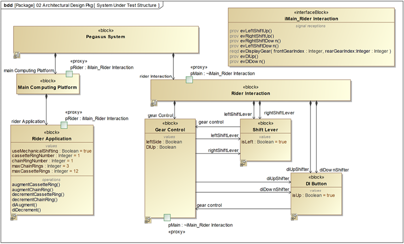
Figure 5.11: SUT structure

Figure 5.11 shows the blocks that together constitute the SUT: the Rider Interaction subsystem, which internally contains left and right Shift Levers and up and down Digital Indexed (DI) shift buttons (DI Button), is one key part. The other key part is the Main Computing Platform, which contains the Rider Application that manages the gears. This diagram shows the blocks and their relevant properties.

This diagram doesn’t depict well the runtime connected structure, so another diagram, Figure 5.12, shows how the instances connect:

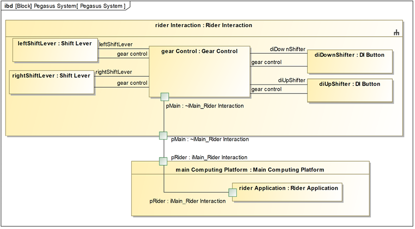
Figure 5.12: Connected parts in the SUT

All of these blocks have state machines that specify their behavior. The DI Button has the simplest state machine, as can be seen in Figure 5.13. As the Rider presses the DI Button, it sends an evDIShift event to the Gearing Control instance. The event carries a Boolean parameter that specifies it is the up (TRUE) or down (FALSE) button. The Gearing Control block initializes one of the DI buttons to be the up button and one to be the down button:

Figure 5.13: DI Button state machine

The Shift Lever state machine is only a little more complicated (Figure 5.14). The left Shift Lever controls the front chain ring and can either augment or decrement it; the right Shift Lever controls the cassette ring gear but works similarly. The state machine shows that either shift lever can send the evShiftUp or evShiftDown event. As with the evDIShift event, these events also carry a parameter that identifies which lever (left (true) or right (false)) is sending the event:

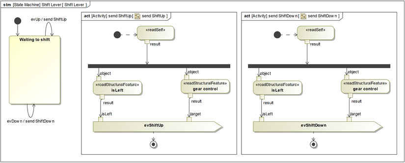
Figure 5.14: Shift Lever state machine

The Gear Control state machine is more complex, as you can see in Figure 5.15. It receives events from the left and right Shift Levers and the up and down DI Buttons. It must use the passed parameters to determine which events to send to the Rider Application. It does this by assigning a value property to be the passed parameter (either leftSide or DIUp, depending on which event), and then uses that value in a guard.

The lower AND-state handles the display of the current gearing confirmed by the Rider Application; this is sent by the Rider Application after it adjusts to the selected gears.

Also notice the initialization actions on the initial transition from the Initializing to the Controlling Gears state; this specifies the handedness of the Shift Levers and the DI Buttons:

Figure 5.15: Gear Control state machine

The last state machine, shown in Figure 5.16, is for the Rider Application, which is owned by the Main Computing Platform subsystem. This state machine supports both mechanical shifting and DI shifting. It works by receiving the events from the Gear Control block and augments/decrements the gearing based on the values:

Figure 5.16: Rider Application state machine for gearing

The gear adjustments are made by operations that ensure that the gearing remains within the set limits (1 to maxChainRings and 1 to maxCassetteRings). Figure 5.17 shows a table of the opaque behaviors (code snippets) for each of the operations referenced in Figure 5.16. Note that the operation itself is in the Specification column.

The methods are all written using the Groovy language:

Figure 5.17: Functions for setting gearing

Finally, the request display act behavior invoked on the Rider Application state machine is shown in Figure 5.18:

Figure 5.18: Request display act

So, there’s our system under test. Is it right? How can you tell? Without testing, it would be easy for simple mistakes to creep in.

Define test architecture

The test architecture includes the development of the test fixtures or stubs we will use to perform the test. The test fixtures must provide the ability to repeatably set up the initial starting conditions for our tests, introduce the events with the proper values, sequences, and timings, and observe the results and outcomes.

We could create some blocks to do this in an automatic fashion. I personally use the stereotypes «testbuddy» and «testarchitecture» for such created elements.

Figure 5.19: Pegasus test architecture

Figure 5.19 shows the Test Context block added with the SUT, Pegasus System, as a part. This means that the testing doesn’t interfere at all with the behavior or structure of the SUT. It is, of course, important to not modify the elements of the SUT for the purpose of the test, as much as possible. As the testing maxim goes, “Test what you do; do what you test.” In this case, no modifications of the SUT to facilitate testing are necessary. Sometimes you may want to add «friend» relations from the elements of the SUT to the test components to make it easier to perform the tests. Note that the Test Context block has value properties of type VerdictKind from the SysML profile or Verdict from the testing profile. These will hold the outcomes of the different test cases (in this case, test # 1, 3, 7, and 9). We will capture the outcomes of the test runs as instance specifications of type Test Context to record the outcomes.

There are many approaches to doing a model-based test, but in this example, we will use elements from the Cameo Testing Profile plugin.

Specify test cases

Let’s think about the test cases we want (Table 5.1). This table describes the test cases we want to apply:

Table 5.1: Test case descriptions

To fully test with even the limited functionality we’re looking at, more test cases are needed, but we’ll leave those as exercises for you. This should certainly be enough to give the reader a flavor of model-based testing.

Relate test cases to requirements

To look at how the tests address the requirements, I created «verify» relations from each of the test cases to the set of requirements they purported to verify. I then created a matrix displaying those relations. Obviously, more test cases are needed, but Figure 5.20 shows the starting point for test case elaboration:

`

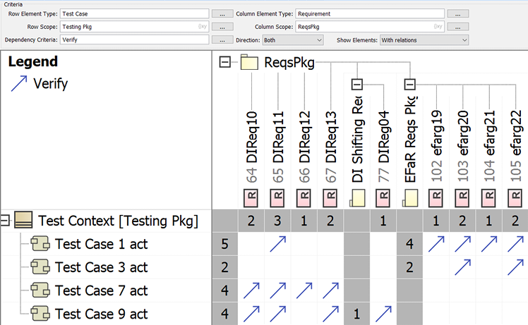
Figure 5.20: Test case verifies requirements table

Analyze test coverage

For our purposes here, we will examine coverage in terms of both the requirements and path coverage in the SysML behavioral models – that is, our test cases should execute every transition in each state machine and every control flow in every activity diagram.

As far as requirements coverage, there is a test case for the requirements in Figure 5.20, but many more requirements are not yet covered. We must also consider the degree completion of the coverage of requirements that are covered. The control of the chain ring in mechanical shifting mode is pretty complete: we have test cases to ensure that in the middle of the range, augmenting and decrementing work properly, that you can’t augment beyond the limit, and that you can’t decrement below the minimum. However, what about DI mode? There are a couple of test cases but we should consider cases where augmentation forces a change in the chain ring as well as the cassette ring, where gear decrement forces a reduction in the chain ring, and cases where they can be handled completely by changing the cassette ring only. In addition, we need cases to ensure that the calculations are right for different gearing configurations, and that we can’t augment or decrement beyond available gearing.

To consider design coverage, you can “color” the transitions or control flows that are executed during the executions of tests. As more tests are completed, fewer of the transitions in the design element state behaviors should remain uncolored. One nice thing about the Cameo Simulation Toolkit is that it does color states, actions, transitions, and control flows that are executed, so it is possible to visually inspect the model after a test run.

Render test cases

We will implement these case cases with activity behavior in the Test Context block. The testing profile defines Behavior and Operation as the base metaclasses for the «testcase» stereotype; I’ve applied that stereotype to those specific testing activities. One result of doing this is that each test case has an output activity parameter named verdict, which is of enumerated type VerdictKind. The potential values here are pass, fail, inconclusive, or unknown. The basic structure of this test suite is shown in Figure 5.21.

The Test Context behavior runs the four rendered tests in order; in each case, the initial starting conditions for the test are set, and then the test is run:

Figure 5.21: Test architecture main behavior

To assist in the execution of the test cases, I also created a simulation configuration. In the configuration, I set the run speed to 100% and instructed the system to put the final resulting instance in the Testing Results package. This allows me to create an instance table of test case runs:

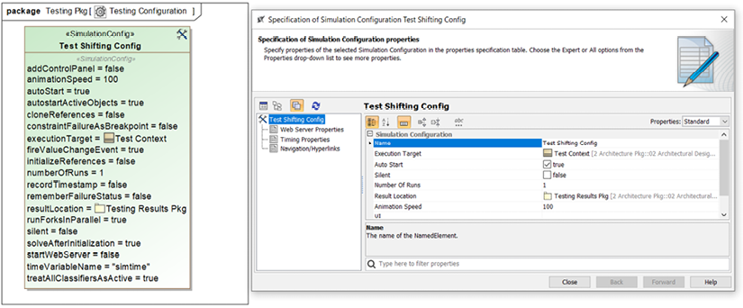
Figure 5.22: Test simulation configuration

Let’s render just four of these test cases: 1, 3, 7, and 9.

Render test case 1: Augment the front chain ring from 1 to maxChainRings (3).

Adding the state behavior for this test case is pretty simple. The initialization just needs to:

• Set the shifting mode to mechanical shifting.
• Set the selected chain ring to the first (1).

The test execution behavior is pretty simple. The system just needs to send the left Shift Lever the evUp event and verify that both the set chain ring and the displayed chain ring are correct. Figure 5.23 shows the details of the state TC1_Execution activity:

Figure 5.23: Test case 1 specification

In this case, test case 1 sends the leftShiftLever part the signal evUp. Following a short delay to allow the target to receive and consume the incoming signal, the values of the cassetteRingNumber and chainRingNumber are checked, and if found to be correct, the test case returns a verdict of pass; otherwise, it returns a verdict of fail.

Render test case 3: Augment chain ring out of range high

In this test case, the set up for the test for mechanical shifting and sets the selected chain ring to 3. It tries to augment the chain ring (which is already at its maximum); it should remain at the value 3.

The test case activity is shown in Figure 5.24:

Figure 5.24: Test case 3 specification

Render test case 7: Move to DI shifting

This is an easy test case. All we have to do is to run the system and then check that the system is set to use DI shifting; this is best done by ensuring that the Gear Control state is currently DI Shifting. Cameo provides an action language helper named ALH.inState that returns a Boolean if the specified instance is in the specified state and False otherwise.

The activity for test case 7 is shown in Figure 5.25:

Figure 5.25: Test case 7 specification

Render test case 9: With DI shifting, press UP three times to see that shifting works

In the last test case, we’ll enter DI mode and then shift UP twice to ensure that shifting works. The gearing is initialized to chain ring 1 and cassette ring 2 with DI shifting enabled. The test presses the DI Up Button three times, and we expect to see it augment the gearing to 1:2 and on to 1:3:

Figure 5.26: Test case 9 specification

Apply test cases

Now, let’s run the test cases and look at the outcomes. Since I think you learn more from test failures than successes, prepare to see some failures. In the Test Results Pkg package, I added an instance table showing the results generated by running the test case. In it, we can see that while test 1 passed, test cases 3, 7, and 9 failed:

Figure 5.27: Test results instance table

Render verdict

As not all tests succeeded, the test suite, as a whole, fails. This means that the design must be repaired and the tests rerun.

Fix defects in SUT

The defects are all fairly easy to fix. For test 3, the issue is in the implementation of the Rider Application operation augmentChainRing. The current implementation is:

if (chainRingNumber <= maxChainRings) chainRingNumber++;

but it should be:

if (chainRingNumber < maxChainRings) chainRingNumber++;

Tests 7 and 9 failed because the Rider Application activity send DI Shifting act sent the wrong event. In Figure 5.16, you can see that it sends the evMechanicalShifting event, but it should send the evDIShifting event. This is fixed in the following diagram:

Figure 5.28: Updated Rider Application behavior

After making the fixes, we can rerun the test suite. We can see in Figure 5.29 that all the tests pass in the second run:

Figure 5.29: Test outcomes take two

Computable constraint modeling

Mathematics isn’t just fun; it’s also another means by which you can verify aspects of systems. For example, in the Architectural trade studies recipe in Chapter 3, Developing System Architecture, we created a mathematical model to evaluate design alternatives as a set of equations, converting raw properties – including measurement accuracy, mass, reliability, parts cost and rider feel – into a computed “goodness” metric for the purpose of comparison. Using trade studies is a way to verify that good design choices were made. We did this using SysML constraints and parametric diagrams to render the problem and “do the math.”

Math can address many problems that come up in engineering, and SysML parametric diagrams provide a good way to render, compute, and resolve such problems and their solutions. An archetypal example is computing the total weight of a system. This can be done by simply summing up the weights of all its constituent parts. However, far more interesting problems can be addressed.

Because math is the language of quantities, it is very general, so it is a challenge to come up with a workflow that encompasses a wide range of addressable problems. But we are not alone. Thinkers such as Polya (Polya, G. How to Solve It: A new aspect of mathematical methods, Princeton University Press, 1945) or recent rereleases such as those available on Amazon.com and Wickelgren (Wickelgren, W. How to Solve Problems: Elements of a theory of problems and problem solving, W. H. Freeman and Co, 1974). have proposed means by which we can apply mathematics to general kinds of problems. As we did with in the trade studies, we can capture an approach that employs mathematics and SysML to provide a means to mathematically analyze and verify system aspects.

Purpose

The purpose is to solve a range of problems that can be cast as a set of equations relating to values of interest. We will call problems of this type Mathematically-Addressable Problems (MAPs).

Inputs and preconditions

The input to the recipe is a MAP that needs to be solved, such as the emergent properties of a system being developed.

Outputs and postconditions

The output of the recipe is the answer to the problem – typically, a quantified characterization of the emergent property (also known as the answer).

How to do it

Figure 5.30 shows the steps involved:

Figure 5.30: Computational constraint modeling workflow

Understand the problem

The first step in this recipe is to understand the problem at hand. In MBSE, that generally means:

• Identifying the structural elements (blocks, value properties, and so on).
• Discovering how they connect.
• Understanding how the elements behave both individually and collectively.
• Reviewing the qualities of services of those behaviors (such as worst-case performance).
• Looking at other quantifiable properties of interest for the system or its elements.

Identify the available truths

This step is about finding potentially relevant values and constraints. This might be universals – such as the value of the gravitational constant on the surface of the earth is 9.81 m/s² or that the value of π to nine digits is 3.14159265. It might be constraints – such as the limit on the range of patient weights (0.5 KG to 300 Kg). It might be quantifiable relations – such as F = ma.

Determine the necessary properties of acceptable solutions

This is the step where the problem gets interesting. I personally cast this as “what does the solution smell like?”. I want to understand what kind of thing I expect to see when a solution is revealed. Is it going to be the ratio of engine torque to engine mass? Is it the likelihood of a fault manifesting as an accident in my safety critical system? What is the nature of the result for which I am looking? Many times, this isn’t known or even obvious at the outset of the effort but is critical in identifying how to solve the problem.

Constrain the problem to only relevant information

Once we understand the problem, the set of potentially useful information, and the nature of the solution, we can often limit the input information to a smaller set of truly relevant data. By not having to consider extraneous information, we simplify the problem to be solved.

Construct the mathematical formulation

In this step, we develop the equations that represent the information and their relations in a formal, mathematical way. Remember, math is fun.

Render the problem as a set of connected constraint properties

The equations will be modeled as a set of constraints owned by SysML constraint blocks. The input and output values of those equations are modeled as constraint parameters. Then the equations are linked together into computation sets as constraint properties on a parametric diagram.

Perform analysis of units

In complex series of computations, it is easy to miss subtle problems that could be easily identified if you just ensure that the units match. Perhaps you end up trying to add inches to meters or add values of force and power. Keeping track of units and ensuring that they balance is a way to find such mistakes.

Do the math

Cameo can evaluate parametrics with its Simulation Toolkit. If you simulate a context that has parametrics, these are evaluated before the actual simulation begins in a pre-execution computational step.

Do a sanity check

A sanity check is a quick verification of the result by examining its reasonableness. One quick method that I often employ is to use “approximate computation.” For example, if you say that 1723/904 is 1.906, I might do a sanity check by noting that 1800/900 is 2, so the actual value should be a little less than 2.0. If you tell me that a medical ventilator should deliver 150 L/min, I might perform a sanity check by noting that an average breath is about 500 ml (at rest) at an average rate of around 10 breaths/min, so I would expect a medical ventilator to deliver something close to 5 L/min, far shy of the suggested value.

More elaborate checks can be done. For a critical value, you might compute it using an entirely different set of equations, or you might perform backward computation whereby you start with the end result and reverse the computations and see if you end up with the starting values.

Example

The Architectural trade studies recipe example from Chapter 3, Developing System Architectures, showed one use for computable constraint models. Let’s do another.

In this example, I want to verify a resulting computation performed by the Pegasus system, regarding simulated miles traveled as a function of gearing and cadence. We will build up and evaluate a SysML parameter model for this purpose.

Understand the problem

The potentially relevant properties of the Bike and Rider include:

• Chain ring gear, in the number of teeth.
• Cassette ring gear, in the number of teeth.
• Wheel circumference, inches.
• Cadence of the rider, in pedal revolutions per minute.
• Power produced by the rider, in watts.
• Weight of the rider and bike, in kilograms.
• Wind resistance of the rider, in Newtons.
• Incline of the road, in % grade.
• How long the rider rides, in hours.

The desired outcome is to know how far the simulated bike travels during the ride.

Identify the available truths

There are some constraints on the values these properties can achieve:

• Chain ring gears are limited to 28 to 60 teeth.
• Cassette ring gears are limited to 10 to 40 teeth.
• The wheel circumference for a normal road racing bike is 82.6 inches (2098 mm).
• Reasonable rider pedal cadence is between 40 and 120 RPM.
• Maximum output power for elite humans is about 2000W, with 150–400W sustainable for an hour or more (depending on the person).
• The UCI limits the weight of road racing bikes to no less than 15 lbs (6.8 Kg) but 17–20 lbs is more typical.
• Rider weight is generally between 100 to 300 lbs (45.3 Kg to 136 Kg).
• Wind resistance is a function of drag coefficient, cross-sectional area, and speed (https://ridefar.info/bike/cycling-speed/air-resistance-cyclist/).
• Road inclines can vary from -20 to +20% grade with an approximately normal distribution of around 0%. A notable exception is the 32% climb in the Savageman Triathlon “Westernport Wall,” https://kineticmultisports.com/races/savageman/.
• Ride lengths of interest are between 0.5 and 8 hours.

Determine the necessary properties of acceptable solutions

What we expect is a distance in miles as determined by a ride of a certain length of time in specific gearing, with other parameters being set as needed.

Constrain the problem to only relevant information

A little thought on the matter reveals that many of the properties outlined are not really relevant to the specific computation. Assuming no wheel slippage on the road, the only properties necessary to determine distance are:

• Chain ring gear
• Cassette ring gear
• Pedal cadence
• Wheel circumference
• Ride time

If the other properties vary, they will manifest as changing one or more of these values. For example, if wind resistance changes due to a headwind, then the rider will either pedal more slowly, change gear, or ride longer in time to cover the same distance.

Construct the mathematical formulation

There are a number of equations we must construct, with several of them solely for converting units:

• Gear ratio = chain ring teeth / cassette ring teeth.
• Gear inches = gear ratio * wheel circumference in inches.
• Gear miles = gear inches / 12 / 5280.
• Revolutions per hour = revolutions per minute * 60.
• Speed in MPH = revolutions per hour * gear miles.
• Distance = speed * duration.

Render the problem as a set of connected constraint properties

These equations are rendered as constraint blocks, as you can see in Figure 5.31. The inputs and outputs are shown as the constraint parameters, shown as included boxes along the edge of the constraint blocks.

The front gear and rear gear are modeled as Integers, but all others are represented as Reals:

Figure 5.31: Bike gear constraint blocks

A parametric diagram is a specialized form of an internal block diagram. The usage of the constraint blocks, known as constraint properties, in the computational context is shown in Figure 5.32:

Figure 5.32: Gear calculation parametric diagram

Note the binding connectors relate the constraint parameters together as well as the constraint parameters to the value properties of the Bike block. This will become important later in the recipe when we want to evaluate different cases.

Perform analysis of units

This problem is computationally simple but is easy to screw up because of the different units involved. Wheel circumference is measured in inches. Pedal cadence in RPM. However, we ultimately want to end up with the distance in miles.

We can recast the equations as units to ensure that we got the conversions right:

• Gear ratio = chain ring teeth / cassette ring teeth
  • Real = teeth / teeth (note: Real is unitless)
• Gear inches = gear ratio * wheel circumference
  • Inches / revolution = real * inches / revolution
• Gear miles = gear inches / 12 / 5280
  • miles / revolution = inches / revolution / (inches/foot) / (feet/mile)
  • = feet / revolution / (feet / mile)
  • = miles / revolution
• Revolutions per hour = revolutions per minute * 60
  • RPH = revolutions / min * (minute / hour)
  • = revolutions / hour
• Speed in MPH = revolutions per hour * gear miles
  • MPH = (revolutions / hour) * (miles / revolution)
  • = miles / hour
• Distance = speed * duration
  • Miles = miles / hour * hour
  • = miles

The units balance, so it seems that the equations are well-formed.

Do the math

Before we do the math, it will be useful to review SysML instance specifications a bit, as they are not covered in much detail in most SysML tutorials. An instance specification is the specification of an instance defined by a block. Instance specifications have slots that hold specific values related to the value properties of the block. That means we can assign specific values to the slots corresponding to value properties. In practice, we can assign a partial set of slot values and use the parametric diagram to compute the rest. We can then save the resulting elaborated instance specification as an evaluation case, much like we might have multiple parts instantiating a block. This concept is illustrated in Figure 5.33:

Figure 5.33: Blocks and instance specifications

To perform the math, we’ll define a set of instance specifications for the cases that we want to compute. In this example, we’ll look at six cases:

• 34 x 13 @ 90 RPM for 1 hour
• 34 x 18 @ 90 RPM for 1 hour
• 34 x 13 @ 105 RPM for 0.75 hour
• 53 x 13 @ 90 RPM for 1 hour
• 53 x 18 @ 90 RPM for 1 hour
• 53 x 13 @ 105 RPM for 1.5 hour

We will create a separate instance specification for each of these cases. Each of these cases is an instance specification typed by the block Bike. We will name these as “IS” + gearing + pedal cadence, such as IS 34x13 at 90 for 1 hour.

To perform the computations, we will use the Cameo Simulation Toolkit. This toolkit performs a pre-execution computation – that is, it evaluates the parameters in the simulation before performing any behaviors.

To actually perform the calculations is easy – if you know how (although it isn’t well explained in the documentation). Simply right-click on the Bike block and select Simulation > Run. Although the block has default values for the value properties, you can set the values that you want to compute for the different cases. Once completed, you can click the export to new instance button in the Simulation Toolkit (see Figure 5.34) to save the values as an instance specification. Select the package where you want the instance placed. You’ll have to rename it after it is created:

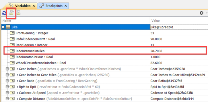
Figure 5.34: Simulation Toolkit variables window

I updated the computed properties and then constructed a table of the values for the different evaluation cases (Figure 5.35):

Figure 5.35: Instance table of computed outcomes

Do a sanity check

Are these values reasonable? As an experienced cyclist, I typically ride around 90 RPM, and in a gear 53x18 gear, I would expect to go about 20 miles, so the computed result for that case seems right. As I switch to a small 13-cog cassette, I would expect to go about 50% further, so the 28 miles at 53x13 seems about right. In a smaller front chain ring of 34 with a small cog (13), I’d expect to go about 80% as far as in the 53x18, so that seems reasonable as well.

Traceability

Traceability in a model means that it is possible to navigate among related elements, even if those elements are of different kinds or located in different packages. This is an important part of model verification because it enables you to ensure the consistency of information that may be represented in fundamentally different ways or different parts of the model. For example:

• Are the requirements properly represented in the use case functional analysis?
• Do the design elements properly satisfy the requirements?
• Is the design consistent with the architectural principles?
• Do the physical interfaces properly realize the logical interface definitions?

The value of traceability goes well beyond model verification. The primary reasons for providing traceability are to support:

• Impact analysis: determine the impact of change, such as:
  • If I change this requirement or this design element, what are the elements that are affected and must also be modified?
  • If I change this model element, what are the cost and effort required?
• Completeness assessment: how done am I?
  • Have I completed all the necessary aspects of the model to achieve its objectives, such as with a requirement, safety goal, or design specification?
  • Do I have an adequate set of test cases to verify the requirements?
• Design justification: why is this here?
  • Safety standards require that all design elements exist to meet requirements. This allows the evaluation of compliance with that objective.
• Consistency: are these things the same or do they work together? For example:
  • Are the requirements consistent with the safety concept?
  • Does the use case activity diagram properly refine the requirements?
  • Does the implementation meet the design?
• Compliance:
  • Does the model, or elements therein, comply with internal and external standards?
• Reviews:
  • In a review or inspection of some model aspect, is the set of information correct, complete, consistent, and well-formed?

By way of a very simple example, Figure 5.36 schematically shows how you use a trace matrix. The rows in the figure are the requirements and the columns are different design elements. Requirement R2 has no trace relation to a design element, indicating that is an unimplemented requirement. Conversely, design element D3 doesn’t realize any requirements, so it has no justification:

Figure 5.36: Traceability

Some definitions

Traceability means that a navigable relation exists between all related project data without regard to the data location in the model, its representation means, or its format.

Forward traceability means it is possible to navigate from data created earlier in the project to related data produced later. Common examples would be to trace from a requirement to a design, from a design to implementation code, or from a requirement to related test cases.

Backward traceability means it is possible to navigate from data created later in the project to related data produced earlier in the process. Common examples would be to trace from a design element to the requirements it satisfies, from a use case to the requirements that it refines, from code back to its design, or from a test case to the requirements it verifies.

Trace ownership refers to the ownership of the trace relation, as these relations are directional. This relation is almost always in the backward direction. For example, a design element owns the satisfy relation of the requirement. Forward traceability is supported by tools via automation and queries by looking at the backward trace links to identify their owners. This is counterintuitive to many people, but it makes sense. A requirement in principle shouldn’t know how it is implemented, but a design in principle needs to know what requirements it is satisfying. Therefore, the «satisfy» relation is owned by the design element and not the requirement.

Trace matrices are tabular relations of the relations between sets of elements. Cameo supports the creation of matrix layouts that define the kinds of elements for the rows and columns and the kind of relation depicted. Matrix views visualize data based on the layout specifications. Multiple kinds of relations can be visualized in the same matrix, but in general, I recommend different tables to visualize different kinds of trace links.

Types of trace links

In SysML, trace relations are all stereotypes of dependency. Table 5.2 shows the common relations in SysML:

Table 5.2: SysML trace relations

You may, of course, add your own relations by creating your own stereotype of dependency. I often use «represents» to trace between levels of abstraction; for example, a physical interface «represents» a logical interface.

It is reasonable to ask why there are different kinds of trace relations. From a theoretical standpoint, the different kinds of relation clarify the relation’s semantic intent. In practice, different tables can be constructed for the different kinds of relations and make them easier to apply in real projects.

Traceability and agile

Many Agilistas devalue traceability; for example, Scott Ambler says:

Too many projects are crushed by the overhead required to develop and maintain comprehensive documentation and traceability between it. Take an agile approach to documentation and keep it lean and effective. The most effective documentation is just barely good enough for the job at hand. By doing this, you can focus more of your energy on building working software, and isn’t that what you’re really being paid to do?

See http://www.agilemodeling.com/essays/agileRequirementsBestPractices.htm for more information.

However, in my books on agile systems engineering and agile development for real-time, safety-critical software, I make a case that traceability is both necessary and required:

Traceability is useful for both change impact analysis and to demonstrate that a system meets the requirements or that the test suite covers all the requirements. It is also useful to demonstrate that each design element is there to meet one or more requirements, something that is required by some safety standards, such as DO-178B.

See Bruce Douglass, Ph.D, Real-Time Agility (Addison-Wesley, 2009): https://www.amazon.com/Real-Time-Agility-Harmony-Embedded-Development/dp/0321545494 for more information.

In my agile projects, I add traceability relations as the work product content stabilizes to minimize rework, usually after most of the work has been done but before the system is verified and reviewed.

Purpose

The purpose of traceability is manifold, as stated earlier in this recipe. It enables model consistency and completeness verification as well as the performance of impact analysis. Additionally, it may be required by standards a project must meet.

Inputs and preconditions

The sets of elements being related are well enough developed to justify the effort to create trace relations.

Outputs and postconditions

Relations between related elements in different sets have been created and are captured in one or more trace matrices.

How to do it

Figure 5.37 shows the simple workflow for this recipe. Although the steps themselves are simple, not thinking deeply about the steps may result in unsatisfactory outcomes:

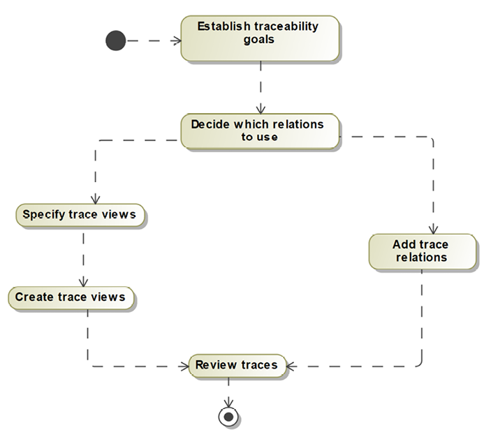
Figure 5.37: Create traceability

Establish traceability goals

Traceability can be done for a number of specific reasons. Different stakeholders care about demonstrating that the design meets the requirements, versus test cases adequately covering the design, versus ensuring that the stakeholder requirements are properly represented in the system requirements.

All of these are reasons to create traceability, but different trace views should be created for each purpose.

Common traceability goals in MBSE include tracing between:

• Stakeholder needs and system requirements.
• System and subsystem requirements.
• Subsystem requirements and safety goals.
• Facet (e.g., software or electronic) requirements and system requirements.
• Requirements and test cases.
• Design and test cases.
• Design and safety goals.
• Logical schemas and corresponding physical schemas, including:
  • Data schema
  • Interfaces
• Model products and standard objects, such as ASPICE, DO-178, and ISO26262.
• Design and implementation work products.

For your project, you must decide on the objectives you want to achieve with traceability. In general, you will create a separate traceability view for each trace goal.

Decide which relations to use

SysML has a number of different kinds of stereotyped dependency relations that can be used for traceability purposes. In modern modeling tools, you can easily create your own to meet any specified needs you have. For example, I frequently create a stereotype of dependency named «represents» to specifically address trace relations across abstraction levels, such as between physical and logical schemas.

Which relation you use is of secondary importance to establishing the relations themselves, but making good choices in the context of the set of traceability goals that are important to you can make the whole process easier. Table 5.3 shows how I commonly use the relations for traceability:

Table 5.3: Common trace relation usage

Specify trace views

Once the element type and relations are decided, you must decide the best way to represent them. The first decision here is whether to use a matrix or a table.

A matrix is often the first choice for traceability. A matrix is a relation table between element sets, one set shown in the rows and the other in the columns. The contents of the cells in the matrix indicate the presence or absence of the desired relation.

This is a great view for determining the presence or absence of relations. For example, the «satisfy» matrix between requirements and design elements is very useful to determine absence; an empty requirements row means that the requirement isn’t represented in the design while an empty design element column means that the design element isn’t there to meet any requirements. For practical reasons, I prefer the smaller set of elements to be shown as columns and the larger set of elements to be shown as the rows. The downside of a matrix is that you can’t see anything other than the name of the involved elements and the presence or absence of the desired relation. If you want to see other data, such as the text of the requirements, a list of the value properties of blocks, or the metadata tags, then a table is preferable.

Tables consist of rows of data, one per primary table element, along with information owned by or about that element about which you care. Table elements that have properties – such as textual specifications, value properties, or metadata held in owned tags – can display that data in an easy-to-read summary form. In the context of traceability, one of the kinds of properties the elements can own are relations, such as «trace» or «verify», and these can be shown in tables as well. In Cameo, this is done with the Columns tool above the table.

You can even create both tables and matrices.

Create trace views

Once the layouts are defined, create views that apply the layout to the specific set of elements.

Add trace links

You can use the trace views as a means for creating the trace views if you like, but you are not required to do so. I often create a use case diagram whose mission is to show the «trace» relation between one use case and a set of requirements, but then use a trace matrix to summarize the results of all such use cases. It is perfectly reasonable to simply create an (empty) matrix and add the relations directly to the matrix. The reverse can also be done: if you create the relations in a matrix, you can create a diagram, drag onto it the relevant elements, and expose those relations with the right-click menu option Display > Display All Paths. However you do it, this step adds the relations of the selected type to the appropriate elements in your model.

Review traces

Once the previous steps are complete, you can open the views and use the trace views to achieve your traceability objectives.

Example

In this example, we’ll consider the relation of the system architecture to the system requirements. In the Subsystem and component architecture recipe of Chapter 3, Developing System Architectures, we created a subsystem architecture for the Pegasus system. While incomplete (it was for an early iteration after all), we created subsystems to meet those interfaces. Let’s apply this recipe to develop a traceability view from the subsystems to the requirements.

Establish traceability goals

In this example, the purpose of traceability is to show all the requirements allocated to the iteration and allocated to a subsystem. If there are requirements in the iteration that are not allocated, then we can either directly allocate the requirements or create derived requirements that are then allocated.

Decide which relations to use

We will use the «satisfy» relation. It’s also very common to use «allocate» to relate requirements to architectural elements. In this case, we will use «satisfy» between the subsystems and the requirements.

Specify trace views

We will use a matrix of Block vs Requirement «satisfy» relations from the subsystem blocks to the requirements for our view.

Create trace views

The matrix view uses the layout to display the specified data. In Cameo, the layout information is provided above the matrix (Figure 5.38):

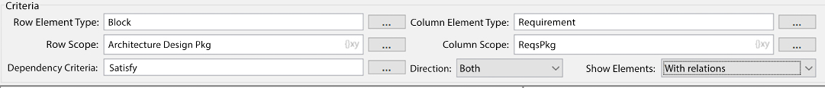
Figure 5.38: Satisfy matrix view layout

Add trace links

There are a couple of ways to populate the «satisfy» relations from the blocks. In this case, I prefer to diagram the relations rather than work in the matrix directly. The reason is that on the diagram, I can see the text of the requirement, while in the matrix, I can only see the name of the requirement.

Figure 5.39 shows one of the requirement diagrams created to create the relations:

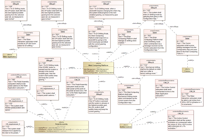
Figure 5.39: Example requirements diagram to add satisfy relations

Review traces

Figure 5.40 shows a portion of the resulting allocation relations from the subsystem elements to the requirements. The property with relations is used to only show rows and columns where a relation exists:

Figure 5.40: Subsystem-Requirement satisfy matrix

It is common to also show a matrix view where no relations exist. This allows easy identification of requirements not allocated to design elements or design elements that have no relation to the requirements. See Figure 5.41:

Figure 5.41: Subsystem-Requirements satisfy matrix – missing relations

Effective Reviews and walkthroughs

At the beginning of this chapter, I talked about reviews being the easiest but weakest form of model verification. This shouldn’t be construed to mean that I don’t believe reviews have value. Properly applied, reviews are a very useful adjunct to other, more rigorous forms of verification. Reviews can contribute to both syntactic (“compliance in form”) and syntactic (“compliance in meaning”) verification. They are relatively easy to perform and can provide input that is otherwise difficult to obtain.

Syntactic reviews, performed by quality assurance personnel, demonstrate compliance of the model to the project modeling guidelines, including the organization of the model, the presence of required elements and views, the structuring of those views, compliance with naming conventions, and more.

Semantic reviews are performed by Subject Matter Experts (SMEs). Some of the questions such reviews can address include:

• Does the model appropriately cover the necessary subjects (breadth)?
• Does the model include an appropriate level of detail (depth)?
• Is the level of precision, accuracy, and fidelity appropriate?
• Does the model accurately represent the physics of the situation?
• Are relevant standards properly taken into account?
• Is the technology accurately represented?
• Are all primary (“sunny day”) conditions considered?
• Are exceptional and edge cases (“rainy day”) cases adequately addressed?
• Is there anything of significance missed or inappropriately modeled?
• How will the correctness be verified?
• Is the information (typically the views) consumable by the stakeholders?

Reviews can be a valuable adjunct to other verification means. However, it is easy, and far too common, to perform them poorly in ways that are both expensive and ineffective. Reviews are very expensive because they typically have several people engaged for a significant number of hours. It is imperative that the meeting time is used efficiently. It is common for people to come unprepared, wasting others’ time with questions to which they should already have answers. It is also common to “go down the rabbit hole” in exploring solutions – that is, out of scope of the review. It is enough to identify the problem and move on. If a reviewer has a suggestion for a solution, they can present it to the author after the meeting. Further, because authors are putting their egos on the line, it is important that review comments address the product aspects and not what the author did wrong (“The product has this defect”, not “You made a mistake here”). Subsequent reviews of the same product should be limited solely to the resolution of action items, unless new information appears that invalidates the previous review.

The recipe described here is adapted from the notion of Fagan inspections, which were originally a means for software source code review (https://en.wikipedia.org/wiki/Fagan_inspection). I’ve adapted them to apply to engineering work products in general and especially to models.

Purpose

All models are abstractions but some are useful abstractions. A review ascertains whether they are the right abstractions covering the appropriate topics with adequate precision, depth, and breadth and represent the system correctly in such a way that the model fulfills its intended purpose.

The recipe provided here is very general and can be applied to any technical work product, but our focus will be on the review of models and their content and views.

Note that this recipe describes how to conduct a review only. There are other reasons to have meetings with technical work products, including the dissemination of information held within the work product. Those may be valid and important meetings to have but they are not reviews.

The purpose of a review is to verify the content of a collection of project data, either syntactically, semantically, or both.

Inputs and preconditions

A body of work is completed to the extent that the project can profitably conduct a review.

Outputs and postconditions

The primary outcomes are either a quality assurance record that the review was performed and no significant defects or issues were found, an action list of issues for the product authors to resolve, or both.

How to do it

Figure 5.42 shows the workflow for the recipe. A couple of main points in the figure should be emphasized.

First, the reviewers are expected to come to the review having examined the work products in detail. This is not a meeting for explanation, although questions of clarification are permitted. Second, solutions to identified issues are not discussed; suggestions can be discussed directly with the author after the review. Lastly, subsequent reviews are limited to the resolution of the action items from previous reviews:

Figure 5.42: Conduct review workflow

Establish the purpose of the view

Real models are too large to be reviewed in their entirety in a single review. Each review must have a specific purpose or intent that can be performed in a reasonable timeframe and consider only the subset of the model relevant to that purpose. Some common review intents are performing the following actions:

• Evaluate and understand systems engineering handoff models.
• Evaluate the use cases and their details.
• Evaluate architectural models.
• Evaluate design models.
• Evaluate the adequacy and coverage of a test plan and its details.
• Evaluate the result of the actions taken after a previous review.

Prepare materials for review

In this step, the material is gathered together for review. There are almost always multiple artifacts that are reviewed together. For example, a review of a use case model usually includes the following artifacts:

• Relevant use case diagrams
• Corresponding requirement text
• Use case sequence diagrams
• Use case state machines and activity diagrams
• Quality of service constraints
• Use case descriptions
• List of actions from previous reviews (if applicable)

For the review of a design model, common artifacts include:

• For each use case in the design model:
  • Block definition diagram(s) showing the collaboration of elements realizing the use case
  • Internal block diagram(s) showing how the collaborating elements connect
  • Original use case sequence diagram(s)
  • Elaborated design sequence diagrams showing the interaction
  • State machine diagrams for stateful classes
  • Activity diagrams for complex algorithms
  • List of actions from previous reviews (if applicable)

In Cameo, smart packages are special packages that contain elements by reference. An element can be added manually (such as by drag and drop) or automatically by defining criteria for inclusion. This feature can be used to gather up the packages, model elements, and diagrams relevant to a particular review.

Assign reviewer roles

Reviews have a number of roles that people can fulfill during the review. These need to be assigned to actual people to play those roles:

• Review coordinator:

This role organizes and runs the meeting, ensuring compliance with the review’s rules of conduct, such as “Direct comments to product, not the author” and “Discuss solutions with the author after the meeting.”

• Product owner/presenter:

This is generally one of the authors of the material under review. This person is technically knowledgeable and can answer questions of clarification during the meeting.

• SME reviewer:

This role is expected to provide a critical eye from a semantic viewpoint, whether it is about the specific technology, tool use, or engineering.

• Quality Assurance (QA) reviewer:

The QA role is there to ensure syntactic correctness and review the work product for compliance with relevant standards, including both internal standards (such as modeling guidelines and process definition) and external standards (such as industry or regulatory standards).

• Scribe:

The scribe takes the meeting minutes and creates and updates the action list, the list of actions and issues to be addressed after the meeting. The action list will serve as the basis for subsequent reviews of the work product.

Disseminate materials for review

The materials should be in the hands of the reviewers no less than 2 nor more than 14 days prior to the review.

Schedule review

The room for the review – along with any special equipment required (e.g., projector, whiteboards, internet connection, computer, modeling tool availability, etc.) – is scheduled and invitations issued to the reviewers. This may also be done virtually.

Reviewers independently inspect materials

The time to read the materials is not within the review meeting itself! The reviewers should come to the meeting with comments and issues they want to address. For complex work products, there may be value in the authors presenting a tutorial of the information to be reviewed. However, this should be a separate meeting, done prior to the review.

If the work product being reviewed is a model, then either the reviewers must have access to the relevant modeling tool, a web-based review environment (such as Cameo Collaborator), or reports must be generated for the purpose of the review that show the model content in an accessible format, such as Word, PowerPoint, or PDF.

Collectively discuss reviewer comments

Each issue or comment from a review should be heard and addressed by the product owner. If it is determined to be an issue, the issue is specified on the list of actions to be resolved.

DO NOT discuss solutions during this meeting. If someone has a solution they want to offer, have them do it outside the meeting with the work product owner.

Capture issues as action items

The primary outcome of the review is either an approval OR a set of action items to be resolved. Some action items might require modification to the work product, while others might require exploration or a trade study.

The action item list must be captured and will be used as the agenda for any subsequent reviews of the same work product set.

Resolve action items

As a result of the list of actions identified in the review, the product owner must modify the model or in some way address each of the issues. Then, if the changes are not trivial, a follow-up meeting is planned (repeat the recipe from the first step).

Plan review of action item resolutions

Unless the action items are considered trivial and not worth following up, a subsequent meeting should be scheduled specifically to address what was done to resolve the action items, and, typically, nothing more.

This subsequent review is performed in the same fashion as the original review.

Example

Let’s consider doing a review of one of the use cases from the Pegasus system, Emulate Front and Rear Gearing, presented as an example in the Functional analysis with state machines recipe.

Establish the purpose of the view

The primary outcomes of use case analysis are:

• Ensure a good set of requirements.
• Define system interfaces necessary to support the related requirements.

The purpose of the review is to examine the work products created to perform that analysis and its outputs to ensure that the analysis was done adequately for the need and that the work products fulfill their purpose.

Prepare materials for review

The purpose of the review will be to look at the work products around:

• The use case and associated actors and their key properties (such as description):
  • Use case diagram showing actors and related use cases.
  • Traced requirements – use case diagram showing traced requirements.
• The use case sequence diagrams:
  • Specification scenarios.
  • Animated scenarios.
• The use case execution context:
  • BDD/IBD showing the use case block and actor blocks.
• Use case block specification:
  • State and/or activity diagram for a use case or use case block.
  • State and/or activity diagrams for the actors or actor blocks.
  • Value and flow properties owned.
• Data schema:
  • BDD showing information known or relevant to the use case, including value types, dimensions (quantity kind), and units.
• The interfaces needed to support the use case:
  • BDD showing the interface blocks and their supported flow properties, operations, and event receptions.

Collectively, these diagrams and views form the work product to be reviewed. They are shown in Figure 2.32 through Figure 2.42 in Chapter 2, System Specification.

Assign reviewer roles

This step identifies the various roles. The review coordinator and the scribe are singletons – there is only one of those in the review. There must be at least one product owner (author) to present the materials and answer questions. The QA reviewer is optional but, if present, is usually a single person. There may be multiple SME reviewers, however. For the purpose of this example, let’s assume 2 software, 1 mechanical, 2 electronic, 1 system engineer, and 1 marketer are invited as SMEs.

The identified personnel must be notified of their responsibilities.

Disseminate materials to reviews

In this case, some of the SMEs may not have access to the modeling tool and may not be skilled in SysML (I’m looking at you, marketing). For those reviewers, we can print out a report of the parts of the model relevant to their concern, such as a requirements table for the marketing SME. Other SMEs who have access and skill with the modeling tool can either be granted access to the model in a shared repository or even emailed the model.

Schedule review

Scheduling the meeting is generally easy but finding a time available for all attendees can be a challenge.

Reviewers independently inspect materials

This is a place where compliance can be spotty, especially when the workflow is introduced. In my experience, it is common for people who “meant to get around to” reviewing the materials to show up unprepared and expect to be walked through the materials they were expected to already examine. It is better to cancel a review if most people haven’t reviewed the materials and reschedule than to waste everyone’s time.

Here, the reviewers are expected to examine the use case, requirements, structural and behavioral views for syntactic conformance (in the case of the QA reviewer) and semantic correctness (in the case of the engineering SMEs). The marketer here is serving as a proxy for the customer (training athlete) and should look for the appropriateness and quality of the requirements.

Sidebar: Recording review comments in the model in Cameo.

There are many ways to make and record comments. Here is a method I like to use when reviewing Cameo models.

In the model, I create a _Reviews package to hold the review comments. In this package, I create nested packages, one per reviewer or review. In these nested packages, I add Problem elements identifying the issues found. Since Problem is a kind of Comment, I can anchor the problem to the element manifesting the concern, whether it is a diagram, block, operation, value property, state, action, etc. Then in the specific review package, I create a table summarizing my comments along with the annotated elements. This latter column can be added with the Columns tool for the generic table. Such a table is shown in Figure 5.43:

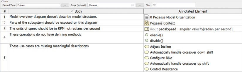
Figure 5.43: Review comment table

Collectively discuss reviewer comments

The comments often vary widely in terms of usefulness. Syntactic comments about spelling and standards conformance are useful, to be sure. Most useful are comments about semantic content. This will not only improve the product but also improve understanding and agreement among the attendees.

I believe in what is known as “ego-less” reviews, but they can seem a little awkward at first. The idea is that comments only refer to the work product and never to the author. You would never say, “You made a mistake here” to the author, but rather, “This requirement seems incorrect” or “There is a missing value property here.” This is an attempt to avoid hurt feelings and focus on the technical aspects of the work product.

Here are some (hypothetical) comments and issues that might be raised by the reviewers:

• QA reviewer: The use case diagram doesn’t have a mission statement, as defined by the modeling guidelines standard.
• QA reviewer: The requirements standard says that each use case should specify the reliability, in MTBF, of the service delivery. There is no requirement to specify reliability traced to the use case.
• Marketer: Requirement efarg17 says, “The default number of teeth for 12 cassette rings shall be 11, 13, 15, 17, 19, 21, 24, 28, 32, 36, 42, and 50. I think the gearing for the cassette should be from 12 to 28 instead.”
• Marketer: Requirement efarg19 says that “the default starting gear should be the smallest possible gear.” I think that’s ok for the very first ride, but subsequent rides should start up in the last gear the rider used.
• SME 1: The use case block has a value property cassette of type int. It isn’t clear whether the value being held is the number of teeth of the currently selected cassette or which cassette is in use. Please either add a comment or rename the value property to make that clear.
• SME 2: The name of the state ChangeGearing for the use case block state machine is misleading. It is actually waiting for a gear change, not performing a gear change while in that state.

The product owner can respond to these comments, and a discussion of the comment ensures. Some action items may be resolved as not requiring action because of a corrected misunderstanding on the part of the reviewer or as inconsequential. The group may decide that other issues must be acted upon, and these end up as action items.

Capture issues as action items

The scribe records the action items and may add annotations depending on the urgency or criticality of the concerns. After the meetings, the action items are typically sent to all attendees so they can ensure their issues are properly recorded or understood.

Resolve action items

The product owner can then address the concerns. In this case, they can add the missing mission statement to the use case diagram, add reliability requirements, change the name of the value property to cassetteIndex, and the name of the state of WaitingToChangeGear.

Plan review of action item resolutions

Since the changes are minor, the group can decide that a subsequent review isn’t needed.

Managing Model Work Items

There are many ways to manage to do items or work items in a backlog. This recipe is one specific way to simply and easily manage work items within a model. I’ve found this an effective way to track and enact changes in models on projects.

Purpose

The purpose of this recipe is to allow model authors to track, manage, and enact work items for a model.

Inputs and preconditions

The input for this recipe is an existing model that has work to be performed on its elements.

Outputs and postconditions

The primary output is an updated model that contains not only the changes made but also a record of changes, along with their priority and status.

How to do it

Figure 5.44 shows the workflow for this recipe.

There are two flows within the recipe. The first adds new work items and assigns their properties, while the second resolves the work items:

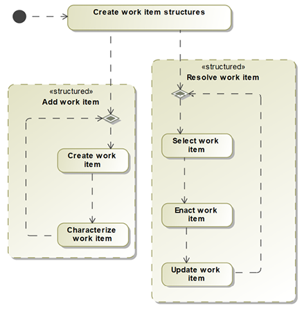
Figure 5.44: Manage work items

Create work item structures

This action adds the structures to represent, organize, and visualize the work items. We must define a work item as a type of element we can create and add relevant properties to it. The most obvious properties of such a type would be its status and its priority. The status of the work item identifies whether or not it is accepted or rejected, and whether it is waiting to be worked on, currently being worked on, or resolved. Additionally, a diagram or table should be defined so that we can easily see the work to be done.

Create work item

Once the work item types, structures, and visualization are defined, they can be used to characterize work items; as they are identified, they can be added to the list

Characterize work item

In this step, the properties of the work item are clarified. These properties are likely to include at least the work to be done, the status of the work item, and its priority.

Select work item

The other side to this recipe is performing the work. The first step is to select the work item to be resolved. Ideally, the work items are resolved on a higher-priority first basis.

Enact work item

This step is “simply” modifying the model to resolve the work item.

Update work item

Once the work has been performed, the status of the work item should be updated. Additionally, you may want to record how the work item was resolved.

Example

Create work item structures

In this example, we define a Work Item Profile that creates Work Item (a stereotype of Comment) and defines metadata properties status, priority, and resolution. The first two tags are typed by enumerations and the last is typed by String. It is possible to add other metadata, such as the type of work item (such as user story or spike), the author of the work item (for example, a particular quality assurance reviewer or subject matter expert), the date of the work item creation, and the date of the work item resolution:

Figure 5.45: Work item profile

The reason for adding prefix numbers to the priority enumeration literals is so that you can sort the table of work items in a reasonable order, so that the TOP items appear before the URGENT items, which appear before the IMPORTANT work items, and so on.

Next, we must also define a place in our model to hold the work items and related elements. In this case, I create a package named Work Items to hold the work items to be added and to contain the visualization of those work items.

Finally, we must provide a visualization for the set of work items. Here, we will add a generic table of work items showing the target of the work items (if known) and the properties of the work item. Since Work Item is a stereotype of Comment – and we can anchor comments to model elements (including diagrams) – we can add Annotated Elements in the table as a column. Thus, as we add a work item, we can potentially anchor the work item to relevant model elements (if known), providing valuable guidance for its later resolution. Such a table, with a sample work item, is shown in Figure 5.46:

Figure 5.46: Work item table

Create work item

Now that the structures are in place, we can start adding work items. This might come from inspection and review (see the previous recipe Effective walkthroughs and reviews) or some other source such as user stories, spikes, defect reports, or technical work items from the project backlog.

Characterize work item

Because Work Item is a stereotype of Comment, you may add anchors to elements, although when the work item is created, the elements to be modified may not be obvious or known. The status should be initially set to PENDING and the priority of the work item should be specified. The easiest way to add an anchor is to place the work item on a relevant diagram and add the anchor. It is simple to create diagrams in the Work Items package and drag the relevant elements onto that diagram and add the anchors there. This is my preferred approach so the presence of the work items doesn’t “pollute” the other diagrams in the model. In Cameo, you can drag diagrams onto other diagrams, making it easy to add anchors to the model element to be modified in a diagram.

Figure 5.47 shows an example:

Figure 5.47: Adding anchors to model elements

The desired visualization for the work items is the work item table. Figure 5.48 shows an example, sorted in priority order:

Figure 5.48: Working work item table

Select work item

To resolve the work item, we must first select it.

Enact work item

This step involves updating the model to enact the required changes. The first step is to change the work item status to IN PROCESS.

Update work item

Once completed, the work item can be updated. At the very least, the status property is changed to RESOLVED. You might want to also update the priority to 8 – RESOLVED so that it isn’t mixed in with the work items yet to be resolved.

Test Driven Modeling

For the last recipe in the book, I’d like to present a recipe that is central to my view of the integration of modeling and agile methods. The archetypal workflow in software agile methods is test-driven development (TDD), in which you do the following:

    Loop
        Write a test case
        Write a bit of code to meet that test case
        Apply test case
        If (defect) fix defect
    Until done

It’s an appealing story, to be sure. Each loop shouldn’t take more than a few minutes. This is a key means in agile methods to develop high-quality code: test incrementally throughout the coding process.

TDD aligns with this Law of Douglass:

The best way not to have defects in your system is to not put any defects into your system.

Law of Douglass #30

See https://www.bruce-douglass.com/geekosphere for further information.

This points out that it is far easier to develop high-quality systems if you avoid entering defects rather than putting defects in and trying to identify, isolate, and correct them sometime in the future. TDD is a way to do that.

The same kind of approach is possible with respect to developing models, particularly executable models, an approach I call Test-Driven Modeling (TDM). These models needn’t be limited to design models; they can also be models of architecture, requirements, or any kind of computational model. Such models can be developed in small, incremental steps and verified as the model evolves.

When it comes to modeling, this is not what people typically do. Most people build huge monolithic models before deciding to verify them. I remember one consulting customer who had a state machine with 800+ states. They had put it together and then attempted to “beat it with the testing stick” until it worked. They gave up after several months without ever getting it to even compile, let alone run properly. Then they called me.

The first thing I did was discard the expensive-yet-unworkable state machine and developed an equivalent using this TDM recipe. Each small iteration, known as a nanocycle in the Harmony aMBSE process (see Agile Systems Engineering by Bruce Douglass (Morgan Kaufmann, 2016) for further information) is executed anywhere from 30 to 60 minutes. In less than a week, the completed state machine was compiling, running, and working. It was then possible to uncover a number of subtle, yet important, specification defects from their source material.

Like I said, TDM is not the way most people create models. Let’s change that.

Purpose

The purpose of this recipe is to quickly develop a demonstrably correct model by frequently executing and running the model.

Inputs and preconditions

The input is a well-defined modeling objective that can be rendered with executable modeling constructs.

Outputs and postconditions

The output is a well-constructed, executable, and verified model.

How to do it

Figure 5.49 shows the basic flow. I would take care to note that I don’t really care whether the test case is created just prior to the “Model a bit” step or just after; it is essentially at the same time. Classic TDD has the test case definition first, but it doesn’t really matter to me.

The primary point is that the test case isn’t defined weeks to months after the design work is done but is done continuously as the work product is developed:

Figure 5.49: TDM

Define the test case

This step can come immediately before or after the Model a bit step, but logically they are done at about the same time. The test case defines a Minimal Testable Feature (MTF), sometimes known as a Minimal Verifiable Feature (MVF), that is to be modeled in this particular nanocycle. The MTF in this context is a small evolution of the model from its current state, enroute to the complete model that satisfies the initial modeling objective. The tendency is to make the nanocycles too large, so keep them short. The properties of the MTF to strive for are:

• The feature can be modeled in a few (<30) minutes.
• The feature tests differently from the previous model’s condition.
• The feature contributes to the modeling objective that the sequence of nanocycles is intended to achieve.

For example, suppose the modeling objective is to construct an executable use case. Each nanocycle would add one or more requirements to the use case model, such that the state machine adds a few transitions, actions, or states. A state machine with 30 states and 40 transitions might be done as a series of 10–15 nanocycle iterations, each of which has a small MTF evolution.

Model a bit

In this step, the model is evolved by adding a small number of features: a value property or two, perhaps a couple of transitions, a state, or a small set of other model elements.

Apply the test case

At this point, you have a (small) model evolution and a (small) test case. In this step, you apply the test case to ensure that it is modeled correctly.

Fix defects

If the model fails the test, it is fixed in this step.

The nanocycles repeat until the initial modeling objective is satisfied.

Example

I want to introduce my favorite example for TDM. I’ve used this example in numerous courses and found it to be instructive and accessible to my students. I’ve even done the experiment: I told some groups to develop the model without giving them guidance (and they all tried to do it in a single step) or gave them an explicit instruction to do it in several separate steps, with a short description of the MTF increments. The results are that, in the time frame allotted, 100% of the unguided groups failed while 80% of the nanocycle groups succeeded.

The problem

Consider an intersection Traffic Light Controller (TLC). The TLC controls traffic (via lights) on a primary road and a secondary road. The roads contain both through-lane traffic and left-turn lane traffic. In addition, the TLC also controls pedestrian traffic along those roads as well (again, via lights). The basic control rules are:

• In the absence of both pedestrians and left-turn cars, the through lights operate entirely based on time:
  • Turn lane lights remain red; pedestrian lights remain DON’T WALK.
  • All lights are red for RED TIME.
  • The through lanes (both direction for a given road) go green for GREEN TIME, while cross traffic lights are red while cross traffic remains stopped.
  • The through lanes (again, in both directions) go yellow for YELLOW TIME.
  • The through lanes all turn red and the cross traffic gets to go next, using the same flow.
  • Repeat forever.
• If cars are present in the left turn lane for a given road, the behavior is slightly different:
  • When a road is ready to set through traffic green but there is a car waiting in that road’s left turn lane, the turn lanes (both directions on the same road) go first, and the through lane remains red:
    • Turn lanes go green for GREEN TIME
    • Turn lanes go yellow for YELLOW TIME
    • Turn lanes go red for RED TIME
    • Now the through lanes can continue normally
• If pedestrians are waiting to cross a road (that is, they want to cross the cross-traffic road), then the behavior is modified:
  • When the through light goes green, the pedestrian light displays “Walk” for WALK TIME.
  • The pedestrian light then displays flashing “Don’t Walk” for RUN TIME.
  • The pedestrian light then displays a solid “Don’t Walk” and the through light now goes yellow for YELLOW TIME.
  • The through lane proceeds normally.

I like this example because it is easy to describe, it is conceptually simple, and it is very familiar.

Since this is a short, iterative cycle, we’ll just run the cycle multiple times in the example:

• MTF 0: Single through traffic light
• MTF 1: Primary and secondary through lights
• MTF 2: Add turns lights
• MTF 3: Add pedestrians

Define test case: MTF 0: Episode III: The Revenge of the Through Light

Let’s define the first MTF step.

Test case: Single light should go through the colors in the right sequence with the right timing – red for RED TIME, green for GREEN TIME, and yellow for YELLOW TIME.

Model a bit: MTF 0: Episode III: The Revenge of the Through Light

Evolution: Add a single traffic light that cycles through its colors.

This model is pretty simple. It consists of two blocks: Traffic Light Control System (which will also serve as our tester) and Traffic Lane, with a single, directed composition from the former to the latter. We need to define the timings – I used value properties in the Traffic Lane block with the readOnly property set. I also added an enumerated type COLOR_TYPE to define the different colors.

A setcolor(color: COLOR_TYPE) just prints out the value of the color to standard output for the purpose of this model. This simple model is shown in Figure 5.50:

Figure 5.50: Structure and behavior for MTF 0

Apply test case: MTF 0: Episode III: The Revenge of the Through Light

Now let’s run the model. In Cameo, right-click the Traffic Light Control System block and select Simulation > Run. When we run, we manually insert the exStart event to the Traffic Light Control System to kick it off, and we can view the execution outcomes in Figure 5.51:

Figure 5.51: Running MTF 0

We’ve now completed our first nanocycle. It was very short – and it didn’t do much – but we quickly got it to work.

Define test case: MTF 1: Episode IV: A New Hope (For the Secondary Through Lane)

Let’s define the next MTF step.

Test case: Both roads should cycle through the lights, with cross traffic held red while the current lane cycles through.

Model a bit: MTF 1: Episode IV: A New Hope (For the Secondary Through Lane)

Evolution: Add a second composition to the through lane to add the secondary road; the system now contains two traffic light instances. Modify the state machine of the traffic light so that the two instances of Traffic Lane can properly coordinate. In this case, we add proxy ports pOutThru and pInThru, both typed by the interface block ibLane. One of these ports is conjugated so that it can send and receive the same event, though via different ports. See Figure 5.52:

Figure 5.52: Structure for MTF 1

In the figure, we take advantage of Cameo’s ability to show diagrams on other diagrams to show the internal block diagram contents on the block definition diagram.

The state machine for the Traffic Light Control System is exactly the same except that it now sends the evGo event to both instances and the signal has an additional attribute. The first (Boolean) value tells the instance whether it should go first or wait. The second gives the instance its identity for the whoAmI value property. Figure 5.53 shows the state machine for Traffic Light Control System along with the behaviors to send the evGo signal to initialize the two traffic lights. Figure 5.54 shows the Traffic Lane behavior:

Figure 5.53: Traffic Light Control System state machine for MTF 1

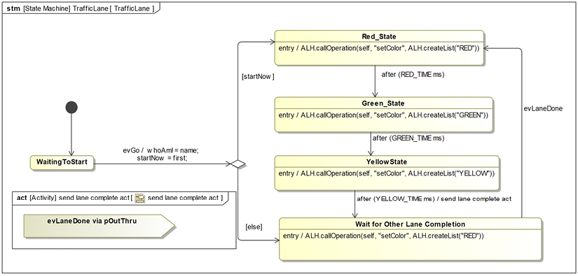
Figure 5.54: Traffic Lane state machine for MTF 1

Apply test case: MTF 1: Episode IV: A New Hope (For the Secondary Through Lane)

Now the model is getting interesting. Is it right? Let’s run the test case and see.

Figure 5.55 shows the outcomes, both in the animated sequence diagram and the output window.

The scenario is a bit small to read, but you can see in the output window that it operates as expected:

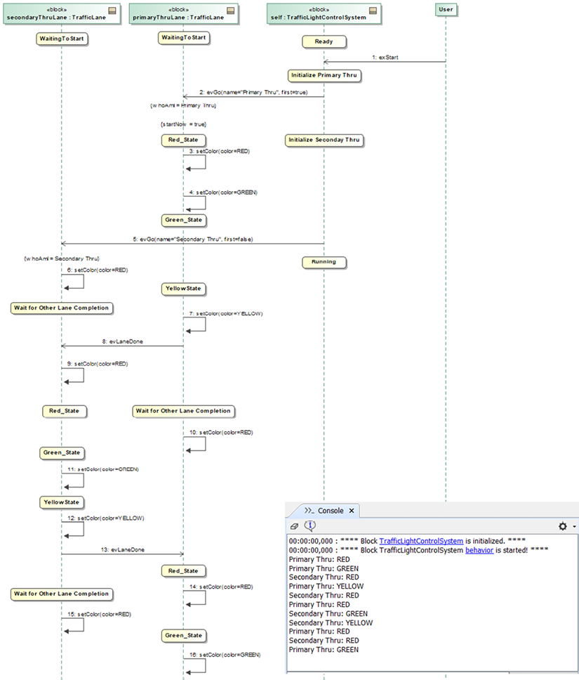
Figure 5.55: Running MTF 1

Fix Defects: MTF 1: Episode IV: A New Hope (For the Secondary Through Lane)

There are no defects to fix in this nanocycle.

Define test case: MTF 2: Episode V: The Turn Lane Strikes Back

Test case: When a car arrives on a road regardless of when in the cycle that occurs, the system properly allows turn lanes to cycle through, followed by the through light on the same road.

Test case: In subsequent cycles, the system “forgets” the turn lane was previously activated.

Model a bit: MTF 2: Episode V: The Turn Lane Strikes Back

Evolution: Add turn lanes and update state machines to manage them.

We must add two more lights to the system to support the left turn lanes, and make them composite parts of the Traffic Light Control System. In this case, the through lights and the turn lights are actually different types because while the through lights must coordinate with the cross-traffic through light, the turn lane coordinates in a different way with its corresponding road through light. We’ll make the Thru Lane and Turn Lane lights different subclasses of Traffic Lane, and remove the state behavior from the Traffic Lane base class. The structural model is shown in Figure 5.56:

Figure 5.56: Structure for MTF 2

The Traffic Light Control System internal block diagram (Figure 5.57) shows the expected connections among the instances:

Figure 5.57: MTF 2 IBD

The state machine for Traffic Light Control System is modified so that it starts the turn lane lights in addition to the through lane lights. See Figure 5.58:

Figure 5.58: State machine for traffic light system MTF 2

More interesting are the modifications to the Thru Lane and Turn Lane lights. The state machine in Figure 5.59 is for the Thru Lane and Figure 5.60 is for the Turn Lane. The send actions on the state machines show the coordination of the through lanes as well as between the through lane and its connected turn lane:

Figure 5.59: MTF 2 through lane states

Figure 5.60: MTF 2 turn lane states

Apply test case: MTF 2: Episode V: The Turn Lane Strikes Back

Running the test case results in long sequence diagrams, so we will simply look at the output console window to verify the correctness of the execution. In this case, we’ll start the system and while the primary through lane is green, we will have a car arrive for the secondary turn lane. The expected behavior is that the primary light will go green, yellow, and then red. Then, because there is a car waiting in the secondary turn lane, we expect to see the secondary turn lane go green, yellow, and then red. Following that, the secondary through lane should go green, yellow, and red before the primary through lane again goes green.

When running the state machine, we note that we cannot send the event exCarArrive at the right time because of a race condition. Because of the order in which the behavior unfolds, the primary through lane – being initialized first – starts cycling through its behavior even while the Traffic Light Control System is initializing the other parts. This is a classic race condition.

To fix this problem, we will change the behavior of the state machines:

• evGo will no longer have a first parameter. Both through lanes will start in the Wait for Other Lane Completion state.
• At the end of initialization, the Traffic Light Control System will send the evLaneDone signal to the Primary Thru Lane part to kick things off.

The updated behavior for the Traffic Light Control System is shown in Figure 5.61:

Figure 5.61: Traffic light control system updated behavior

The change to the Thru Lane is simpler. See Figure 5.62:

Figure 5.62: Updated thru lane behavior

Now we can run the model and while the Traffic Light Control System waits for the exStart event, we can send the exCarArrive signal to the secondary turn lane part to simulate the arrival of a car in that lane.

In Cameo, when the context has multiple parts of the same type, it isn’t obvious how to send the signal to the correct part. The trick is to look in the Variables section of the Simulation Toolkit and find the address of the part you want, match that address to a running behavior in the Sessions window, and then use the pull-down trigger list to send the event.

See Figure 5.63:

Figure 5.63: Sending the signal to the correct part

Figure 5.64 shows the console window output for the updated model:

Figure 5.64: Running MTF 2

Fix Defects: MTF 2: Episode V: The Turn Lane Strikes Back

The race condition has been identified and resolved.

Define test case: MTF 3: Episode VI: Return of the Pedestrian

Test case: When a pedestrian arrives on the secondary road and the primary through light is green, the pedestrian gets the walk light at the same time that the secondary through lane gets a green light.

Test case: When a pedestrian arrives on the primary road and the primary through light is currently green, the pedestrian gets a walk light the next time the primary through lane gets a green light.

Model a bit MTF 3: Episode VI: Return of the Pedestrian

Evolutions: Add pedestrians and update state behavior to manage them.

This last nanocycle adds the pedestrian crosswalks, and updates the behavior of the Traffic Light Control System and the through lanes to properly interact with them. The BDD shows the evolving structure (Figure 5.65) and the Traffic Light Control System IBD shows the connected design (Figure 5.66):

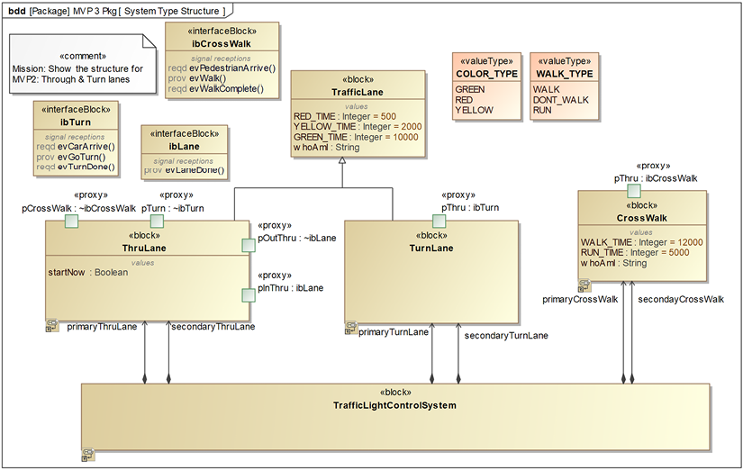
Figure 5.65: MTF 3 structure

Figure 5.66: Traffic light system IBD for MTF 3

The Traffic Light Control System has a minor change to its state machine to initialize and start the Cross Walk instances (Figure 5.67):

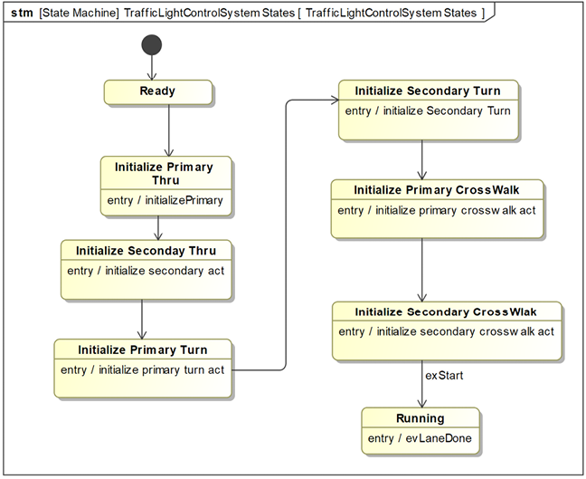
Figure 5.67: Traffic light system state machine for MV3

The state machine for the Thru Lanes adds an AND-state to keep track of whether pedestrians are waiting and a few states to handle the behavior when a pedestrian is crossing (Figure 5.68). If you compare this state machine with the Thru Lane state machine from MTF 2 (Figure 5.59), you can see that the updated state machine is a fairly simple evolution of its previous condition:

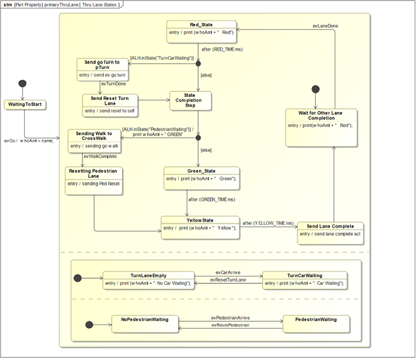
Figure 5.68: Thru lane state machine for MTF 3

Lastly, the state machine for the Cross Walk is straightforward, as can be seen in Figure 5.69.

Note that the Turn Lane state machine didn’t change from MTF 2:

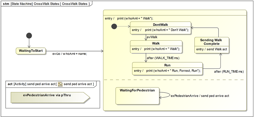
Figure 5.69: Cross walk state machine for MTF 3

Apply test case MTF 3: Episode VI: Return of the Pedestrian

The model is getting a bit complex to rely solely on the animated sequence diagrams for testing, so we elaborate the UI diagram by adding controls related to the pedestrian traffic and adding a simulation configuration to use as the user interface to monitor and control the simulation.

This MTF has two test cases; the output window in Figure 5.70 shows the outcome for test case 1:

Figure 5.70: Output from MTF 3 test case 1 run

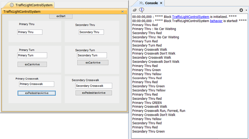
Figure 5.71: Output from MTF 3 test case 2 run

Fix defects MTF 3: Episode VI: Return of the Pedestrian

No defects were found. MTF 3 runs as expected.

This example illustrates that it was pretty simple to construct a (somewhat complex) model easily by developing it in small iterations and verifying its correctness so far before moving on.

Now that’s pod racing!... Er, TDM.

Join our community on Discord

Join our community’s Discord space for discussions with the author and other readers:

https://packt.link/cpVUC