
Chapter 12
Gaining NoSQL Access Using DynamoDB
IN THIS CHAPTER
![]() Defining the DynamoDB service feature set
Defining the DynamoDB service feature set
![]() Performing the DynamoDB setup
Performing the DynamoDB setup
![]() Creating the first practice database
Creating the first practice database
![]() Asking the practice database questions
Asking the practice database questions
The Structured Query Language (SQL) associated with relational databases (those that use tables of related data) makes up the bulk of Database Management System (DBMS) applications today. Using Relational DBMS (RDBMS) strategies makes sense for most kinds of data because information such as accounting, customer records, inventory, and a vast array of other business information naturally lends itself to the tabular form, in which columns describe the individual data elements and rows contain the individual records.
 However, some data, such as that used by big data or real-time applications, is harder to model using an RDBMS. Consequently, NoSQL or non-SQL databases become more attractive because they use other means to model data that doesn’t naturally lend itself to tables. Because business, science, and other entities rely heavily on these nontraditional data sources today, NoSQL is more popular. DynamoDB is Amazon’s answer to the need for a NoSQL database for various kinds of data analysis. This chapter begins by helping you understand DynamoDB so that you can better use it to address your specific NoSQL needs.
Before you can do anything with DynamoDB, you need to set up and configure a copy on AWS. That’s where you’ll use it for the most part, after you get past the early experimentation stage, and it’s where the production version of any applications your organization develops will appear. The next section of this chapter looks at the process for using DynamoDB online.
The remainder of the chapter focuses on a test database that you create locally. You develop a simple database using a local copy of DynamoDB, perform some essential tasks with it, and then upload it to your online copy of DynamoDB. You usually follow this same path when working with DynamoDB in a real-world project.
Considering the DynamoDB Features
DynamoDB provides access to all the common NoSQL features, which means that you don’t need to worry about issues like creating a schema or maintaining tables. You use a NoSQL database in a free-form manner when compared to a SQL database, and NoSQL gives you the capability to work with large data with greater ease than a SQL database allows. The following sections provide you with a better idea of just what DynamoDB provides and why NoSQL databases are important to businesses.
Getting a quick overview of NoSQL
The main reason to use NoSQL is to address the needs of modern applications. At one time, developers created applications that resided on just one or two platforms. An application development team might work on an application upgrade for months and use a limited number of data types to perform data manipulation. Today, the application environment is completely different, making the use of RDBMS hard for modern applications. NoSQL addresses these needs in a number of ways:
- Developers no longer limit themselves to a set number of data types. Modern applications use data types that are structured, semistructured, unstructured, and polymorphic (a data type used with a single interface that can actually work with objects of different underlying types).
- Short development cycles make using an RDBMS hard, requiring a formal change process to update the schema and migrate the data to the new setup. A NoSQL database is flexible enough to allow ad hoc changes that are more in line with today’s development cycle.
- Many applications today appear as services, rather than being installed on a particular system. The use of a Service Oriented Architecture (SOA) means that the application must be available 24 hours a day and that a user can access the same application using any sort of device. NoSQL databases can scale to meet the demands of such an application because they don’t have all the underlying architecture of an RDBMS to weigh them down.
- The use of cloud computing means that data must appear in a form that works with multiple online services, even when the developers don’t know the needs of those services at the time that a development cycle begins. Because NoSQL doesn’t rely on formal schemas and access methodologies, it’s easier to create an environment where any service, anywhere, can access the data as needed.
- NoSQL supports the concept of auto-sharding, which lets you store data across multiple servers. When working with an RDBMS, the data normally appears on a single server to ensure that the DBMS can perform required maintenance tasks. The use of multiple servers makes NoSQL scale better and function more reliably as well, because you don’t have just one failure point. DynamoDB extends the concept of auto-sharding by making cross-region replication possible (see the article at
http://docs.aws.amazon.com/amazondynamodb/latest/developerguide/Streams.CrossRegionRepl.htmlfor more details). - Modern languages, such as R, provide data analysis features that rely on the flexible nature of unstructured data to perform its tasks. Because modern business makes decisions based on all sorts of analysis, it also needs modern languages that can perform the required analysis.
Most NoSQL databases provide several methods of organizing data. DynamoDB doesn’t support all the various types. What you get is a key-value pair setup, in which a key provides a unique reference to the data stored in the value. The key and the value are both data, but the key must provide unique data so that the database can locate a particular piece of information. A value can contain anything from a simple integer to a document to a complex description of a particular process. NoSQL doesn’t place any sort of limit on what the value can contain, which makes it an extremely agile method of storing data.
 NoSQL databases typically support a number of other organizational types that DynamoDB doesn’t currently support natively. For example, you can’t create a graph store that shows interactions of networks of data, such as those found in social media. Examples of NoSQL databases that do provide this support are Neo4J (
https://neo4j.com/) and Giraph (http://giraph.apache.org/). Fortunately, AWS recently added integration with Titan (http://titan.thinkaurelius.com/), a distributed graph database, to provide a level of this functionality.
DynamoDB also doesn’t support documents such as those found in MongoDB (https://www.mongodb.com/). A document is a complex structure that can contain key-value pairs, key-array pairs (an array can contain a series of like values), and even other documents. Documents are a superset of the key-value pairs that DynamoDB does support.
Finally, DynamoDB doesn’t support the specialized wide-column data stores found in products such as Cassandra (http://cassandra.apache.org/) and HBase (https://hbase.apache.org/). These kinds of data stores find use in large dataset analysis. Using this kind of data store enables databases, such as Cassandra and HBase, to group data in columns, rather than in rows, which is how most databases work.
Differentiating between NoSQL and relational databases
Previous sections of the chapter may lead you to believe that RDBMS development is archaic because it lacks support for modern agile development methods. However, RDBMS and NoSQL databases actually fulfill needs in two different niches, so a business often needs access to both kinds of data storage. Of course, that’s why AWS includes both (see Chapters 10 and 11 for more information about how AWS handles RDBMS requirements).
Even though NoSQL provides some significant advantages, you need to consider how an RDBMS can help your organization as well. The main consideration in favor of NoSQL is whether the data is unstable or especially complex. In this case, NoSQL presents the best strategy for storing the data because it provides the best flexibility options.
However, an RDBMS offers some special features as well. For example, an RDBMS offers consistency because of the schema that seems to hold it back in other areas. The schema ensures that the data in the database actually meets the criteria you set for it, which means that you’re less likely to receive incomplete, missing, errant, or otherwise unusable data from the data source. The consistency offered by an RDBMS is a huge advantage because it means that developers spend less time coding around potential data problems — they can focus on the actual data processing, presentation, and modification.
An RDBMS usually relies on normalization to keep the data size small. When working with a NoSQL database, you can see a lot of repeated data, which consumes more resources. Of course, computer resources are relatively inexpensive today, but given that you’re working in a cloud environment, the charges for inefficiencies can add up quickly. The thing to remember about having too much repeated data is that it also tends to slow down parsing, which means that a properly normalized RDBMS database can often find and manipulate data faster than its NoSQL counterpart can.
NoSQL and RDBMS databases offer different forms of reliability as well. Although a NoSQL database scales well and can provide superior speed by spreading itself over multiple servers, the RDBMS offers superior reliability of the intrinsic data. You can depend on the data in an RDBMS being of a certain type with specific characteristics. In addition, you get all the data or none of the data, rather than bits and pieces of the data, as is possible with a NoSQL database.
Because an RDBMS provides the data in a certain form, it can also provide more in the way of built-in query and analysis capabilities. Some of the major RDBMSs provide a substantial array of query and analysis capabilities so that developers don’t spend a lot of time reinventing the wheel, and so that administrators can actually figure out what data is available without also getting a degree in development. When the form of the data is right (the lack of a wealth of large objects), an RDBMS can also present results faster because the organization makes parsing the information easier. DynamoDB partially offsets the enhanced query capabilities of an RDBMS by providing a secondary index capability (read more at http://docs.aws.amazon.com/amazondynamodb/latest/developerguide/SecondaryIndexes.html).
As with many data issues, no one single database solution works well in every case. Both RDBMS and NoSQL databases have definite places in an organization. In fact, that’s why some vendors offer both solutions and some are working on methods to integrate the two. Interoperability between RDBMS and NoSQL databases is becoming more common with the development of APIs for products such as MongoDB by IBM (see the series of articles that begins at http://www.ibm.com/developerworks/data/library/techarticle/dm-1306nosqlforjson1/ for details). IBM is creating a data representation, query language, and wire protocol to make DB2 and MongoDB interactions relatively seamless.
Defining typical uses for DynamoDB
Most of the use cases for DynamoDB found at https://aws.amazon.com/dynamodb/ revolve around unstructured, changeable data. One of the more interesting uses of DynamoDB is to provide language support for Duolingo (https://www.duolingo.com/nojs/splash), a product that helps people learn another language by using a gamelike paradigm. Making learning fun generally makes it easier as well, and learning another language can be a complex task that requires as much fun as one can give it.
Obtaining a continuous stream of data is important in some cases, especially in monitoring roles. For example, BMW uses DynamoDB to collect sensor data from its cars. The use of streams in DynamoDB (see http://docs.aws.amazon.com/amazondynamodb/latest/developerguide/Streams.html for more information) makes this kind of application practical. Dropcam (https://nest.com/camera/meet-nest-cam/), a company that offers property monitoring, is another example of using streaming to provide real-time updates for an application.
DynamoDB actually provides a wide range of impressive features, which you can read about at https://aws.amazon.com/dynamodb/details/. The problem is finding use cases for these new features, such as ElasticMap Reduce integration, in real-world applications today. The lack of use cases is hardly surprising because most of this technology is so incredibly new. The important takeaway here is that DynamoDB has a place alongside RDS for more organizations, and you need to find the mix that works best for your needs.
Creating a Basic DynamoDB Setup
You have a number of ways to work with DynamoDB, many of which apply more to DevOps, DBAs, or developers than they do to administrators. For example, you can go with the local option described in the upcoming “Working with DynamoDB locally” sidebar. This option appeals mostly to developers because it lets a developer play with DynamoDB in a manner that combines it with languages that work well with NoSQL databases, such as Python. If you’re truly interested in development as well as administrative tasks, you can find some helpful details in the sidebar.
Before you can do anything with DynamoDB, you must create an instance of it, just as you do for RDS. The following procedure helps you get started with DynamoDB so that you can perform some interesting tasks with it:
- Sign into AWS using your administrator account.
-
Navigate to the DynamoDB Management Console at
https://console.aws.amazon.com/dynamodb.You see a Welcome page that contains interesting information about DynamoDB and what it can do for you. However, you don’t see the actual console at this point. Notice the Getting Started Guide link, which you can use to obtain access to tutorials and introductory videos.
-
Click Create Table.
You see the Create DynamoDB Table page, shown in Figure 12-1. Amazon assumes that most people have worked with an RDBMS database, so the instructions for working with RDS are fewer and less detailed. Notice the level of detail provided for DynamoDB. The wizard explains each part of the table creation process carefully to reduce the likelihood that you will make mistakes.
-
Type TestDB in the Table Name field.
Pick a descriptive name for your table. In this case, you need to remember that your entire database could consist of a single, large table.
-
Type EmployeeID in the Primary Key field and choose Number for its type.
When working with a NoSQL database, you must define a unique value as the key in the key-value pair. An employee ID is likely to provide a unique value across all employees. Duplicated keys will cause problems because you can’t uniquely identify a particular piece of data after the key is duplicated.
A key must also provide a simple value. When working with DynamoDB, you have a choice of making the key a number, string, or binary value. You can’t use a Boolean value because you would have only a choice between true and false. Likewise, other data types won’t work because they are either too complex or don’t offer enough choices.
 Notice the Add Sort Key check box. Selecting this option lets you add a secondary method of locating data. Using a sort key lets you locate data using more than just the primary key. For example, in addition to the employee ID, you might also want to add a sort key based on employee name. People know names; they tend not to know IDs. However, a name isn’t necessarily unique: Two people can have the same name, so using a name as your primary key is a bad idea.
Not shown in Figure 12-1 is the option to Use Default Settings. The default settings create a NoSQL table that lacks a secondary index, allows a specific provisioned capacity, and sets alarms for occasions when applications exceed the provisioned capacity. A provisioned capacity essentially determines the number of reads and writes that you expect per second. Given that this is a test setup, a setting of 5 reads and 5 writes should work well. You can read more about provisioned capacity at
http://docs.aws.amazon.com/amazondynamodb/latest/developerguide/HowItWorks.ProvisionedThroughput.html. -
Select Add Sort Key.
You see another field added for entering a sort field, as shown in Figure 12-2. Notice that this second field is connected to the first, so the two fields are essentially used together.
- Type EmployeeName in the sort key field and set its type to String.
-
Click Create.
You see the Tables page of the DynamoDB Management Console, shown in Figure 12-3. This figure shows the list of tables in the left pane and the details for the selected table in the right pane. Each of the tabs tells you something about the table. The More link on the right of the list of tabs tells you that more tabs are available for you to access.
Not shown in Figure 12-2 is the Navigation pane. Click the right-pointing arrow to show the Navigation pane, where you can choose other DynamoDB views (Dashboard and Reserved Capacity).

FIGURE 12-1: Start defining the characteristics of the table you want to create.

FIGURE 12-2: Choose a sort key that people will understand well.

FIGURE 12-3: The table you created appears in the Tables page.
Developing a Basic Database
The act of creating a table doesn’t necessarily mean that your database is ready for use. For one thing, even though you have the beginnings of a database, it lacks data. Also, you may need to modify some of the settings to make the database suit your needs better. For example, you may decide to include additional alarms based on metrics that you see, or to increase the capacity as the test phase progresses and more people work with the data.
Normally, you populate a database by importing data into it. The DynamoDB interface also allows you to enter data manually, which works quite well for test purposes. After the data looks the way you want it to look, you can export the data to see how the data you want to import should look. Exporting the data also allows you to move it to other locations or perform a backup outside of AWS.
Databases normally contain more than one table, even NoSQL databases. Yes, creating a simple test database using a single table is possible, but multiple tables appear more often than not in a database. The examples in this chapter do rely on a single table — the one you create in the previous section. You use this table in the sections that follow to explore the techniques that DynamoDB provides for interacting with tables and the data they contain.
Configuring tables
The right pane in Figure 12-3 contains a series of tabs. Each of these tabs gives you with useful information about the selected table. Because the information is table specific, you can’t perform actions on groups of tables using the interface. The following sections discuss the essentials of working with tables.
Working with streams
Because of the manner in which NoSQL tables work, you often need to synchronize copies of the same data. A table in one region might receive changes that you also need to replicate in another region. In fact, you might find other reasons to provide a log of changes (think of the log as a detailed procedure you could use to replicate the changes) to the tables you create. A stream is a record of table changes (the actual data used to modify the table, rather than a procedure detailing the tasks performed, as provided by a log). Each change appears only once in the log you create, and it appears in the order in which DynamoDB received the change. The ordered list enables anyone reading the log to reconstruct table changes in another location. AWS retains this log for 24 hours, so it doesn’t need to be read immediately.
The Overview tab contains Manage Stream button you click to set up a stream for your table, as shown in Figure 12-4. This feature isn’t enabled by default, but you can configure it to allow the storage of specific change information. You have the following options when creating the change log:
- Keys Only: Just the key portion of the key-value pair appears in the log. This option has the advantage of providing just a summary of the changes and makes the log smaller and easier to read. If the receiving party wants to do something with the change, the new value can be read from the table.
- New Image: Both the new key and value of the key-value pair appear in the log. The log contains the information as it appears after the modification. This is the right option to use for replication, in that you want to copy both the new key and value to another table.
- Old Image: Both the old key and the value of the key-value pair appear in the log. This log entry shows how the table entry appeared before someone modified it.
- New and Old Images: The entire new and old key-value pairs appear in the log. You can use this kind of entry for verification purposes. However, realize that this approach uses the most space. The log will be much larger than the actual table because you’re storing two entries for absolutely every change made to the table.

FIGURE 12-4: Use the Stream option to create a log of table changes.
Viewing metrics
The Metrics tab contains a series of graphs, which you can expand by clicking the graphs. Metrics help you understand how well your table is working and enable you to change settings before a particular issue becomes critical. Many of the metrics tables include multiple entries. For example, in the Read Capacity metric, shown in Figure 12-5, the red line shows the provisioned read capacity and the blue line shows how much of that capacity your application consumes. When the blue line starts to approach the red line, you need to consider modifying the read capacity of the table to avoid throttled read requests, which appear in the metric to the right of the Read Capacity metric.

FIGURE 12-5: Metrics help you manage your table.
The i shown in the circle next to a metric graph tells you that you can get additional information about that graph. Hover your mouse over the i to see a pop-up containing helpful information. For example, the pop-up for the Read Capacity graph tells you that small surges in reads may not appear in the graph because the graph uses averaged data. The Throttled Read Requests graph is actually a better indicator of when small surges become a problem.
Checking alarms
The Alarms tab, shown in Figure 12-6, contains the alarms that you set to monitor your table. No one can view the status of a table continuously, so alarms enable you to discover potentially problematic conditions before they cause an application crash or too many user delays. The default table setup includes two alarms: one for read capacity and another for write capacity.

FIGURE 12-6: Use alarms to monitor table performance when you aren’t physically viewing it.
The options on the Alarms tab let you create, delete, and edit alarms. When you click one of these options, you see a dialog box similar to the one shown in Figure 12-7, in which you configure the alarm. Sending a Simple Notification Service (SNS) message lets you get a remote warning of impending problems.

FIGURE 12-7: Create new alarms or edit existing alarms as needed to keep tables working smoothly.
Modifying capacity
When you initially create a table, you get 5 units each of read and write capacity. As your application usage grows, you might find that these values are too small (or possibly too large). Every unit of capacity costs money, so tuning the capacity is important. The Capacity tab, shown in Figure 12-8, lets you modify the read and write capacity values for any table. You should base the amounts you use on the metrics discussed in the “Viewing metrics” section, earlier in this chapter.

FIGURE 12-8: Manage the read and write capacity to ensure that the application works as anticipated but costs remain low.
The tab shows an anticipated cost for the current usage level. Changing the read or write capacity will also modify the amount you pay. The Capacity Calculator link displays a Capacity Calculator that you can use to compute the amount of read and write capacity that you actually need, as shown in Figure 12-9. Simply type the amounts into the fields to obtain new read and write capacity values. Click Update to transfer these values to the Capacity tab.

FIGURE 12-9: The Capacity Calculator reduces the work required to compute capacity values.
Creating a secondary index
Secondary indexes make finding specific data in your table easier. Perhaps you need to find information based on something other than the primary key. For example, you could find employees based on name or ID using the primary key for the example table. However, you might also need to find employees based on their employment date at some point. To create a secondary index, click Create Index in the Indexes tab. You see a Create Index dialog box like the one shown in Figure 12-10. (This dialog box contains sample values that you can use for experimentation purposes in the “Performing Queries” section, later in this chapter.)

FIGURE 12-10: Use secondary indexes to help look for data not found in the primary key.
A secondary index incurs an additional cost. You must allocate read and write capacity units that reflect the amount of usage that you expect the secondary index to receive. As with the table’s capacity values, you can click the Capacity Calculator link to display the Capacity Calculator (shown in Figure 12-9) to provide an estimate of the number of units you need.
After you create a new index, you see it listed in the Indexes tab, as shown in Figure 12-11. The Status field tells you the current index condition. There is no option for editing indexes. If you find that the index you created doesn’t work as anticipated, you need to delete the old index and create a new one.

FIGURE 12-11: The Indexes tab provides a list of indexes for your table.
Adding items
After you obtain the desired setup for your table, you want to add some items to it. The Items tab, shown in Figure 12-12, can look a little daunting at first because you can use it in several different ways. This section focuses on the Create Item button, but you use the other functions as the chapter progresses.

FIGURE 12-12: The Items tab combines a number of tasks into a single area.
The following sections describe how to add items to your table manually. You can also add items in bulk by importing them. Another option is to copy a table (exporting data from one table and importing it into another) or to use a stream to obtain data from another table (see the “Working with streams” section, earlier in this chapter, for details).
Defining the data types
When you create an item, you initially see all the fields that you’ve defined in various ways, but that isn’t the end of the process. You can add more fields as needed to provide a complete record. Index and key fields, those that you define using the various methods found in this chapter, have a limited number of acceptable data types: String, Binary, and Number. However, other fields can use these data types:
- String: A series of characters that can include letters, numbers, punctuation marks, and special characters.
- Binary: A series of 0s and 1s presented as Base64-encoded binary data. DynamoDB treats every value in the string as an individual, byte-coded value but stores the entire string as a single value in the table.
- Number: Any number that you could expect to find in other programming languages. You specify a number as a string but don’t care whether the number is an integer or floating-point value. DynamoDB treats the strings you provide as numbers for math calculations.
- StringSet: A group of strings that work together as an array of values. Every value in the array must appear as a string. The array can have as many strings as needed to complete the information. For example, you can create a StringSet called Address. Each entry can be another line in an individual’s address, which means that some entries may have just one entry, while others may have two or three entries in the array.
- NumberSet: A group of numeric strings that work together as an array of numeric values. Every value in the array must appear as a number, but not necessarily all as integers or floating-point values. DynamoDB treats the strings you provide as numbers for math calculations.
- BinarySet: A group of binary values that work together as an array of values. Every value in the array must appear as a binary value.
- Map: A complex data grouping that contains entries of any data type, including other maps. The entries appear as attribute-value pairs. You provide the name of an attribute, and then provide a value that contains any of the data types described in this section. You can access each member of the map using its attribute name.
- List: A group of data of any supported DynamoDB type. A list works similarly to a set, but with elements that can be of any type. A list can even contain maps. The difference between a list and a map is that you don’t name the individual entries. Consequently, you access members of a list using an index (a numeric value that indicates the item’s position in the list, starting with 0 for the first item).
- Boolean: A value of either true or false that indicates the truth value of the attribute.
- Null: A blank spot that is always set to true. You use a Null attribute to represent missing data. Other records in the table contain this data, but the data is missing for this particular record.
Creating an item
To create a new item for your table, click Create Item in the Items tab. You see a dialog box like the one shown in Figure 12-13. This dialog automatically presents three attributes (fields). These fields are present because they represent required entries to support a primary key, sort key, or a secondary index.

FIGURE 12-13: Creating a new item automatically adds the required attributes for that item.
 The items you see when you first create an item are mandatory if you want the item to work as it should with other table items. However, you can remove the items if desired, which can lead to missing essential data in the table. DynamoDB does check for missing or duplicate key values, so you can’t accidentally enter two items with the same key.
When you finish filling out the essential attributes, you can save the item (if desired) by clicking Save. DynamoDB checks the item for errors and saves it to your table. You have the option of adding other attributes, as covered in the next section.
Adding and removing attributes
Table items have key fields, sort fields, and secondary sort indexes that provide essential information to both the viewer and DynamoDB. These entries let you perform tasks such as sorting the data and looking for specific information. However, there are also informational fields that simply contain data. You don’t normally sort on these attributes or use them for queries, but you can use them to obtain supplementary information. To add one of these items, you click the plus (+) sign next to an existing item and choose an action from the context menu, shown in Figure 12-14.

FIGURE 12-14: Choose an action to add or remove attributes from an item.
Appending an attribute means adding it after the current attribute. Likewise, inserting an attribute means adding it before the current attribute. You can also use the menu to remove an attribute that you don’t want. Use this feature with care, because you can remove attributes that you really need.
After you decide to append or insert a new attribute, you choose an attribute type that appears from the drop-down list. The “Defining the data types” section, earlier in this chapter, describes all the types. Click a type and you see a new attribute added in the correct position. Begin defining the new attribute by giving it a name. When working with a simple item, you type the value immediately after the name, as shown in Figure 12-15. If you type an incorrect value, such as when providing a string for a Boolean attribute, DynamoDB lets you know about the problem immediately.

FIGURE 12-15: Attributes appear as attribute-value pairs.
Adding complex attributes take a little more time and thought. Figure 12-16 shows a map entry. Note how the attribute-value pairs appear indented. If this map had contained other complex types, such as a set, list, or map, the new data would appear indented at another level to the right. The map automatically keeps track of the number of map entries for you.
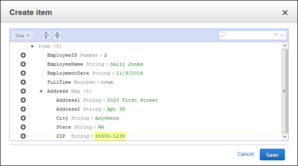
FIGURE 12-16: Complex data appears as indented entries.
It isn’t apparent from the figure, but you use a slightly different technique to work with attributes in this case. When you want to add a new attribute, one that’s at the same level as the map, you actually click the plus sign (+) next to the map entry, which is Address in Figure 12-16. However, if you want to add a new entry to the map, you must click the + next to one of the map entries, such as Address1.
Modifying items
Several methods are available for modifying items. If you want to modify all or most of the entries in the item, select the item’s entry in the list and choose Actions ⇒ Edit. You see a dialog box, similar to the one shown in Figure 12-16, in which you can edit the information as needed. (If the information appears with just the complex data shown, click the Expand All Fields button at the top of the dialog box.)
To modify just one or two attributes of an item, hover your mouse over that item’s entry in the Items tab. Attributes that you can change appear with a pencil next to them when you have the mouse in the correct position. Click the pencil icon, and you can enter new information for the selected attribute.
Copying items
You may have two items with almost the same information, or you might want to use one of the items as a template for creating other items. You don’t need to perform this task manually. Select the item you want to copy and choose Actions ⇒ Duplicate in the Items tab. You see a Copy Item dialog box that looks similar to the dialog box shown in Figure 12-16. Change the attributes that you need to change (especially the primary key, sort key, and secondary indexes) and click Save to create the new item. This approach is far faster than duplicating everything manually each time you want to create a new item, especially when you have complex data entries to work with.
Deleting items
To remove one or more items from the table, select each item that you want to remove and then choose Actions ⇒ Delete. DynamoDB displays a Delete Items dialog box, which asks whether you’re sure about removing the data. Click Delete to complete the task.
Deleting a table
At some point, you may not want your table any longer. To remove the table from DynamoDB, select the name of the table you want to remove and then choose Actions ⇒ Delete Table in the Tables page. DynamoDB displays a Delete Table dialog box that asks whether you’re sure you want to delete the table. Click Delete to complete the action.
As part of the table deletion process, you can also delete all the alarms associated with the table. DynamoDB selects the Delete All CloudWatch Alarms for This Table entry in the Delete Table dialog box by default. If you decide that you want to keep the alarms, you can always deselect the check box to maintain them.
Performing Queries
Finding data that you need can become problematic. A few records, or even a few hundred records, might not prove to be much of a problem. However, hundreds of thousands of records would be a nightmare to search individually, so you need to have some method of finding the data quickly. This assistance comes in the form of a query. DynamoDB actually supports two query types:
- Scan: Uses a filtering approach to find entries that match your criteria
- Query: Looks for specific attribute entries
The examples in this section employ two test entries in the TestDB table. The essential entries are the EmployeeID, EmployeeName, and EmploymentDate attributes, shown here:
|
EmployeeID |
EmployeeName |
EmploymentDate |
|
1 |
George Smith |
11/11/2016 |
|
2 |
Sally Jones |
11/09/2016 |
The two methods of querying data have advantages and disadvantages, but what you use normally comes down to a matter of personal preference. The following sections describe both approaches.
Using a scan
Scans have the advantage of being a bit more free-form than queries. You filter data based on any field you want to use. To scan the data, you choose either a [Table] entry that contains the primary key and sort key, or an [Index] entry that sorts the data based on a secondary index that you create, as shown in Figure 12-17.

FIGURE 12-17: Scans employ filters to locate data.
Using a scan means deciding on what kind of filtering to use to get a desired result. The following steps provide you with a template for a quick method of performing a scan (your steps will vary because you need to provide specific information to make the procedure work).
- Choose Scan in the first field.
-
Select either a [Table] or [Index] entry in the second field.
The entry you choose determines the output’s sort order. In addition, using the correct entry speeds the search because DynamoDB will have a quick method of finding the data.
-
Click Add Filter (if necessary) to add a new filter entry.
You can remove filters by clicking the X on the right side of the filter’s entry.
- Choose an attribute, such as in the first Filter field.
- Select the attribute’s type in the second Filter field.
-
Specify a logical relationship in the third Filter field.
This entry can be tricky, especially when working with strings. For example, if you want to find all the entries that begin with the name George, you choose the Begins With entry in this field. However, if you want to find all the employees hired after 11/08/2016, use the > entry instead.
- Type a value for the fourth Filter field, such as George.
-
Click Start Search.
You see the entries that match your filter criteria. You can use as many filters as desired to whittle the data down to just those items you really want to see. Simply repeat Steps 3 through 8 to achieve the desired result.
Using a query
Queries are stricter and more precise than scans. When you perform a query, you look for specific values, as shown in Figure 12-18. Notice that the key value is precise. You can’t look for a range of employment dates; instead, you must look for a specific employment date. In addition, the employment date is a mandatory entry; you can’t perform the query without it. However, you can also choose an optional sort key and add filtering (as found with scans) as well.

FIGURE 12-18: Queries use specific values to find information.
In this way, using a query is more like asking a specific question. You can ask which employees, who were hired on 11/09/2016, have a name that begins with Sally. In this case, you see just one record. Scans can produce the same result by employing multiple filters. The advantage of a query is that it forces you to think in a particular way; also, because you use attributes that are indexed, using a query is faster.