

Integration details
This chapter provides more details about the integration steps that were introduced in Chapter 2, “Integration overview” on page 29.
The following topics are covered in this chapter:
4.1 Integrating IBM Watson Machine Learning Accelerator with Hortonworks
IBM Watson Machine Learning Accelerator integrates with Hortonworks in two ways:
•A remote Spark job can be submitted from a Jupyter Notebook running on an
IBM Spectrum Conductor Spark Instance Group (SIG) to a Hortonworks cluster that has an Apache Livy service running on it. Sparkmagic is used in the notebook to make the connection to Livy.
IBM Spectrum Conductor Spark Instance Group (SIG) to a Hortonworks cluster that has an Apache Livy service running on it. Sparkmagic is used in the notebook to make the connection to Livy.
•Data is read by Spark jobs running on IBM Watson Machine Learning Accelerator by using a Hadoop Distributed File System (HDFS) URL directly or by defining an HDFS connector in IBM Spectrum Conductor.
Apache Livy is a service that enables interaction with a Spark cluster over a REST interface. It supports long-running Spark sessions and multi-tendency. For more information, see Apache Livy - A REST Service for Apache Spark.
Sparkmagic runs in a Jupyter Notebook. It is a set of tools for interactively working with remote Spark clusters through Apache Livy. For more information, see GitHub - Jupyter magics and kernels for working with remote Spark clusters.
One of the major building blocks for running an application on IBM Watson Machine Learning Accelerator is a SIG. Before you create a SIG, you must complete a set of prerequisite steps. For more information about SIGs, see IBM Knowledge Center.
The first step in building an IBM Watson Machine Learning Accelerator cluster is defining a resource group (RG), which contains a set of resources that is part of the IBM Watson Machine Learning Accelerator cluster. RGs provide a simple way of organizing and grouping resources (hosts). Instead of creating policies for individual resources, you create and apply them to an entire group. A cluster administrator can define multiple RGs, assign them to consumers, and configure a distinct resource plan for each group.
RG host lists are defined by a static list or are dynamic. A static list is where you specifically choose which hosts to use. A dynamic list is where you specify either all hosts or a resource requirement so that when new hosts join they are automatically added to the RG.
If you plan to run a GPU-dependent application and have a GPU-based host in the cluster, make them part of the RG too. In this case, create two RGs: one with CPU cores and the other with GPUs.
For the RG with the GPU hosts, ensure that all the hosts in the RG have a number value in the ngpus column and that the number in the Total slots for this group column is equal to the total number of GPUs on all the hosts in the RG. RGs can be static or dynamic by using different host attributes to define membership or by using tags. Resources can be logical entities that are independent of nodes (bandwidth capacity and software licenses). Those resources are used by consumers.
A consumer is a logical structure that creates the association between the workload demand and the resource supply. Consumers are organized hierarchically into a tree structure to reflect the structure of a business unit, department, projects, and so on. You create a consumer and assign a set of RGs to it.
Consumers also help set up different roles for different users to use the resources as needed, and have demarcated differences between them. For example, two departments in an organization (sales and finance) can run different Spark applications for their individual needs with different sets of resources. There can also be resources that can be shared among the different departments based on their business requirements.
4.1.1 Running remote Spark jobs with Livy
This section shows how to run a job remotely on a Hortonworks Spark cluster by using Apache Livy and Sparkmagic. Figure 4-1 shows an IBM Watson Machine Learning Accelerator Jupyter Notebook that uses Sparkmagic to connect to the Apache Livy service running on an HDP edge node.

Figure 4-1 IBM Watson Machine Learning Accelerator with Hortonworks and Livy
On the Hadoop side, install Livy2 on an edge node, which is a node that includes the Hadoop clients for Spark, Hive, and HDFS. The Hadoop distribution vendors typically have detailed documentation about how to accomplish this task. For Hortonworks Data Platform (HDP) V2.6.5, we followed the instructions that are found at Installing Livy - Hortonworks Data Platform.
Install a custom Jupyter Notebook with Sparkmagic on IBM Watson Machine Learning Accelerator by following the instructions that are found in Appendix B, “Installing an IBM Watson Machine Learning Accelerator notebook” on page 121.
The following example uses the Spark MLLib binomial logistic regression code sample from Classification and regression - Spark 2.2.0 Documentation. In this case, we use a different data set for the data that is accessed from HDFS.
Logistic regression is a machine learning (ML) method that is used to describe data and explain the relationship between one dependent binary variable and one or more nominal, ordinal, interval, or ratio-level independent variables.
Criteo is a data set about an ad click-through rate. It contains data about users and the pages they are visiting and calculates the probability that they click certain ads. The data that is used in this example consists of a portion of Criteo's traffic over 7 days. Each row corresponds to a display ad that is served by Criteo. Positive (clicked) and negatives (non-clicked) examples were subsampled at different rates to reduce the data set size. The examples are chronologically ordered.
To install the data into HDFS, run the following commands on one of the nodes in the Hadoop cluster:
•wget https://s3-us-west-2.amazonaws.com/criteo-public-svm-data/criteo.kaggle2014.svm.tar.gz
•tar -xzvf criteo.kaggle2014.svm.tar.gz
•hdfs dfs fs -put criteo.kaggle2014.svm <TARGET DIRECTORY>
In our sample, the target directory is /user/user1/dataset.
Example 4-1 shows the Spark MLlib code running remotely on the Hadoop cluster and reading the data from the HDFS file system. This is an example of data locality, that is, running the application close to where the data is.
Example 4-1 Code snippet to perform logistic regression by using Sparkmagic
%load_ext sparkmagic.magics
%spark add -s test -l python -u http://129.40.2.75:8999 -a u -k
%%spark
from pyspark.ml.classification import LogisticRegression
# Load training data from HDFS
training = spark.read.format("libsvm").load("/user/user1/datasets/criteo.kaggle2014.test.svm")
%%spark
# Create a logistic regression model
lr = LogisticRegression(maxIter=10, regParam=0.3, elasticNetParam=0.8)
# Fit the model training data using the model
lrModel = lr.fit(training)
# Print the coefficients and intercept for logistic regression
print("Coefficients: " + str(lrModel.coefficients))
print("Intercept: " + str(lrModel.intercept))
4.1.2 Accessing the Hadoop data from IBM Watson Machine Learning Accelerator
Figure 4-2 shows a Spark job running on an IBM Watson Machine Learning Accelerator Jupyter Notebook accessing data on a Hadoop cluster. There are a couple options for reading HDFS data in IBM Watson Machine Learning Accelerator: It can be read into a Spark data frame directly by using HDFS URL or by defining an HDFS connector. The latter option includes options for Kerberos.

Figure 4-2 Hadoop data access from IBM Watson Machine Learning Accelerator
In the following example, we reuse the logistic regression example with the Criteo data set. The model runs locally on IBM Watson Machine Learning Accelerator with the data coming from the remote Hadoop cluster.
Example 4-2 shows the Spark reading of the data by using the HDFS URL.
Example 4-2 Code snippet to perform logistic regression by using remote data
import time
from pyspark.ml.classification import LogisticRegression
# Load training data from the remote Hadoop cluster
training = spark.read.format("libsvm").load("hdfs://ib-hdprb001.pbm.ihost.com:8020/user/user1/datasets//criteo.kaggle2014.test.svm")
# note sure if this analysis makes any sense with this type of data
lr = LogisticRegression(maxIter=10, regParam=0.3, elasticNetParam=0.8)
# Fit the model
lrModel = lr.fit(training)
# Print the coefficients and intercept for logistic regression
print("Coefficients: " + str(lrModel.coefficients))
print("Intercept: " + str(lrModel.intercept))
# We can also use the multinomial family for binary classification
mlr = LogisticRegression(maxIter=10, regParam=0.3, elasticNetParam=0.8, family="multinomial")
# Fit the model
mlrModel = mlr.fit(training)
An HDFS data connector can be defined by updating the IBM Watson Machine Learning Accelerator SIG configuration. The SIG must be stopped to make configuration changes. The SIG details include a pane for defining data connectors.
Figure 4-3 shows the data connector pane. Click Add to define the data connector.

Figure 4-3 Adding a data connector in an IBM Watson Machine Learning Accelerator SIG
Provide a name, type, and access URI for the new data connector. Figure 4-4 shows details for the new data connector.

Figure 4-4 New Data Connector details
To use the new connector, save it, redeploy it, and start the SIG. The portion of the notebook that reads the remote data into a Spark data frame can now specify the location directly without the HDFS URL, as shown in Example 4-3.
Example 4-3 Loading data by using an HDFS connector
# Load training data from the remote Hadoop cluster
training = spark.read.format("libsvm").load("/user/user1/datasets//criteo.kaggle2014.test.svm")
This section covered IBM Watson Machine Learning Accelerator integration with Hadoop. We showed how to run a Spark job on the Hadoop cluster by using Sparkmagic in a notebook and how to read HDFS data into a local Spark job.
4.2 Integrating IBM Watson Studio Local, IBM Watson Machine Learning Accelerator, and Hadoop clusters
This section shows how to integrate IBM Watson Studio Local with IBM Watson Machine Learning Accelerator and Hadoop clusters.
Figure 4-5 illustrates the interaction architecture between IBM Watson Studio Local and
IBM Watson Machine Learning Accelerator. Livy is installed as an application on IBM Watson Machine Learning Accelerator and Sparkmagic is used in a IBM Watson Studio Local notebook to create a connection for Spark job execution on IBM Watson Machine Learning Accelerator.
IBM Watson Machine Learning Accelerator. Livy is installed as an application on IBM Watson Machine Learning Accelerator and Sparkmagic is used in a IBM Watson Studio Local notebook to create a connection for Spark job execution on IBM Watson Machine Learning Accelerator.

Figure 4-5 IBM Watson Studio Local with IBM Watson Machine Learning Accelerator
To integrate IBM Watson Studio Local notebooks with IBM Watson Machine Learning Accelerator, install a Livy application on the IBM Spectrum Conductor SIG, as described at the cws-livy GitLab project.
Here are the application installation step details:
1. From the IBM Spectrum Computing Cluster Management Console, click Workload → Application Instances, and then click New to register an application, as shown in Figure 4-6.

Figure 4-6 Registering a new application instance
2. In the New Application Instance dialog, click Browse to select the Livy_0.5.0.yaml application template file that was downloaded from the cws-livy GitLab project, as shown in Figure 4-7.

Figure 4-7 Specifying the application template
3. Next, you are guided through the New Application wizard:
a. For the application instance name, specify Livy2, as shown in Figure 4-8.

Figure 4-8 Specifying an application name
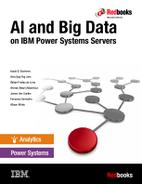
b. For Consumer, select the one that is associated with the SIG. In this case, we had a SIG called Notebook and the consumer has the same name, as shown in Figure 4-9.
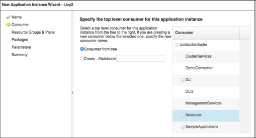
Figure 4-9 Specifying the top-level consumer for the application
c. For Resource Group and Plans, select the resource that you used for the Spark master in the SIG definition. The resources are usually the computer hosts, as shown in Figure 4-10. The Resource Groups and Plans selection box might not appear until you hover the cursor over the location.

Figure 4-10 Selecting the resource groups
d. For the repository package, specify livy_0_5_0_pacage.tar.gz, which was downloaded from the cws-livy GitLab project, as shown in Figure 4-11.

Figure 4-11 Specifying the repository packages
e. Specify the parameter values. For the port number, 8998 is a typical default. If you install the Livy application on multiple SIGs, you need a unique port number for each SIG.
The deployment directory should be unique. We used the deployment directory of the SIG and added /livy2 to it.
The execution user should be the same as the one that you selected for your SIG. If the SIG was built by using the IBM Spectrum Conductor Deep Learning Impact template, the execution user is the ego admin user, typically called egoadmin. For our test, we used an OS user who is called demouser to run the SIG.
The SPARK_HOME and Spark Master URL details can be found in the associated SIG. For our test, we had a Notebook SIG defined. We went to the list of SIG list by clicking Workload → Spark → Spark Instance Groups. Then, we selected the Notebook SIG to see the details for the Spark Deployment and Master URL. For an example the parameters, see Figure 4-12.

Figure 4-12 Specifying the parameter values associated with the SIG
f. The last window of the wizard provides a summary of the inputs. Click Register. It can take several minutes for the application registration to complete.
g. Click Done to exit the wizard after the application instance successfully registers.
The application now is in a Registered state, as shown in Figure 4-13.

Figure 4-13 The Livy2 application in the Registered state
h. Select the check box in the Livy2 application row and click Deploy. You do not need to provide a timeout value in the deploy question message box, so click Deploy again.
i. After deployment completes, select the check box in the Livy application row and click Start. Click Start again in the start question box.
j. Once started, the application has a green Service Summary and shows the URL for the Livy2 application, as shown in Figure 4-14. The URL is what you need to specify in the IBM Watson Studio Local notebook that connects to Livy by Sparkmagic.

Figure 4-14 The started Livy2 Application showing the URL in the outputs
On IBM Watson Studio Local, create a notebook to test the connection to the Livy service by completing the following steps:
1. In the first notebook cell, load the Sparkmagic extension by running the following command:
%load_ext sparkmagic.magics
2. In the second notebook cell, create a Livy session to the IBM Watson Machine Learning Accelerator SIG by running the following command. Use the URL that you obtained while creating the Livy application instance.
%spark add -s <session_name> -l python –u <livy_URL> -a u –k
3. In the third notebook cell, run Spark code in the notebook by running the magic %%spark –l <language> command, where the language for the Livy session is either Python, Scala, or R. The default language is Python. In our example, we used the Spark Context (sc) to create a distributed collection of a 1000 elements and then counted the elements (ans: 1000).
%%spark
sc.parallelize(range(1000)).count()
4. After the application run completes, clean up the Livy session to release the associated resource by running the following command:
%spark cleanup
The ran test is show in Figure 4-15.

Figure 4-15 The IBM Watson Studio Local to IBM Watson Machine Learning Accelerator Livy Notebook Test
After the Livy connection is verified, more sophisticated deep learning (DL) models can be run. Example 4-4 shows the TensorFlow Keras Fashion MNIST model running on IBM Watson Machine Learning Accelerator from an IBM Watson Studio Local notebook. The Fashion MNIST example is described in the TensorFlow basic classification documentation.
The In [#]: prefixes represent the Jupyter Notebook cell numbers in which the code is run.
Example 4-4 Running the TensorFlow Keras model
In [1]: %load_ext sparkmagic.magics
In [2]: %spark add -s test -l python -u http://icpc2.rch.stglabs.ibm.com:8998 -a u -k
In [3]: %%spark
# TensorFlow and tf.keras
import tensorflow as tf
from tensorflow import keras
# Helper libraries
import matplotlib.pyplot as plt
print(tf.__version__)
In [4]: %%spark
fashion_mnist = keras.datasets.fashion_mnist
(train_images, train_labels), (test_images, test_labels) = fashion_mnist.load_data
()
In [5]: %%spark
class_names = ['T-shirt/top', 'Trouser', 'Pullover', 'Dress', 'Coat',
'Sandal', 'Shirt', 'Sneaker', 'Bag', 'Ankle boot']
print("train images shape: ", train_images.shape)
print("train labels count: ", len(train_labels))
In [6]: %%spark
print("test images shape: ", test_images.shape)
print("test labels count: ", len(test_labels))
In [7]: %%spark
train_images = train_images / 255.0
test_images = test_images / 255.0
In [8]: %%spark
model = keras.Sequential([
keras.layers.Flatten(input_shape=(28, 28)),
keras.layers.Dense(128, activation=tf.nn.relu),
keras.layers.Dense(10, activation=tf.nn.softmax)
])
model.compile(optimizer=tf.train.AdamOptimizer(),
loss='sparse_categorical_crossentropy',
metrics=['accuracy'])
model.fit(train_images, train_labels, epochs=5)
test_loss, test_acc = model.evaluate(test_images, test_labels)
print('Test accuracy:', test_acc)
In [9]: %%spark
predictions = model.predict(test_images)
predictions[0]
In [10]: %spark cleanup
In [11]: #@title MIT License
#
# Copyright (c) 2017 François Chollet
#
# Permission is hereby granted, free of charge, to any person obtaining a
# copy of this software and associated documentation files (the "Software"),
# to deal in the Software without restriction, including without limitation
# the rights to use, copy, modify, merge, publish, distribute, sublicense,
# and/or sell copies of the Software, and to permit persons to whom the
# Software is furnished to do so, subject to the following conditions:
#
# The above copyright notice and this permission notice shall be included in
# all copies or substantial portions of the Software.
#
# THE SOFTWARE IS PROVIDED "AS IS", WITHOUT WARRANTY OF ANY KIND, EXPRESS OR
# IMPLIED, INCLUDING BUT NOT LIMITED TO THE WARRANTIES OF MERCHANTABILITY,
# FITNESS FOR A PARTICULAR PURPOSE AND NONINFRINGEMENT. IN NO EVENT SHALL
# THE AUTHORS OR COPYRIGHT HOLDERS BE LIABLE FOR ANY CLAIM, DAMAGES OR OTHER
# LIABILITY, WHETHER IN AN ACTION OF CONTRACT, TORT OR OTHERWISE, ARISING
# FROM, OUT OF OR IN CONNECTION WITH THE SOFTWARE OR THE USE OR OTHER
# DEALINGS IN THE SOFTWARE.
tf_fashion_minst_paie_livy.jupyter http://localhost:8888/nbconvert/html/redbook-watson-studio-local/tf...
2
4.3 Integrating IBM Watson Studio Local with Hortonworks Data Platform
Figure 4-16 illustrates a typical interaction architecture between IBM Watson Studio Local and HDP.

Figure 4-16 IBM Watson Studio Local with Hortonworks
IBM Watson Studio Local provides a Hadoop registration service that eases the setup of an HDP cluster for IBM Watson Studio Local. Using Hadoop registration is the preferred approach because it provides more functions for scheduling jobs as YARN applications.
To integrate IBM Watson Studio Local with HDP, complete the following steps:
1. Install the DSXHI (Hadoop registration gateway service and Hadoop registration rest service) in one of the edge nodes of the HDP by using the steps that are detailed in
IBM Knowledge Center.
IBM Knowledge Center.
2. On the IBM Watson Studio Local browser, click Admin Console → Hadoop Integration.

Figure 4-17 Add Registration window
Adding the registration integrates IBM Watson Studio Local with the HDP nodes for remote Spark job submission.
4. After registration is complete, you can view details about the registered Hadoop cluster, push runtime images to the Hadoop cluster, and work with images. For more information, see Hadoop Integration.
5. After the runtime environment push completes, use a IBM Watson Studio Local notebook to work with the Hadoop cluster. Example 4-5 shows the import of the dsx_core_utils package and the call to dsx_core_utils.get_dsxhi_info().
Example 4-5 Notebook code to get the list of Hadoop clusters
import dsx_core_utils
DSXHI_SYSTEMS = dsx_core_utils.get_dsxhi_info(showSummary=True)
The result of the get_dsxhi_info call shows a list of the Hadoop clusters, type of service (livyspark2), and the image ID names. Example 4-6 shows how the result appeared on our test system.
Example 4-6 List of available Hadoop systems
Available Hadoop systems:
systemName LIVYSPARK LIVYSPARK2 imageId
0 pw8002 livyspark2 dsx-scripted-ml-python2
1 pw8002 livyspark2 dsx-scripted-ml-python3
2 pw8002 livyspark2 py-tqdm-1.0-dsx-scripted-ml-python2
3 pw8002 livyspark2 tensorflow-1.12-dsx-scripted-ml-python3
4 pw8002 livyspark2 tf-numpy-1.12-dsx-scripted-ml-python3
6. You can configure the Spark session that is when running on the selected registered Hadoop Integration system. Example 4-7 shows an example configuration.
Example 4-7 Configuring a Spark session
myConfig={
"queue": "default",
"driverMemory": "2G",
"numExecutors": 2
}
7. Run dsx_core_utils.setup_livy_sparkmagic to set up Sparkmagic to connect to the selected Hadoop Integration System, as shown in Example 4-8.
Example 4-8 Setting up Sparkmagic
# Set up sparkmagic to connect to the selected registered HI
# system with the specified configs. **NOTE** This notebook
# requires Spark 2, so you should set 'livy' to 'livyspark2'.
dsx_core_utils.setup_livy_sparkmagic(
system="pw8002",
livy="livyspark2",
imageId="dsx-scripted-ml-python2",
addlConfig=myConfig)
# (Re-)load spark magic to apply the new configs.
%reload_ext sparkmagic.magics
8. Create a remote Livy session to connect to that Hadoop Integration System by using the following command:
%spark add -s <session> -l python –u <livy_URL> -a u –k
Example 4-9 shows the command to connect to our test HDP cluster.
Example 4-9 Starting the remote Livy session
session_name = 'tfsess1'
livy_endpoint = 'https://ib-hdprb001.pbm.ihost.com:8443/gateway/p460a10/livy2/v1'
webhdfs_endpoint = 'https://ib-hdprb001.pbm.ihost.com:8443/gateway/p460a10/webhdfs/v1'
%spark add -s $session_name -l python -k -u $livy_endpoint
A successful start shows a table that includes the Livy session ID and the YARN application ID for pyspark.
Any cell in the notebook that has %%spark as its first line runs the job remotely on the Hadoop system.
You can access any data from the HDFS file system by using functions like spark.read.format() to read the data frames from the file system.
Example 4-10 shows a Spark MLlib sample run.
Example 4-10 Running Spark on the Hadoop cluster from the IBM Watson Studio Local notebook
%%spark
from pyspark.ml.classification import LogisticRegression
# Load training data
training = spark.read.format("libsvm").load("data/mllib/sample_libsvm_data.txt")
lr = LogisticRegression(maxIter=10, regParam=0.3, elasticNetParam=0.8)
# Fit the model
lrModel = lr.fit(training)
# Print the coefficients and intercept for logistic regression
print("Coefficients: " + str(lrModel.coefficients))
print("Intercept: " + str(lrModel.intercept))
9. Clean up the remote Livy session by running the following command, which terminates the session and releases resources back to the remote Hadoop Integration system:
%spark cleanup
Image customization
IBM Watson Studio Local uses containers to manage the complete lifecycle of the images of the applications, which provide the complete benefits of containers to the IBM Watson Studio Local environment.
IBM Watson Studio Local supports creating custom images and pushing those images to systems that are registered through Hadoop Integration.
To customize an environment by using the Python tqdm library complete the following steps. This process can be extended to other packages.
1. Start the environment.
From your project home page, use the Environments tab to start a Jupyter with Python 2.7 environment if it is not already running (a green dot indicates that the environment is running).

Figure 4-18 Starting the environment
2. Install the package by using the environment’s terminal.
From your project home page, use the Environments tab to start a terminal shell for the environment that you started in step 1 on page 82.
When you are inside the terminal, run the following command to install tqdm:
conda install tqdm -y
When the command completes, you can exit the terminal, as shown in Figure 4-19.

Figure 4-19 Installing the package
3. Save the environment as a custom image.
From your project home page, use the Environments tab to save the environment that you edited in step 2 on page 82.

Figure 4-20 Saving the image

Figure 4-21 Selecting Hadoop Integration from the admin console
5. Display the details, as shown in Figure 4-22.

Figure 4-22 Displaying the details of the registered Hadoop system
6. Push the run time to the Hadoop cluster, as shown in Figure 4-23.

Figure 4-23 Pushing the run time
7. Select the new image in the notebook.
The Hadoop Integration utilities provide a list of images that can be used when connecting to the Hadoop cluster. Select the image to use when connecting to the cluster.
Working with Hadoop data
IBM Watson Studio Local supports the addition of many data sources and remote data sets, including Hive and HDFS for Hadoop clusters. For more information, see Add data sources and remote data sets.
You can shape and refine the data sets by using the Data Refinery.
..................Content has been hidden....................
You can't read the all page of ebook, please click here login for view all page.