Chapter Three

Numbers, Expressions, Functions; Rocket Golf Near Lightspeed

Note to Instructor: This problem, as stated, requires the same level of relativity as covered in elementary physics texts and is thus appropriate for first- or second-year college students. Even if the students do not understand the full implications of the two equations we use, (3.4) and (3.5), it is their application that is the point of this chapter. However, it is conceptually challenging to go further and ask about the golf ball’s trajectory as viewed in different frames, as this involves the questions of simultaneity and acceleration in relativity.

3.1 PROBLEM: VIEWING ROCKET GOLF

Michele, a golf fanatic, would like to break the world’s record for the fastest golf ball hit. Money being no object, she rents a rocket and hits her golf balls from the moving rocket. The rocket is fast, with a speed of c/2, where c is the speed of light (299 792 458 m/s). (This really is fast considering that no object with mass can attain a velocity of c.) As indicated in Figure 3.1, Michele hits her drive with a speed of , at an angle θ = 30, as she measures with respect to the moving rocket. She observes her drive to remain in the air for a hang time T’ = 2.6 × 10⁷ seconds (which is almost a year!). Ben, an observer on the earth, sees her rocket moving to the right with a velocity v = c/2, and this velocity somehow gets added to that of Michele’s golf ball.

Figure 3.1 Observer Ben on Earth watching Michele on a rocket hitting a golf ball. Ben is at rest in frame O on the left and Michele is moving to the right with velocity v (horizontal arrow) in Frame O’. Michele sees her golf ball hit with velocity U’.

Problem a: Since some readers may not be familiar with special relativity, we do not expect you to solve this problem on your own, or even to understand all the equations. Although the theory of special relativity does have it subtleties and fine points, it is accessible to beginning students and we will use only a few simple results. We will lead you through the solution for two cases and then ask you to follow our steps for a third case. This should give you a good working knowledge of some tools (the main focus of this chapter). The third case you work out is the interesting one in which round-off error arising from the use of floating-point numbers (“floats” or “doubles”) becomes evident. Usually it takes many computational steps before you see the effect of round-off error, but in this problem it arises fairly simply. Your explicit problem is:

3.2 THEORY: EINSTEIN’S SPECIAL RELATIVITY

Being told that an object is traveling with a velocity near that of the speed of light is a hint that the problem is not a simple mechanics one. Indeed, this means that we need to apply Einstein’s special theory of relativity [Smith 65, Ser 00] to it. As indicated in Figure 3.1, we start by considering Ben in a reference frame O with axes (x, y) attached to the earth, and Michele in frame O’ with axes (x’, y’) attached to the moving rocket. Relative to Ben, frame O’ (the rocket) is moving along the positive x axis with uniform velocity v. Likewise, Michele feels herself at rest in the rocket and sees Ben moving to the left with velocity —v. Both are equally correct and agree on their relative velocity; indeed, this is the reason it is called the theory of relativity.

Ben and Michele may agree on their relative velocities, but they do not agree on measurements of times and distances. As an example, if Michele says that her golf ball was in the air for a period of time T’, then Ben will say that the ball was in the air for a longer time

where γ is a function of relative velocity v that is always greater than 1:

In view of the fact that the speed of light c is so much larger than any velocities we normally encounter, γ is usually very close to 1 and only gets large for exceedingly high velocities (normally restricted to elementary particles). The fact that Ben would measure a longer hang time than Michele is called time dilation and is often described with the phrase “moving clocks run slow.”

The additional result we need from special relativity relates the velocities seen by Michele and Ben. If Michele in the moving rocket O’ sees her golf ball having velocity components

then Ben on earth O, will see her golf ball move with velocity components

where γ is the function (3.2) as before. If you study (3.4) a bit, you will notice that the numerator describes the usual addition of relative velocities, while the denominator is the relativistic correction. In turn, the relativistic effects are in the numerator of (3.5).

3.3 MATH: INTEGER, RATIONAL AND IRRATIONAL NUMBERS

There are different types of numbers that are used in mathematics and in computation. For instance, there is a countable infinity of integers, 0, 1, 2, 3,…, and nearly twice that many if we also include negative integers. Maple stores these integers exactly and tries to retain infinite precision for its pure mathematical operations with them. Yet while a computer program may be smart, the computer is finite and sooner or later it will run out of room if we try to compute with very large numbers that are stored exactly. For this reason computers often store very large (and very small) numbers approximately, using the floating-point representation, a variation of scientific notation. We shall discuss that soon.

Even though the number of integers is infinite, there is a yet larger infinity of rational numbers, namely, of numbers formed by the ratio of two integers, N/D. Maple stores these rational numbers exactly, by storing the numerator and denominators as integers and then displaying a fraction rather than a bunch of digits. To see what this means in action, enter these operations and interpret the results:

1/3; 4/2; 2485/3479; 3(1/3); 3 * (1/3);

After the Maple prompts we obtain:¹

1/3  2  5/7  3  1

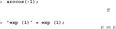
There are also numbers in our world that cannot be expressed as the ratio of integers, and so would require an infinite number of digits to store. These are called irrational numbers and include numbers like π or e (the base of natural logarithms). When Maple encounters irrational numbers, it usually uses the familiar symbol for them rather than approximating them by a fraction or a decimal. By way of example, see what happens when you ask Maple to use some of its built-in functions to determine the angle whose cosine is –1, or raise e to the first power:

These results are more than pretty symbols. Maple knows the meaning of these and other symbols, as seen from the response to log(%). Here the percent sign % means “the previous expression,” and %% means the one before that. Try it:

Maple understands more than just symbols, it actually knows an incredible amount about a myriad of functions, too. Some common ones are

ln(x), log10(x), abs(x), cos(x), sin(x), sqrt(x), arcsin(x), cosh(x).

Others are given in an Appendix B or found under Maple’s Help menu. Now and then you will need to include π or e, or some other irrational, into one of your commands. Maple normally accepts expressions like pi, Pi, PI, e, or E as algebraic symbols. You may always define these symbols to be what you want (with techniques that we will get to shortly), but Maple has predefined many such symbols for general use.

So, now we prompt you to run Maple and deduce what it thinks of each. You should have found that cos(pi) and cos(PI) produce nice output, since Maple recognizes pi and PI as lower- and uppercase Greek letters. However, they are treated like any other algebraic symbol and do not have values associated with them (unless you have assigned values to them, of course). In contrast, Maple recognizes Pi as the ratio of the circumference to the diameter of a circle and evaluates cos(Pi) = -1 just fine. However, we do have to input the rather inelegant exp(1) to get the mathematical e (this was not true in previous versions of Maple and may well change again).

3.4 CS: FLOATING-POINT NUMBERS

In spite of integers being neat to work with, there are limits to the kind of calculations possible with them. Occasionally you might want to see what the numerical value of an irrational number like π or sin(1) is, or you may need to deal with a really large number, like the size of the universe. Numbers with decimal points are stored on the computer in a format known as floating-point notation or real. This notation is similar to scientific or engineering notation of the form

mantissa × 2 ^exponent

The term “floating-point” denotes the idea that the decimal (or binary) point moves around or “floats” during calculations in order to keep the number of digits in the mantissa constant.

One easy way to tell Maple that you want to do some work using floatingpoint numbers (“floats”) is to place a decimal point in one of the numbers of your calculation. This automatically makes it a floating-point number, and if one of your numbers is a float, Maple often assumes that you want all the other numbers to be as well. To experience this in action, enter and observe Maple’s response to each of the following (we give answers here):

The other way to get Maple to do a calculation using floats or reals is to explicitly tell it to evaluate some expression as a floating-point number. This is done with the evalf function or command (the f means “float”):

If you count the number of 3’s in the first case, you will see that Maple has stored 10 decimal places (the word length). This is the default value and is about as good as a pocket calculator. Actually, there is a variable internal to Maple called Digits that determines this number of significant figures, and it is usually set to 10. You may change the value of Digits quite easily if you want more or less precision:

3.4.1 Powers of 10

We have just seen how Maple stores numbers in floating-point or scientific notation. Unless you are dealing with an exact power of 2, like 256, this floating-point representation of a number is always approximate, since only a finite number of digits is used to store the mantissa. In the course of discussing exponents and exponentials, which are related but different, it is useful to see how to enter a number as a power of ten in Maple.² Enter each of the following with the spacing exactly as given, and explain Maple’s response to each (we give answers here in the printed text):

We deduce from these results that:

3.5 COMPLEX NUMBERS

A complex number is the sum of a real number and an imaginary number. An imaginary number is times a real number.³ Usually mathematicians and physicists use the symbol i to represent , while engineers often use the symbol j; regardless of its name, it is the same number, and it does not really exist in our world. Maple, in turn, marches to its own drummer and uses I to represent . To see how this works (we will encounter complex numbers in a number of places again), we give you some examples:

3.6 EXPRESSIONS

We started our work with Maple by using it as an expensive pocket calculator. You key in commands one at a time and Maple evaluates them one at a time. Maple does much more. One of the truly unique things it does is mathematics, including calculus, with algebraic symbols. Many of the commands in Maple work with either numbers or symbols. We shall see some examples of that.

In a semantic sense, most of the commands that we have so far given to Maple are expressions and statements. Whereas you may know what these terms mean in common English, they have rather specific meanings in both computer science and mathematics.⁴ Expressions are objects that have numerical values (or would have values if the variables contained in them had values). Commands like 1+4; and sin(Pi/2) are expressions with values 5 and 1 respectively. On the other hand, exp(x)-1 is also an expression, but it has a numerical value only if x has previously been assigned a value. Try it:

Observe, when Maple just echoes what you entered, it is being diplomatic and telling you that it heard what you have said but cannot do anything about it. If you want more, then you need to tell it more!

3.6.1 restart and unassign

When we refer to a constant, we mean an object whose value does not change. As an instance, PI = π is such a constant. When we refer to a variable, we mean a data item whose value may change. For example, the circumference C = 2 * PI * r will have different values depending upon the radius r of the circle. When we refer to a symbol, such as x, we view it as one would in algebra; namely, as an abstract object representing something more concrete. Sometimes x may have a numerical value, and at other times it may not. In either case we may manipulate it using the rules of algebra and calculus.

When a symbol has been assigned within a worksheet, it normally stays assigned until you change it or until you close that particular worksheet. (It is often useful to have several worksheets open at one time, possibly even different versions of the same worksheet.) Every so often you may be happily working away or editing deep within a worksheet that was working just fine for you, and for some reason your statements no longer appear to be working correctly. The problem may be that you have forgotten that some variable has been assigned previously, and you are using it as if it had not been. That being the case, you need to unassign the variables. Also, if you just jump into the middle of a worksheet, you do not know that variables have been assigned or that packages have been called, in which case it would be safest to “start with a clean slate.” If Maple really seems to be working improperly, you should save your files, exit Maple, and then start it again.

To start again with all new variables as if it were a whole new session:

Unless you have reason not to, it is a good idea to issue the restart command at the beginning of each new group of operations.

To unassign a single variable, use single quotes to assign that variable back to a literal or symbolic version of itself, or use the unassign command:

3.6.2 Exercise (How Expressions Are Stored)

The factorial operation n! = n(n-1)(n-2) • • • (2)(1) occurs frequently in mathematics. If n is an integer, then Maple evaluates n! just as you would expect. Run Maple to determine what is the ratio of (1001)! to 1000!:

However, when n is a symbolic variable with no value assigned to it, Maple prefers to store it as n! rather than as the product of many terms. This makes sense because it saves memory and because it makes further manipulations easier:

It may appear that Maple is arrogantly repeating to you the command that you have just issued, yet a more understanding view is that Maple does not think like you and so has to be told more explicitly just what you have in mind. In this case, Maple has worked out an answer that apparently looks fine to it, while we might prefer something simpler. So we tell Maple to simplify the answer:

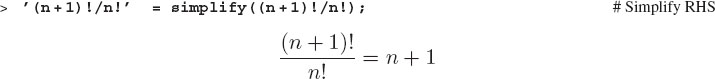
Exercise: Calculate the ratio of (n + 50)! to n!, remembering to simplify. Calculate the ratio of (n+m)! to n!, where n and m are algebraic. (Maple may output Γ for the gamma function. This is the correct answer. You would have to tell Maple that m and n are integers to get m! as the answer.)     ♠

3.7 ASSIGNMENT STATEMENTS

indexStatements

Whereas expressions have values, statements cause things to happen. In other words, statements have side effects, such as assigning values to variables or plotting up some graphs. The most common sort of statement is the assignment statement setting one object equal to another:

We see that the side effects of these statements are that Digits (which determines the precision of floating-point calculations) will subsequently have the value 4, and that x will have the value 0.3333.

Because assignment statements set things equal to each other, they must contain an equal sign. The equal sign: = with a colon in front is called an assignment operator. It may be thought of as saying “set the variable on my left equal to the value on my right.” To a computer this means “go to the location in memory where the value of the variable on my left is stored, and place the value on my right into that memory location.” In contrast to conventional programming languages, like C or Java, Maple permits the value on the RHS to be purely symbolic.

In spite of the assignment statements above looking like equations, they do not express the same type of equality as algebraic equations. To illustrate, when we say x = y in algebra, we mean that the objects on both sides of the equal sign are the same. Thus it follows that y = x is also true. Yet when we issued the Maple statement Digits: = 4;, we are issuing a command to replace whatever was stored in memory as the value of Digits with the new value 4. What we most certainly do not want, is 4 = Digits; namely, to have all values of 4 replaced by the present value of Digits, which is usually equal to 10. To make it clear that assignment equality is not the same type of equality as in algebra, the: = sign is used instead of the ordinary = equal sign.

On account of computer languages containing two types of equality, you have to exercise some care with your equal signs. To prove the point, if you leave off the colon: Maple does not complain, but the effect is not the same:

Thus we see that when tell Maple Digits = 3;, it just tells us that we are stating that 10 = 3 without resetting the value of Digits. As there are no side effects associated with =, no harm is done, but then again, no good is done either. A more proper use of assignment statements is:

Here we assigned y the value 3 and then assigned x the current value of y. Maple told us that x was assigned the value 3, as expected.

Assignment statements are not limited to numerical values. You are able to assign symbolic values as well:

Now that we have set x equal to y, Maple remembers that y and x are the same, until you assign another value to x.

3.8 EQUALITY (RHS, LHS)

Maple does have a place for the usual = equal sign. In fact, it uses it in its output, for example, when the solution to an equation is given as x=y. Notwithstanding that both sides of an equation are equal to each other, it is often helpful to deal with the left-hand side (LHS) and the right-hand side (RHS) separately:

3.9 FUNCTIONS

Mathematicians and scientists make their work easier by employing functions. Computer scientists do much the same thing with what they also call methods and subroutines, although these latter two are able to do more than a simple function might. Consequently, while we will speak of “functions” in Maple and mathematics, when we get to programming we will speak of “methods,” which is just another name for the same thing.

As visualized in Figure 3.2, a function f(x) may be thought of as a mathematical meat grinder in which you feed in some variables at one end and get out some values of the function at the other end. As a case in point, f(x) = 10x⁴ sin(3 x) is such a function. You feed it the variable x, the function multiplies x by 3, evaluates the sine of 3x, multiplies that by 10x⁴, and then returns the result. In other words, x is the independent variable that we choose, and y = f(x) is the dependent variable.

We know that this may sound familiar to you, but it is worth repeating that the numbers 3 and 10 occur in our function as parameters that are not expected to be changing much. Thus, if we replace these numerical parameters with algebraic symbols f(x) = A x⁴ sin(k x), then x is still the independent variable, and A and k are now the parameters, although they are represented by symbols that take on arbitrary values. Apparently, whether a symbol is a variable or a parameter is determined by its use, which we usually figure out from the context. Therefore we also could write our function as a function of three variables, f(x, k, A) = A x⁴ sin(k x). Functions of more than one variable are called multi-variate functions and are much like our meat grinder in Figure 3.2, except that we now have a number of ingredients.

Figure 3.2 A function as a meat grinder; arguments x and y go in, function f(x, y) comes out.

When we instruct a computer program such as Maple to create a function for us, we have to decide which symbols are variables and which are parameters. As a rule of thumb, it is probably best to base your decision on convenience: if it is unlikely that the values for the parameters will change, then it is simpler and clearer to build them into the function, for example, 3 and 10 in our function. If it is likely that you will want to change the parameters, for example, to create plots, then it is probably best to treat them as variables.

3.9.1 Built-In Functions (List in Appendix B)

Even though mathematical functions occur in descriptions of our world, computers do not inherently know about them. However, there are often collections of programs called libraries that supplement computer languages and contain many functions and methods. Maple has an extensive library of such functions, and we give a complete list in Appendix B, which you can also get as the Maple’s Help menu. Some functions that you may find most useful are:

Most conventional computer languages handle these common functions as would your calculator; you key in a number, you get back a number. In contrast, symbolic languages also know much about the mathematical properties of these functions so that you can also input symbolic values and have them processed.

In its usual insightful manner, if you give Maple a floating-point number as input, it will evaluate the function numerically. If one argument is symbolic, then Maple will return a symbolic answer. We try this with our example:

We see that Maple has remembered the value of x from one line to the next (it actually will remember the value of x until we do something to reassign it or until we enter restart). Regardless of the fact that we entered purely numerical values for the argument of the sine function, Maple has still not given us the answer you would get from a calculator! Do not get annoyed. The answer y = 100000 sin(30) is an exact mathematical expression with no approximations made, and so Maple keeps it that way. If we want a floating-point or decimal number as an answer, then you must force Maple to make the approximation by having it evaluate the answer as a floating-point number:

where we have used the: = on the LHS to get a nice-looking answer. Alternatively, you could have used a floating-point number in the argument of the function, in which case Maple would automatically convert to floats:

Now we try some variations on the preceding commands in which either x is a float, or the factor in front of the sine function is a float:

As we have said before, unless you instruct otherwise, Maple performs all floatingpoint calculations with 10 significant figures.

3.10 USER-DEFINED FUNCTIONS

In addition to Maple’s built-in functions, you can define your own functions and call them anything you want. To name an instance, let us say we want to define the function 10 x4 sin 3x as the function g(x):

Survey a few things here. The LHS of: = contains the name of the function g being defined. The RHS is immediately followed by the argument x of the function and then an arrow pointing to the function definition. Accordingly, if you think of the function g(x) as “gee of ex,” then the g goes to the left of the: = and the x goes to the right. Scrutinize how the arrow sign -> is entered as a minus – followed by the greater-than > sign. Maple responds by showing you this so-called arrow function or mapping in its proper mathematical notation. You then use your function g(x) just like a built-in one. Evaluate g(10) and see if you get the same answer as we did above:

Defining functions of several variables (multivariates) requires you to add some more variables to the argument list. This is a useful way to feed a single-variable function the parameter values it needs. By way of example, to create our old friend y = Ax4 sin(bx) as a function of three variables, we replace (x) with (A,b,x):

3.11 REEXPRESSING ANSWERS

Maple knows that is 4 and will evaluate it with no further ado. However, if there is no exact root to some number, then Maple will reduce the number down as far as it is able but may leave some part of the number in root form. Numbers with explicit ro√ots are called algebraic numbers. For instance, if we ask Maple to evaluate

all we get is a pretty form of what we entered. So we will tell Maple that we would like the expanded form of the previous expression:

There are a bunch of Maple commands, such as

simplify factor allvalues expand value eval collect expand normal

that are useful in getting Maple to change the form of its answers to something you might like better. For example, how about some cute cube roots:

where I is the imaginary number.

As we get into more complicated calculations, we shall see that there is little question that Maple does algebra well. However, the results it gives are not always in a form that humans find revealing. Indeed, learning how to use Maple is more than just learning the names and grammar of a whole bunch of commands, it is also acquiring a trademarked trial-and-error state of mind in which you naturally try to manipulate Maple’s output until it produces the most mathematically revealing form for you. In this section we look at some manipulations and some “tricks.”

Maple is real good at summing finite and infinite series:

This result is not the outcome n(n+1)/2 that we learned in our algebra, so we try to simplify it:

Now we produce some other complicated expressions and try to simplify them:

You see here that expand and factor mean the same things as they do in algebra. The command simplify uses identities and properties of functions to simplify an expression and has a number of advanced forms (read about them in the Help pages). The normal command, on the other hand, is useful for simplifying rational expressions:

3.11.1 Simplifying Examples

3.11.2 Expressions Behaving Like Functions: eval, evaln

It seems perfectly reasonable to think of a variable like x or y as a symbol that does not vary the way functions do. However, Maple is so smart and has such a good memory that if you set a variable equal to a complicated expression, such as polynomial, Maple will treat that variable much as it does the complicated expression and substitute in values for the variables contained in it. Consequently, it should come as no surprise that the manipulations we did on expressions are allowed on variables representing expressions:

(x+12)¹⁵

Even though we are manipulating z as if it were a function, it is not a true function and does get evaluated differently. To cite an instance, if we enter z(3) as if the expression were a function, we get something interesting but not 5¹⁵:

Seeing that we have brought up the eval function, we should also indicate that there is a variant of it called evaln that evaluates a variable to a name. Its purpose is essentially the same as the use of quotes to set a variable back to symbolic form after it has been assigned a numerical value, however it is what is needed if you are dealing with subscripted variables:

3.11.3 Converting Expressions to Functions: unapply

Even though the difference between functions and variables may seem mainly semantic, there are instances where the difference matters. The unapply command is used to convert an expression or variable into a true function. The funny name arises from the idea that we normally “apply” a function to a variable to obtain a value, while here we are working backwards and creating a function from a variable. The unapply command takes an expression and a variable as its two arguments and returns a function of the second argument:

3.12 CS: OVERFLOW, UNDERFLOW, AND ROUND-OFF ERROR

All computers are finite and, alas, Maple is too. This means that if you keep making numbers bigger and bigger, at some point the computer cannot handle them and an overflow exception occurs. Likewise, if you keep making numbers smaller and smaller, at some point an underflow exception occurs. In addition, since floating-point numbers are stored with a finite number of significant figures, the digit beyond the last one is truncated, and the last digit is rounded off. Similarly, if the truncated digit is greater than 5, then the last stored digit is rounded up, and this leads to round-off errors. (For convenience, both truncation and round-off errors are usually called “round-off errors.”) In principle, the algorithms used by Maple for calculations have no limit to their precision and should be exact if no floating-point numbers are called. In practice, Maple uses 524, 279 digits, which should not be too hard to live with, but you may ask for more. Serious problems result if you write a program and underflows or overflows occur within it, or if there is a great deal of round-off error.

Enough talk, let us have some fun and see if we are able to break Maple using the factorial, n! = n(n - 1)(n - 2) • • • (2) (1), and powers of 10. Do not worry, you will do no permanent harm and no one will yell at you if you break Maple, although you may lose the active worksheet. In general, you get no warning that Maple is about to break, so drive defensively and Save Often! If Maple stops responding for a considerable amount of time, it may be working, or it may be stuck. Before you quit or kill Maple, you may want to try the Stop button in the tool bar and see if Maple responds again. Else you have to quit. Here we challenge Maple and show how it admits failure:

Because calculations that employ floating-point numbers are are often truncating or rounding off the last digit in the mantissa, and because these errors tend to accumulate in time, their final results may be less precise than the numbers you input. This is called truncation and round-off error. We use the term “error” here in much the same way one does when speaking about the experimental “error” in a physics laboratory. It is not an error in the sense that you read the meter wrong or had your finger caught in the caliper but is really an uncertainty arising from the finite number of digits used to represent numbers.

To see a living example of round-off error, work through the following commands (we decrease the normal precision to make the effects more evident):

3.13 SOLUTION: VIEWING ROCKET GOLF

Problem a: We will now apply our Maple tools to the relativistic golf-ball problem. Michele on the moving rocket sees her golf ball travel with velocity U’ at an angle θ, with a hang time T’:

Ben on the earth observes the rocket moving with a speed v = c/2. He sees the golf ball with velocity components U^x and U^y and a hang time of T. The equations of special relativity (that we have not derived and that we do not expect you to fully understand) relate Michele’s and Ben’s observations

Because the time dilation function γ(v) is rather complicated and is used in several places, we start our solution by defining a Maple function for it:

Whoops! Although this was the obvious thing to do, it does not work, because Maple apparently has its own function gamma and does not want us to steal its name. On account of this we try defining our function using a capital G:

Ah, that is better. To make life simple for us beginners, let us adopt the convention that we measure all velocities as a fraction of the speed of light c. Thus, rather than saying v = c/2, we would just say v = 1/2. This will make the equations look simpler and save us some time. This being the case, we redefine Gamma as:

This function is apparently acceptable to Maple, but we need to test it before we believe it is right. We know by looking at the equation defining γ(v) that γ(v = 0) = 1, and that γ should get progressively larger as v approaches the speed of light c. So we try:

These appear to be getting larger, but to be sure let us repeat the calculation using floating-point numbers. We do that by acting on the function with the evalf function or just by placing some decimal points in the arguments. We will be lazy:

Yes, γ does grow as v approaches the speed of light. But what happens if the velocity equals the speed of light?

Well this does not tell us much, because division by zero is not defined. However in a mathematical sense we really want the limit as v approaches c in infinitesimal steps, and so we will try the limit command:

Maple clearly has a problem here, and it is telling us that we did not give it a good enough description of what we want. Well, this is a case where precision in mathematical language is called for. The cause of the problem is that there is an infinity at v=1 (a division by 0), and the limit depends on just how we approach that infinity. As told by the Help reference, we need an option to the limit command to indicate that we are approaching the singularity from the left, namely, from v <c:

This is better. We see that the time dilation factor γ approaches ∞ as the rocket speed approaches the speed of light.

We will discuss plotting in more detail in Chapter 4. Nevertheless, we make here a simple plot of γ(v) using Maple’s plot command. Because we have set c = 1, there are no variables with symbolic values in γ(v), and so Maple evaluates it as a number and plots it:

We see that γ(v) is essentially 1 until the velocity gets close to the speed of light. Indeed, this is why we do not usually experience relativistic effects in our everyday lives. For the problem at hand, the exact and floating-point values of γ that we will use are:

The difference in value from 1 indicates that there is a significant relativistic effect for our problem. Specifically, Ben says that the golf ball stayed in the air 22% longer than Michele thought it did:

Next we calculate the speed U that Ben observes the golf ball to have, knowing that Michele says she hit it with velocity U’. We need then to calculate:

where we have assumed all velocities will be entered as a fraction of c, and so v = c/sqrt3. To be flexible, we create functions to calculate these velocity transformations, one of which calls our previously defined Gamma function:

Ben knows Michele’s value for θ, and, after converting it to radians, uses it as input:

If nonrelativistic kinematics are applied to this problem, we would see Michele’s golf ball moving at the combined speeds of the rocket plus its speed relative to the rocket:

Yet relativity teaches us that this is not possible for anything but light. If we look at the answer we just calculated, we see that the velocity seen by Ben is less than c (1 in our units):

Now that we have calculated the components Ux and Uy of the velocity in Ben’s frame, we calculate the angle φ at which Ben sees the golf ball fly off by using the fact that

Inasmuch as the argument to the arctangent function could be infinite if Ux =0, Maple’s arctangent function takes Uy and Ux as separate arguments:

Thus we see that while Michele saw her ball fly up at 30 degrees, Ben sees it “pushed forward” to about 14 degrees.

Problem b: In this version of the problem, we have Michele hitting her golf ball backwards, namely, in a direction opposite to the direction of the rocket’s flight. If the ball follows the same trajectory as in Problem a, only now in the negative x’ direction, then it is equivalent to replacing θ by π – θ in the preceding analysis:

Assessment: These are interesting results! As expected, if Michele hits her ball in the opposite direction to the rocket’s path, the rocket’s forward speed cancels out the ball’s backwards speed, and Ben sees the ball hit straight up into the air!

This is also an interesting result from the computational point of view, because we got exactly 0 as an answer even though there were a number of steps involved. This is a consequence of our not entering floating-point numbers anywhere in the problem and of Maple being able to do exact arithmetic. However, we could have placed some decimal points in some of the quantities and then ended up with a floating-point computation. We look at what the results would have been if we did the calculation in floating point with six places of precision:

We see now that with reduced precision, the x component of velocity is no longer exactly zero and that we apparently have only three decimal places of precision. If we ask “what is the relative error in the x component of velocity,” the answer would have to be 0.00337563/0 = ∞. However, we should recognize that the answer UxBen: = 0.003 is consistent with 0, given the number of decimal places of precision that we have. In view of the fact that it is very hard for floating-point calculations to calculate 0 with high precision, all we may say is that the answer is small and possibly 0. Some further analysis would be needed to see if 0 is really the correct answer.

Problem c: Now repeat this exercise for a golf ball hit at 60° down and backwards, namely, at θ = 240°. As a consequence of velocities perpendicular to motion not being reversed by a Lorentz transformation, there is no way that this ball will be seen as hit above the horizontal. However, it is possible for the horizontal component of velocity to be reversed by viewing the golf ball in different reference frames, and so it is possible for Ben and Michele to disagree on that.

3.14 EXTENSION: TACHYONS*

One of the principles of relativity is that no particle can be made to go faster than the speed of light. A particle of light, the photon, does travel at the speed of light, yet it has zero mass. To accelerate a particle with mass to v=c would require an infinite amount of energy, since the energy of the particle

is seen to approach infinity as v →c.

The thought has consequently arisen [Fein 76] that if a particle somehow started off its life with v >c, then its energy would be finite, albeit imaginary! Such particles are called tachyons, from the Greek tachus meaning speedy. These would be very strange particles. If you increased their velocities, their energy would decrease, while if you decreased their velocity, their energy would increase, with infinite energy would require to slow them down to c.

Repeat these exercises assuming that Michele’s golf ball was a tachyon.

3.15 KEY WORDS AND CONCEPTS

arguments	assignment	complex	equality	exponent
expression	floating-point number	function	imaginary	integer
irrational number	truncation error	overflow	rational number	real
round-off error	side-effect statement	mantissa	underflow

3.16 SUPPLEMENTARY EXERCISES

1Instructor’s note: Maple interprets 3(1/3) as a function 3 with argument 1/3 and evaluates it as 3.

2Although the computer stores them as powers of 2, it is easier for humans to work with powers of 10.

3If you need some review of complex numbers, you may want to read the introductory material in Chapter 16 in the Java part of this book.

4This is an example of Landau’s First Rule of Education.