
![]()
Self-Organizing Networks in LTE Deployment
This chapter is an introduction to self-organizing networks (SON). We will start with a brief introduction to the current network, its practical limitations, and the advantages of SON in the current network. We will then proceed with a discussion of SON architecture wherein we will explain the different types of SON, such as centralized, distributed, and hybrid, along with their advantages and disadvantages. We will then briefly discuss the different phases of SON and what activities are performed in these phases, and finally we will detail some of the SON features specific to LTE like automatic eNodeB setup, automatic physical cell identification (PCID) allocation, automatic neighbor relation, random access channel (RACH) optimization, mobility robustness optimization (MRO), and intercell interference coordination (ICIC) and explain the concept, design, and implementation of these features.
Introduction to Self-organizing Networks
In today’s network, the activity of installation, deployment, and maintenance of a radio access network involves very high costs, especially considering the number of nodes that require deployment and maintenance. Also because of the dynamics of radio and traffic conditions, it becomes a very tedious task to be able to change the network settings to cater to these dynamics.
A self-organizing network is often used to categorize a cellular network for which the tasks of configuring, operating, and optimizing are largely automated. It mainly targets to reduce operational expenses, improve operational efficiency, and enhance and maintain a gratifying user experience, even under adverse conditions.
SON features can markedly improve the user experience by optimizing the network automatically and rapidly mitigating outages as they occur. This is an extremely important characteristic for all network operators because time to operation and time to repair are critical factors for an efficient and well-managed network. By embracing the SON procedures and algorithms, operators will be able to use these capabilities significantly to their advantage. This chapter discusses the various SON features, how they are able to overcome the current issues, and how they benefit the operators when deployed.
SON Architecture
With LTE maturing and an increase in the demand for capacity, it has become crucial for the optimal use of all network resources to achieve higher end-user experiences and better revenue from the available resources. For any self-optimizations to take effect, some optimization algorithms are needed to drive the self-optimizations.
Based on the implementation and deployment, SONs can be classified as:
- Centralized SON
- Distributed SON
- Hybrid SON
Centralized SON
Centralized SON, as the name suggests, consists of a centrally located SON framework. In other words, the optimization algorithms take place in the Operations, administration and management (OAM) system.
One main advantage of this kind of solution is that the SON functionality will be centralized and will be at a higher level, thereby being more use-case driven. The flip side of this solution is that the decisions are not as fast as the distributed SON type. Figure 2-1 presents a flowchart for the centralized SON architecture.

Figure 2-1. Centralized SON architecture
In centralized SON, all SON functions are located in the element management or network management level, making it easier to deploy. However, multivendor integration for the optimization of a solution can be quite challenging, as there is no standard driven optimization procedure, and vendors can have the centralized SON implementation suited to their network element.
A centralized SON solution is a preferred SON solution for optimization solutions that may impact the functioning of more than one network element. Optimization results can be stored in a configuration database and, upon completion, can be automatically distributed toward the impacted eNodeBs (network elements).
However, centralized SON restricts the possibility of quicker optimizations and SON adaptation, as there will be lag time in the network elements reporting the problem to the element manager and the central SON server applying the optimization algorithms.
Many vendors have a common optimization for simultaneous operation across multiple radio technologies. This can be a huge advantage, wherein joint optimization of LTE and GSM or WCDMA will be possible in an efficient way for these vendors.
A centralized solution is preferred for the following LTE optimization features:
- Physical cell identity management
- Neighbor cell relation optimization
- Interference reduction optimization
- Coverage and capacity optimization
- Handover optimization and load balancing optimization
- Radio optimizations, like RACH optimization
Distributed SON
In distributed SON, the optimization algorithms reside not at the network or element management system level, but at the network element level (i.e., eNodeB). The SON functionality and the optimization algorithm are not necessarily at a high level but can reside in many locations or network elements (e.g., eNodeB). This makes the deployment and optimization activities quite complex, especially when there is a requirement for multiple network elements to coordinate with one another as part of a solution.
However, for simpler cases with two or fewer network elements being impacted, it is more effective to approach this optimization or solution with a distributed SON model. Because the distributed SON solution resides at a relatively low level, the optimization algorithms can be executed much faster when compared with that for the centralized SON. Figure 2-2 presents a flowchart for the distributed SON.

Figure 2-2. Distributed SON example
A distributed SON solution is preferred for the following LTE optimization features:
- Mobility robustness optimization
- Scheduler optimization for spectral efficiency vs. cell edge user throughput
The reason that distributed SON is preferred for these features is because these optimizations do not impact the other cells in the network and would only optimize the cell or eNodeB to improve the KPIs of the cell. Also, the adaptations can be much faster when these optimization parameters exist on the distributed level.
Hybrid SON
Hybrid SON is a combination of centralized SON and distributed SON, wherein a part of the optimization algorithms is centrally located and another part exists at the element or nodal level in eNodeB. In hybrid SON, normally at the distributed level, algorithms and optimization schemes that exist are targeted to provide a quicker solution, whereas a detailed, well-educated solution algorithm normally resides on the centralized level. This kind of hybrid solution provides more flexibility to the network over that of a purely centralized or purely distributed SON solution, thereby making it practical for different types of optimizations. Figure 2-3 presents the flowchart for the hybrid SON.

Figure 2-3. Hybrid SON example
A hybrid SON solution is preferred for the following LTE optimization features:
- Enhanced intercell interference coordination
- PCID collision or confusion detection
The SON deployment activities can be grouped into several phases, as described in the sections that follow.
Planning and Provisioning Phase
The planning phase of the SON is the phase wherein the operator decides first on the area for deployment. Depending on the coverage and capacity requirements, network planning needs to be performed. A planning tool is used extensively to create a network configuration and plans for the location for each of the network elements within the planned area to meet the capacity and coverage targets.
Parameter planning is also part of this phase wherein the parameter settings for the eNodeBs are planned beforehand. Typically the parameters that need to be planned in this stage are the transmit power, antenna tilt, handover-related settings, and Tier-1 neighbor list. The PCID and root sequence index planning are also performed in the planning phase.
Another important aspect of the planning phase is the transport network configuration planning, which enables the eNodeB to establish a link with other network elements like MME, neighboring eNodeBs, among others.
Commissioning and Operation Phase
This phase involves tasks like plug-and-play commissioning, during which the eNodeB automatically detects the hardware inventory by performing self-tests and brings itself up in an automatic manner. Upon bringing itself up, the eNodeB is able to download the new or upgraded software from a central location.
Another important activity that is performed in this phase is the establishment of links with peer entities like MME or neighboring eNodeBs. During this phase, the eNodeB also performs automatic configuration by downloading some of the parameters from the central SON entity. More details on these processes are provided later in the chapter.
Optimization Phase
The optimization phase is a continuously ongoing phase wherein the eNodeB as well as the central SON entity monitor the performance of the network element for various aspects like throughput, handover success rate, CPU utilization or load, and so on and performs optimization tasks to improve these KPIs.
Some of the key optimization tasks that are performed in this phase are:
- Mobility optimization, wherein the handover parameters are fine tuned to improve the handover success rate.
- RACH optimization, wherein the RACH parameters such as PRACH Config Index, frequencyOffset, and so forth are fine tuned to improve the RACH success rate and thereby improve the accessibility KPI.
- Scheduler parameter optimization, wherein the spectral efficiency and user experienced throughput are improved.
- Load balancing, wherein the cell suffering from high load and high usage is identified in the network and corrective actions such as diverting the traffic to a relatively low-loaded cell and so forth are taken to improve the overall situation.
The following sections present more detail on some of the features activated in these different phases of deployment.
SON Features
Broadly, SON features can be classified into three categories:
- Self-planning features
- Self-optimization features
- Self-healing features
Each will be discussed in the following sections.
Self-planning Features
Self-planning features are mainly targeted to reduce the initial deployment and installation costs. Features like automatic cell planning, automatic eNodeB setup, PCID planning, and automatic neighbor relation planning are grouped under this category.
Self-optimization features continuously monitor the network performance, identify the problem areas, and then apply an optimization algorithm to improve the KPIs and the network performance accordingly. Some of the features that fall under this category are MRO, ICIC, and RACH optimization.
Self-healing Features
Self-healing features identify if there are any network elements or components that are down due to failure in a network and apply techniques to compensate for the performance degradation. They also automatically and remotely bring up the affected component. Features like cell outage compensation and load balancing fall under this category.
The following sections discuss in details some of the SON features from the different categories and explain how they are designed and implemented.
Automatic e-NodeB Setup
A major part of the capital expenditure (CAPEX) for an operator, apart from the equipment hardware and spectrum costs, is the deployment cost for the network. Deployment of an LTE radio network can be a very demanding and challenging activity and can involve subtasks such as:
- Network planning
- Hardware and software commissioning or implementation
- Integrating the network elements in the hybrid or multivendor environment
- Optimizing the network elements according to the field results
- Maintenance and support
For a complex deployment scenario, these deployment activities can cost more than the hardware and software costs. Therefore, it is very important that the complexity and cost of deployment are reduced and optimized as much as possible.
When it comes to the deployment of a network element, the integration and configuration of a network element are the most time-consuming parts of the process, and in most cases these are performed manually. Automatic eNodeB setup is a SON feature that aims to reduce the manual intervention for an eNodeB setup and commission as much as possible. This would also mean that the skill set requirement for the person who physically installs the eNodeB is minimal, thereby bringing down the cost of deployment. Also, because there is less human interfacing with the commissioning or bring up for the eNodeB, automatic eNodeB setup is less prone to human error.
Automatic eNodeB setup will mainly involve the network management system as well as the network element configurations. Steps for implementing an automated eNodeB bring up will involve:
- An automated self-test and self-discovery. This will involve eNodeB identifying the backhaul and management links that are connected to it. Also, the base band unit and the remote radio head unit will need to be able to detect and identify each other in this step so they can communicate within it.
- IP assignment. IP planning is done as part of preplanning, and the IP assignment can be done using a local console or dynamic host configuration protocol (DHCP). Here, the IP address assignment is not only for the new node, but also for the other connections that are configured, such as IP addresses for the Mobility Management Entitiy (MME), Serving gateway (SGW), other neighboring eNodeBs, and so forth.
- Automatic software management. Once the secure tunnels are established with the EMS, the eNodeB will attempt to download the software from the central repository. Automatic software management involves centrally maintaining (at the element management system level) the software versions that are used in individual network elements (eNodeB in this case), keeping track of the latest available software, and scheduling the upgrade for individual eNodeBs. Typically, an eNodeB will have a base band unit (BBU) and remote radio head (RRH) as its two main components, and there would be separate software versions maintained for these two units. Management is required for each software component separately. Automatic software management will also require the element management system to support preplanning software loads for newly commissioned eNodeBs and provision a default image for these eNodeBs. Another important aspect of automatic software management is support for a “backup” and “rollback.” In cases of unsuccessful upgrade events, there should be a possibility for a rollback to the previous version of the software.
- Automatic configuration. Automatic configuration refers to the process by which the eNodeB configuration parameters are derived by the newly commissioned eNodeB. Automatic configuration is not restricted to only newly installed eNodeBs and can be performed on eNodeBs at any time based on the decision at the central SON level (element management system level). A system configuration file can be downloaded by the eNodeB from a central repository and should be locally stored inside the eNodeB for any rollback possibilities in the future. It should also be possible for the operator to push the configuration file to the eNodeB anytime on an as-needed basis. Some of the parameters that can be passed to each eNodeB as a part of automatic configuration are:
- Individual cell’s neighbor list
- Tracking area
- Individual cell’s radio parameters, such as antenna tilt, power, and so forth
- PCIDs for each cell
- Any preconfigurations pertaining to interference cancellations (like frequency restrictions)
- Root sequence index
- Handover-related settings (frequency offset, cell individual offsets for each neighbor, hysteresis, etc.)
- Blacklist or whitelist cells
- Transmission mode (transmit diversity or spatial multiplexing)
- Automatic inventory management. Automatic inventory management enables the element management system to collect and maintain information about the components within the eNodeBs in an automated manner. Typically the inventory data will consist of:
- Serial number and other manufacturing information
- Identification of all field replaceable units
- Firmware and component inventories
- All software inventories
- Typically, the inventory information is uploaded to the network element in an automated manner and will be looked up during the these events:
- When an eNodeB is initially commissioned
- When a change is made to the eNodeB
- When an operator needs this information
- Automatic interface setup. This step would involve the eNodeB in performing S1 setup with the configured MME and X2 setups with its neighbors. Upon success of these setups, it informs the element management system about its operational state.
PCID Allocation
Every cell in the network must be assigned one of 504 physical-layer cell identity (PCID) values (0-503). PCID values can be reused as long as no conflicts exist. The PCID assignment function automatically assigns PCID values to enable a newly commissioned eNodeB.
The PCID allocation SON functionality should be able to support several high level functions, including:
- Initial assignment of temporary PCID values
- Transition to permanent PCID values following SON convergence
- Collision-free PCID value allocation procedure by the SON (i.e., the direct neighbors should not be using the same PCID values)
- Confusion-free PCID value allocation procedure by the SON (i.e., the PCID values of neighbors of direct neighbor cells must again not use the same PCID values)
- Avoidance of PCID group associations with PCID groups in use nearby
- Avoidance of PCID group affinity, preferring assigning three values that form a PCID group
- Avoidance of PCID sector uniqueness, preferring assigning three unique PCID sector values
- Avoidance of PCID sector alignment with antenna bearing, preferring PCID alignment with antenna direction
PCID allocation in a SON feature should also support collision and confusion detection and resolution.
Automatic PCID Assignment
Background
The PCID is a fundamental input for the physical layer, which implies potential radio interference if PCID assignment is not done carefully. As mentioned earlier, every cell in the system must be assigned one of 504 PCID values; therefore, PCID values will need to be reused in large systems. The automatic PCID assignment feature of SON removes the planning (reuse pattern) and provisioning issues from the process.
Common Ground
Initial PCID assignment provides the following capabilities:
- Operator can manually assign PCID values or use a planning tool
- Operator can choose to overwrite PCID values at any time
It is inevitable that some PCID conflicts will occur regardless of the initial PCID assignment solution (e.g., vendor boundaries, RF oddities). When PCID conflicts occur, they can be resolved with a distributed algorithm. To do conflict resolution, eNodeBs use their neighborhood data obtained via X2 for new PCID selection(s) and automatically resolve the conflict.
PCID Collision
PCID collision occurs when the eNodeB cell is using the same PCID value and frequency as another cell with a direct neighbor relationship. Figure 2-4 provides an example of PCID collision.

Figure 2-4. Example of PCID collision
This figure shows that the two neighboring eNodeBs, eNodeB1 and eNodeB2, both having cells with the same PCID (i.e., PCI3). This can be detected by the cells involved in PCID collision regardless of them being neighbors (i.e., both ends of a one-way relationship can detect it).
If two eNodeBs exchange PCIDs and the neighbor lists data via the X2 link, then both cells are in a position to detect and resolve the PCID conflict. A vendor-specific algorithm can determine how the conflict should be resolved. Some of the challenges in PCID conflict resolution may arise when:
- An operator has chosen a fixed PCID value for a particular cell and SON algorithms are not allowed to override it.
- An operator has chosen to disable the conflict resolution feature for SON.
- There are no PCIDs available in the allocated range; this might result in a situation wherein no value would avoid PCID conflict.
PCID Confusion
When two or more cells on the same neighbor list are using the same PCID value and downlink frequency, it can result in PCID confusion. This condition can be detected at the cell that owns the neighbor list as well as at all of the neighbor cells that are using the same PCID value. Figure 2-5 shows an example of PCID confusion.

Figure 2-5. Example of PCID confusion
In this figure, eNodeB 1 sees that eNodeB 1 and eNodeB 3 have the same PCID (i.e., PCI 3). However, eNodeB 1 and eNodeB 3 do not have an X2 link and are not neighbors, so they cannot resolve the conflict. PCID confusion is detected by eNodeB 2, and it sends an eNodeB configuration update message with Neighbor Information IE (NI) filled appropriately to eNodeB 1 as well as eNodeB 3, which in turn would trigger conflict resolution based on its settings.
PCID confusion detection can also be a learned algorithm wherein the eNodeB detects the PCID confusion based on the UE measurement report. For example, consider Figure 2-5 where both eNodeB 1 and eNodeB 3 have a cell with PCI 3. Assuming that the eNodeB 2 is unaware of the cell with PCI 3 within eNodeB 1, if the UE measurement reports to the eNodeB 2 with PCI 3 as the only strongest cell, there is a good possibility that the handover will be initiated by eNodeB 2 toward the PCI 3, which is under eNodeB3. However, if the UE reports multiple strong cells in its reports (i.e., PCI 3 and PCI 2) the service cell can detect this as a possible PCID confusion case as the reported PCIDs according to the serving eNodeB belong to a completely different geographic location.
The eNodeB can further detect the exact cells and location of the cells that are under confusion by requesting the UE to report the E-UTRAN Cell Global ID (E-CGI) for the cells reported. In such cases, corrective actions can be taken to detect and resolve the PCID confusion. The resolution can be centralized wherein the eNodeB 2 reports the confusion to the central SON, and the central SON then perfoms a resolution act.
Automatic Neighbor Relation
In any mobile networks, including LTE, the mobility of the user equipment is usually guided by the network and based on the measurements that are reported by the UE for the neighboring cells. The UE is usually configured by the network to report the measurement for a set of neighboring cells based on various parameters such as:
- Geographic location of the neighboring cell
- Cell capabilities (e.g., does the neighboring cell support LTE technology? If yes, does it support LTE FDD or LTE TDD?)
- Neighboring cell relation with the serving cell (e.g., what type of link exists between the two cells—X2 link, S1 link, etc., and is the neighboring cell blacklisted, etc.)
- Priority of the neighbor (e.g., the operator might prefer an intra frequency cell over an inter frequency cell; in such cases, the neighboring configuration should be done accordingly)
It becomes very important for a cell to have a combination of static preplanned or commissioned neighbor allocation as well as a dynamic adaptive neighbor relation update based on the UE measurement reports and changes in the network to maintain flexibility within the network. Broadly, the neighbor relation management can be classified into two main steps: commissioned neighbor cell configurations and automatic neighbor relation updates.
Commissioned Neighbor Cell Configurations
This step deals with offline planning of the cells and its neighbors with the help of network planning tools. The operator may have minimal needs to plan for the IP addresses and the base station IDs or cell IDs for all the configured adjacent neighboring base stations or cells. The neighbor configuration can be static and does not require any assistance from the UE or other network elements.
During the startup of the base station, the commissioned parameters should be read, and X2 connections should be established to all the commissioned neighboring base stations. The remaining cell configuration information can be exchanged between the two base stations via the X2 link formed.
Typically, a single X2 connection is established between two base stations regardless of the number of supported cells for each of these base stations. This means all cells, each of them assigned with a unique global cell ID, have the same X2 IP address. If a newly deployed eNodeB has all the commissioning data, these will include the configuration data it runs from the X2 setup procedure to each configured neighbor.
When the connection could be established successfully (e.g., the listed neighbor is already installed and commissioned), all required neighbor information can be exchanged between the two eNodeBs. If a listed neighbor does not respond, it can be marked as not reachable.
When a base station in operational mode receives an X2 setup request from another base station, it typically should respond to the request, send its own cell configuration data, store the received configuration information in its own neighbor cell list, and mark it as reachable.
If the requesting base station for the X2 setup procedure is already known and neighbor configuration information is available with the target base station, the target base station can still send its own cell configuration to the initiation base station. The received information can then be compared with the existing ones and updated in cases of identified modifications.
Automatic Neighbor Relation Updates
This aspect is mainly 3GPP driven and is based on UE’s measurement reporting. This means the UE detects the neighbor’s signal strength and then reports to the serving cell with the PCID of the new cell. The serving cell is then based on these measurements, and it will add the newly discovered cell to its neighbor list.
However, the relationship between neighbor cells needs to be known by the respective base stations and should be planned accordingly because wrong configurations can result in a high rate of handover failures and call drops. Automatic neighbor relation updates can be broadly classified as a four-step procedure:
- Neighbor cell detection
- X2 configuration discovery of the neighboring site
- The X2 connection setup
- Neighbor relation optimization
Neighbor Cell Detection
An LTE cell can be identified in two ways. First, it is identified with the help of PCID, which is used for most of the RRC signaling, as it requires fewer bits for transmission. LTE cells can be identified and classified as neighbors based on the PCID; however, because there are only 504 possible PCIDs, there is a risk of a duplicate PCID being used by two different cells that are close to each other. The radio network planning and optimization engineers should ensure that for a particular coverage area, there are no two cells with the same PCIDs to avoid any conflicts. Second, the LTE cell can be identified with the help of E-UTRAN cell global ID (E-CGI) broadcasted as part of the SystemInformationBlock1, E-CGI is unique in the whole network and allows an unambiguous identification of a cell. Figure 2-6 shows the relation between the PCID and the E-CGI.

Figure 2-6. Physical cell ID and E-UTRAN cell global ID
During a UE attach, the eNodeB sends across the measurement configurations to the UE. When the UE moves away from the serving cell, it starts reporting measurements indicating the strongest cell or cells to the eNodeB for any handover-related actions. The measurement report consists of only the PCID of the cells that match the measurement criteria. In such events, it is very possible that the UE reports a PCID that is unknown to the source eNodeB. In this case, the base transceiver station BTS configures the UE to further report the E-CGI (E-UTRAN cell global ID) for the unknown PCID reported cell. Upon the UE reporting the E-CGI for the new target cell, the source eNodeB will try to derive the IP information for the newly discovered neighbor. Figure 2-7 depicts this process.

Figure 2-7. Neighbor cell discovery
X2 Configuration Discovery of the Neighboring Site
The E-CGI reported by the UE will now be used by the source eNodeB to discover the neighboring eNodeB. The source eNodeB will exchange the transport network layer (TNL) configurations with the target eNodeB via the MME by means of an information transfer procedure. Considering that the MME has already established the S1AP connections with the source and targeted eNodeBs individually, the eNodeBs can now exchange their configurations by means of transparent containers, as shown in Figure 2-8.

Figure 2-8. IP address resolution procedure
X2 Connection Setup with Neighbor Cell Configuration Updates
When the transport network layer configuration is received, the source eNodeB can then initiate an X2 connection setup with the target eNodeB. As a part of the X2 setup procedure, the two eNodeBs will exchange the list of serving cells with the respective eNodeBs. With this information, the eNodeBs can update the existing neighbor list with the new set of cells. The procedure is illustrated in Figure 2-9.
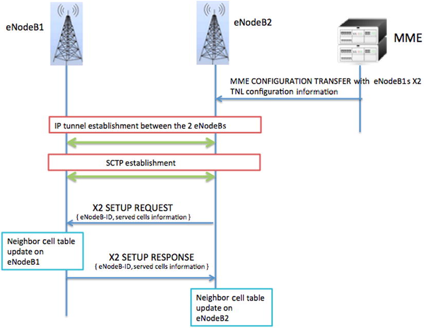
Figure 2-9. X2 setup and exchange of configurations between the two eNodeBs
Neighbor Relation Optimization
Broadly, there are two types of neighbor relations. First, there is a neighbor site relation, wherein there is a direct X2 connection existing between the two sites. In this case, the communication link between the two neighbors is known. Second, there is a neighbor cell relation, wherein the given two cells have a common or overlapping coverage area. UE always reposts a neighbor cell relation, but never a neighbor site relation, and only properly configured neighboring relations are relevant for handover performance figures. Figure 2-10 depicts these relations.

Figure 2-10. Neighbor cell and site relations
Referring to the example given in Figure 2-10:
- The eNodeB 1 has an X2 connection to the eNodeB 2 to neighbor site relation
- The eNodeB 2 parents three cells with PCIDs PCI 4, PCI 5, and PCI 6
- A neighbor cell relation exists only to the cell with PCID 6
When a new neighbor site relation is established, the configuration information of all parented cells is stored in the neighbor cell list. But only the identified and respectively measured neighbor cell is listed as a relation in the neighbor relation table (NRT) between one cell and a neighboring cell of this site.
During daily operation, a cell relation could fail to work properly for handovers (i.e., handover performance counters show higher failure rates than average). In this case, optimization algorithms can blacklist a relation.
Another possible optimization to the NRT is to mark the neighboring cells that are either under congestion or in temporary outage where handover is not allowed (shown by the field handover allowed in Figure 2-11). By doing this, the system information block (SIB) for the serving cell can be updated to avoid the cell information that is congested or blacklisted. The RRC connection setup and RRC connection reconfiguration messages sent by the serving cell to the UEs can be updated to remove measurement criteria for the cell. This information can also be used when UE reports measurement to the serving cell; if there are multiple reports from the UE, the serving cell can ignore the measurement report for the cell that is marked as handover not allowed and proceed with handover preparations for the other measured cells by the UE.

Figure 2-11. Neighbor site and cell list and neighbor relation table
The NRT can be further optimized to improve the KPIs for a particular neighbor by adding an X2 link if there are too many handovers performed between the two cells or eNodeBs and there is no existing X2AP link between the two. Considering that the X2AP links that can be maintained by an eNodeB are often limited, there needs to be some mechanism for the eNodeB to decide on maintaining an X2 link with one eNodeB over another. One way to achieve this is for the eNodeB to maintain a priority tag against each neighbor in the NRT and update it at a predetermined interval based on the number of handovers performed between the two eNodeBs and the percentage of handover failure for the pair and the operator to which the neighboring eNodeB belongs. With this combination, the eNodeB should be able to use the X2 links only between high-priority neighbors and release the X2 link for the lower-priority neighbor. A sample NRT is shown in Figure 2-11 with some useful information for each of the neighbors.
SON and Self-Optimization Motivation of Intercell Interference Coordination
The LTE systems operate mainly with a reuse 1 factor, as this helps maximize the capacity and bandwidth usage. However, this also means that there is a very high scope of interference for the UEs that are at the cell edge. Depending on the measured signal strength from the neighboring cell at the cell edge, the interference can lead to a high performance or throughput loss for the cell edge users. In turn, this will lead to a drop in spectral efficiency for the entire network. Intercell interference coordination (ICIC) solutions try to bring balance between the cell throughput and cell edge users’ data rate.
Principle of ICIC and Frequency Reuse
Frequency reuse is one of the best means to reduce intercell interference. The frequency reuse coefficient can be 1, 3 or 7. When the reuse coefficient equals 1 (i.e., adjacent cells are using the same frequency resource), at the cell edge, interference would be serious. A larger reuse coefficient can reduce intercell interference further, but care should be taken when doing this, as it will directly result in reduced spectral efficiency and cell throughput.
ICIC works on the principle wherein the frequency resource is divided into multiple frequency blocks (three blocks or seven blocks). Each cell will have a set of predefined physical resource blocks (PRBs) that are marked as cell center PRBs and another set of PRBs will be marked as cell edge PRBs.
Depending on the user location, a UE is either marked as a cell center UE or a cell edge UE, and the PRBs that are marked for cell center usage are provided to the cell center UEs. The PRBs that are marked for cell edge usage are provided to the cell edge UEs by the eNodeB scheduler.
Depending on the pattern of usage, care is taken to ensure that no two cells that are adjacent to each other will have the same set of PRBs marked as cell edge. Two UEs from neighboring cells (cell edge users) will not use the same set of PRBs, thereby reducing any interference to each other and improving the cell edge throughput. Figure 2-12 is an example of an ICIC deployment with a reuse coefficient pattern of 3.
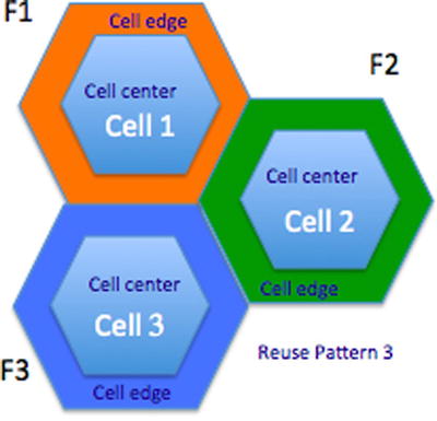
Figure 2-12. ICIC deployment with a reuse coefficient pattern of 3
ICIC may be of two types: static and dynamic.
- Static ICIC is a basic and simpler approach to implementing the ICIC feature. It is more suitable for cells that are predictable based on the type of traffic and the load distribution. In static ICIC, the parameters are configured during eNodeB commissioning itself. There are no reconfigurations and signaling with peers to negotiate on the resourcing pattern involved in static ICIC. Though it is a simpler approach, it is not necessarily efficient, as the planning does not always cover the different loading conditions and can result in performance degradation.
- Dynamic ICIC is a more complex approach based on the traffic conditions and cell loading. Dynamic ICIC is more suitable for cells where the cell loads a condition and the user distribution within the cell is not always predictable. Reconfigurations are typically triggered as part of dynamic ICIC to bring a balance between the cell edge user throughput experience vs. spectral efficiency. As part of dynamic ICIC, there are resource negotiations between the two eNodeBs via the X2 link as well. Though it is not as simple to implement the dynamic ICIC, it is more efficient and practical, as the cell sizes and the user distribution pattern in any network are not uniform.
Some of the key aspects that should be considered when designing and implementing ICIC with fractional frequency reuse mechanism are:
- Implementing fractional frequency reuse. In the downlink, the fractional frequency reuse (FFR) scheme can be based on a preferred list of red, blue, greens (RBGs; color scheme). For each sector, its edge band consists of a subset of PRBs listed earlier in the list, and its center band consists of the remaining PRBs in the list. The common control channels of a given sector are assigned edge PRBs to the maximum extent possible to avoid overlapping with edge PRBs of neighboring sectors. Further, it could be made flexible by allowing the operator to configure the number of PRBs that are reserved for cell edge and cell center.
- Cell edge UE identification. Considering the fact that the fractional frequency reuse design revolves around the PRB allocation for UEs ranged at different distances from the ENodeB, it becomes important that the UEs are classified as cell edge or cell center as accurately as possible for optimized results.
There can be different mechanisms used by different vendors to indentify the UE as a cell edge user. One of the most popular methods to determine or classify the UE as a cell edge user is based on the UE reported RSRP or RSRQ. Typically, there would be a configurable threshold value that can be set per the operator’s requirement. When the reported or average RSRQ or RSRP value from the UE goes below the threshold value, the UE can be classified as a cell edge UE. Further, the bandwidth allocation for cell edge users can be either static or dynamic.
In static resource allocation, the frequency band for the cell edge users and cell center users are statically configured. In dynamic resource allocation, for each subframe, the target allocation bandwidth is determined by resource usage in past subframes.
When the system is less loaded, all users will be scheduled within the edge band only when the system is overloaded beyond a particular threshold. Edge users will be scheduled in the edge band, and center users will be scheduled in the center band.
RACH Optimization
In LTE, a random access procedure can be performed by user equipment under the following conditions:
- IDLE user equipment performs an initial access procedure to move to the CONNECTED state.
- User equipment performs a handover to a target cell.
- When user equipment is in a CONNECTED state but out of time, synchronization occurs with the network, and it receives downlink data.
- When a UE is in a CONNECTED state but out of time, synchronization occurs with the network, and it attempts to transmit uplink data.
- When a UE performs reestablishment after it detects a radio link failure.
Need for RACH Optimization
In a homogenous network wherein the neighboring cells are using the same center frequency for uplink transmission, PRACH planning becomes very important and can very well be performed using self-optimization techniques.
User equipment that intends to move from an IDLE to a CONNECTED state to send or receive data will need to first perform a RANDOM ACCESS procedure.
The necessarily cell-specific RANDOM ACCESS procedural details are provided to the UE in systemInformationBlockType2 (SIB2). Each of these broadcasted SIB2 parameters can be fine tuned or optimized by the network in order to:
- Optimize the balance between the RANDOM ACCESS opportunities and UL data transfer. This is especially a concern in TDD modes of operation where there are not too many uplink opportunities for data transmissions, as well as RANDOM ACCESS procedures. During busy hours, when there are many users already connected to the cell and many more trying to connect to the cell by means of RANDOM ACCESS procedures, it becomes very important for the operator to be able to select the right base station setting for RANDOM ACCESS opportunities in order to balance the distribution of the uplink subframes between RANDOM ACCESS opportunities and user data transfer opportunity.
- Reduce interference during a RANDOM ACCESS procedure. In a homogeneous network, where there are multiple cells deployed, there is a huge probability of uplink interference that can result in performance drops for the entire network. Care should be taken to ensure that the neighboring cells that are operating at the same frequency avoid using the same root sequence number. Also it is very important to ensure that the PRACH opportunities between the two neighboring cells are different and do not have RACH opportunities at the same time and frequency.
- Reduce call setup and handover delays. This is extremely important in a deployment where there are users who are traveling at a higher speed.
The RACH optimization feature aims at automatically fine tuning the RACH parameters to enhance system performance. One of the targets listed in Table 2-1 should be used. Some of the performance targets that are configured by the operator as per the guidelines from 3GPP specs are outlined in the table.
Table 2-1. Performance Targets from 3GPP Specifications
Target Name |
Definition |
Legal Values |
|---|---|---|
Access probability (AP) |
The probability that the UE has for accessing the network after a certain number of random access attempts. |
Cumulative Distribution Function (CDF) of access attempts |
Access delay probability (ADP) |
The probability of the delay that an UE can experience while accessing the RACH. |
CDF of delays |
RachOptAccessDelayProbability |
This defines the list of ADPs that is acceptable. For a sampling period of time, each entry in the ADP list defines the maximum time delay before an UE can access the random access channel with a specific success percentage. This target is suitable for RACH Optimization (RO) |
ADPs are listed as a pair (a,b). An a in the list represents probability in percentages and a b represents the delay in ms. If ADPx’s a is larger than that of ADPy, then ADPx’s b also has to be larger than the b of ADPy. |
RachOptAccessProbability |
This defines the list of Access Probability (APn) that is acceptable. Each instance of APn of the list is the probability that the UE gets access on the RACH within n number of attempts over an unspecified sampling period. For a sampling period, each entry in the APn list defines the probability of an UE to be able to access the RACH within n attempts. This target is suitable for RO. |
APn’s are listed as a pair (a, n). An a in the list represents probability in percentages and n represents the number of attempts. If APx’s a is larger than that of APy, then APx’s n has to be also larger than n of APy. |
roSwitch |
Indicates if the RACH optimization feature is activated or deactivated. |
On, off |
The parameters presented in Table 2-2 are broadcasted by a base station under SIB2 that corresponds to the PRACH characteristics.
Table 2-2. PRACH Configuration Elements
-- ASN1START | ||
PRACH-ConfigSIB ::= rootSequenceIndex prach-ConfigInfo } |
SEQUENCE { INTEGER (0..837), PRACH-CinfigInfo |
|
PRACH-Config ::= rootSequenceIndex prach-ConfigInfo } |
SEQUENCE { INTEGER (0..837), PRACH-CinfigInfo |
OPTIONAL -- Need ON |
PRACH-ConfigInfo ::= prach-ConfigIndex highSpeedFlag zeroCorrelationZoneConfig prach-FreqOffset } |
SEQUENCE { INTEGER (0..63) BOOLEAN, INTEGER (0..15) INTEGER (0..94) |
|
Prach-ConfigIndex
The parameter Prach-ConfigIndex provides the information about random access opportunities that are available in a particular sector of the UE. There are 64 possible values that a Prach-ConfigIndex can assume, and each value provides information about the network the UE can use to attempt random access:
- Preamble format of the PRACH used
- Number of PRACH opportunities
- System frames during which the PRACH opportunities are configured
- Subframes where the PRACH opportunities are configured by the network
The preamble format and parameters are shown in Figure 2-13.

Figure 2-13. Preamble format and paramters used for PRACH
For an FDD deployment, the number of PRACH opportunities within a subframe cannot exceed 1. However, due to the shortage of uplink opportunities in the TDD network, there can be up to six PRACH opportunities. In order to reduce the call setup delays or handover delays, one of the parameters that can be optimized is the Prach-ConfigIndex, which can enable multiple PRACH opportunities for a UE wanting to establish connection.
Mobility Robustness Optimization
Mobility robustness optimization aims to improve system performance by optimizing the handover parameters. There are three popular reasons for handover failures for any LTE network: too early handover, too late handover, and handovers to a wrong cell. The mobility robustness optimization feature tries to optimize the cell offsets for two neighboring cells in order to reduce the failures that occur for these reasons. Optimization of these failures not only helps reduce the call drop ratio, but also significantly brings down the signaling load on a cell or eNodeB. Mobility robustness is part of the 3GPP’s SON use cases (TR 36.902 V9.0.0).
During deployment, the operator defines a default set of configuration for the mobility parameters based on the type of deployment (e.g., urban, dense urban, small office, rural). This set of parameters (default parameterization) is not always optimal and might not yield the desired KPIs upon deployment. Mobility robustness features aim to target these cells that are not optimally configured to continuously improve the mobility parameters by fine tuning them until a desired result is obtained, hence improving the overall mobility performance. Detection of poor mobility performance is based on the long-term evaluation of certain mobility counters and KPIs.
The operator can further specify how mobility robustness should be fine tuned by being able to configure the trigger conditions and exit criteria for these triggers. Let’s have a look at the types of handover failures, how they can be detected, and what actions can be taken for each of these failures.
Late Handovers
Late handovers often result in a radio link failure to the established connection even before a handover procedure is initiated on the source eNodeB side or the handover procedure is completed on the target eNodeB side. Often, in a late handover case, the UE tries to reestablish the radio links with the destination eNodeB upon radio link failure.
A popular means to reduce or have a check on the late handover failures is to detect such RRC reestablishment messages sent across from the UE to the target eNodeB and send them across an RLF indicator to the original source eNodeB. There the source eNodeB will recognize this as a late handover and can appropriately adjust the cell individual offset (CIO) for that particular neighbor so the percentage of late handovers is reduced for the cell pair. This mechanism is described in detail in Section 22.4.2 of TS 36.300-990. The RLF indicator message is described in Section 8.3.9 of TS 36.423-960.
For cases where the source and destination cell pairs belong to the same eNodeB, there will not be any X2 messaging to pass on the RLF indicator. Instead, the MRO corrective action will be taken care of by the eNodeB internally.
Figure 2-14 shows an example of how a late handover case is handled as part of the MRO solution.

Figure 2-14. How a late handover is handled as part of the MRO solution
Early Handovers
Early handovers often result in a radio link failure for a UE that has been handed over to a target cell after handover is complete. Often in an early handover case, the UE tries to reestablish the radio links with the previous source eNodeB upon radio link failure.
A very popular means to reduce or check on early handover failures is to detect such RRC reestablishment messages sent across from the UE to the source eNodeB and then send across an RLF indicator to the target eNodeB where the radio link failure occurred. The target eNodeB then recognizes the UE as the one that was originally handed over from the same eNodeB and sends across a handover report message to the original source eNodeB, thereby indicating this as an early handover case. In the source eNodeB, upon detecting this case as an early handover case, appropriate adjustments to the CIO for that particular neighbor can be carried out so the percentage of late handovers is reduced for the cell pair. This mechanism is described in detail in Section 22.4.2 of TS 36.300-990. RLF indicator message and handover report message are described in Sections 8.3.9 and 8.3.10 of TS 36.423-960.
For cases where the source as well as the destination cell pairs belong to the same eNodeB, there will not be any X2 messaging to pass on the RLF indicator or the handover report. Instead, the MRO corrective action will be taken care of by the eNodeB internally.
Figure 2-15 shows an example of how a too early handover case is handled as a part of the MRO solution.

Figure 2-15. Too early handover case is handled as a part of the MRO solution
Handover to Wrong Cell
Handovers often result in a radio link failure for a UE immediately after being handed over to a target cell, followed by the UE trying to reestablish the radio link connection with a cell that was not involved in the handover procedure. For example, after a successful handover from the cell belonging to eNodeB A to a cell belonging to eNodeB B, RLF happens, and the UE attempts connection reestablishment in the cell belonging to eNodeB C (as shown in Figure 2-16). In this case, eNodeB C sends an RLF indicator message to eNB B, followed by eNodeB B sending across a handover report message to eNodeB A indicating handover to the wrong cell. This mechanism is described in Section 22.4.2 of TS 36.300-990.

Figure 2-16. How handover to the wrong cell is handled
Note that the handover report message will be sent even if eNodeB B and eNodeB C are the same and RLF indication is internal to the eNodeB. Also, if handover fails during handover from a cell in eNodeB A and the UE attempts to reestablish the connection to a cell in eNodeB C, eNodeB C will then send an RLF indicator to eNodeB A.
In handover to a wrong cell, eNodeB A should note both eNodeB C and eNodeB B as handovers to the wrong cell CT (correct target) and handover to the wrong cell WT (wrong target) and adjust the corresponding cell individual offsets accordingly to reduce the rate of handover to wrong cell failure. Figure 2-16 shows an example case of how handover to the wrong cell case is handled as a part of the MRO solution.
Load Balancing
Clear load balancing strategy helps the multitechnology operator to optimize the use of their investments. Also, having a clear criteria for serving different types of traffic in certain network layer helps to ensure the capacity and service performance for mobile network subscribers. For these tasks, a centralized approach over the entire network area helps in minimizing the effort and time spent on load balancing.
Load balancing in LTE focuses mostly on air interface load balancing between different cells, between cells on the same of different frequency, and between different technology cells. Real-time load sharing is controlled with the handover triggering parameters and thresholds. The local optimization is based on real-time measurements.
There is also centralized support for load balancing in order to follow and ensure the adequate capacity in each network layer. Typically, the network management system collects the actual network statistics of load, handover, and cell performance and defines different criteria for these statistics based on the type of cell.
Typically, the central SON optimizer tool should be able to use the centralized information in other tools and analyze the load and handover performance against the actual parameters. The optimizer tool should be able to detect the cells continuously having high loads cells that are soon to reach the capacity limits and cells that experience the handover ping-pong effect and need optimization to improve the overall situation.
SON and Self-healing
Self-healing is one of the most important aspects of SON. There are various features that facilitate the self-healing aspect of SON, such as handover optimization, load balancing, cell outage detection and compensation, energy saving, among others. Each self-organization use case or feature involves fine tuning and optimizization of a set of parameters in a network element. The main goal for this parameter tuning is to enable self-configuration, self-optimization, and self-healing for the individual network elements or for the complete network as an entity. The main aim of self-healing is to detect a failure or outage and perform repair actions to recover the system from that outage or failure.
Let’s look at an example case of cell outage detection with compensation to further explain the SON self-healing mechanism.
Cell Outage Detection
Cell outage is detected by means of various alarms and alarm correlations. The outage can be from a service, process, or the complete cell itself. The network element should be designed to raise alarms or report counters or KPIs corresponding to these outages and pass it on toward the element manager system (EMS) for further actions. At the central SON level, outage KPIs are continuously monitored. If KPIs are below threshold or if the alarms for the network element exist for an extended period of time, the cell is then marked on the outage list by the central SON.
Cell Outage Compensation
As part of outage compensation, the central SON will need to detect the best set of cells that can compensate for the cell outage. The compensating set for an outage cell can be predetermined by the central SON, wherein for each cell, an outage compensation is calculated prior to and upon outage detection, and these compensation algorithms are then executed. The downside of this method in outage compensation is that the compensation calculation is static and does not consider the current load condition of the compensating cells. Also in the case of multiple outages within the network, the predetermined cell outage compensation algorithm will be suboptimal.
Another way to compensate for the outage cell is to dynamically (upon outage) determine the best cells that should be used for compensation. Some of the considerations for candidate cell selection can be:
- Proximity of the cell to the outage cell. Often the higher priority neighbors are selected as compensating cells as the amount of parameter tuning that will be required for these tier-1 neighbors will be comparitively lesser.
- Current load condition of the candidate cell. As a result of cell outage compensation, it is very likely that after the compensation procedure is performed, the candidate cells will have a larger coverage area with an increase in the number of users that are served by it. Also the incoming handover ratio can increase for the cell because of the compensation procedure. Care should be taken to ensure that the candidate cells are not already under high load condition with poor KPI performance.
- Type of the cell. Compensation algorithms will also consider the type of the candidate cell for any outage calculation (i.e., an indoor cell is not typically chosen as a candidate cell for compensation of an outdoor cell). Also, it is important that the candidate cell belongs to the same service provider so the impact to the revenue will be minimal.
The advantage of dynamically determining the candidate cells for compensation is that the estimation is more realistic and the risks are less as compared with that of static determination of the candidate cells. However, the time taken for the cell outage compensation will be much higher when performed dynamically.
As part of outage compensation, the parameters that are reconfigured on the candidate cells are typically cell mobility parameters, neighbor lists, cell transmit power, and antenna tilt. The tuning is performed in smaller steps and the KPIs are monitored for improvement. The action is stopped once the KPIs are in an acceptable range or the alarm for the outage is cleared.
Figure 2-17 presents a flowchart representing the cell outage compensation procedure for central SON.

Figure 2-17. Cell outage compensation procedure for central SON
Benefit of Cell Outage Compensation
There are three advantages to cell outage compensation procedures:
- Minimizes the damage and downtime until the faulty cell is repaired.
- Repair activity can be postponed or planned, as the impact will not be that high due to cell outage compensation. This will result in reduced maintenance costs (e.g., no permanent on-call service, smaller stocks of spare parts, combining of trips).
- Cell outage compensation is extremely useful and critical in places where the frequency of faults is higher.
Summary
This chapter provided a brief introduction to SON and its benefits and provided an overview of SON and its architecture, deployment aspects, and some of its major features. The following chapter talks in length about the deployment, business, and economic challenges that the fourth generation of mobile telecommunications technology is surrounded by.