
Chapter 18
Creating Spreadsheets with Numbers
IN THIS CHAPTER
![]() Getting familiar with and navigating Numbers
Getting familiar with and navigating Numbers
![]() Opening, saving, and formatting spreadsheets
Opening, saving, and formatting spreadsheets
![]() Selecting cells, entering data, and editing data
Selecting cells, entering data, and editing data
![]() Creating simple calculations
Creating simple calculations
![]() Adding charts to your spreadsheets
Adding charts to your spreadsheets
![]() Printing a Numbers spreadsheet
Printing a Numbers spreadsheet
Are you downright afraid of spreadsheets? Does the idea of building a budget with charts and all sorts of fancy graphics send you running for the safety of the hall closet? Well, good iMac owner, Apple has again taken something that everyone else considers to be super complex and turned it into something that normal human beings can use! (Much as Apple did with video editing and songwriting. Is there any type of software that Apple designers can’t make intuitive and easy to use?) And Numbers is a free download from the App Store, to boot!
In this chapter, I demonstrate how the Numbers spreadsheet program can help you organize data and analyze important financial decisions for home and business — everything from a household budget to your company’s sales statistics!
Before You Launch Numbers …
In case you’re unfamiliar with applications such as Numbers and Microsoft Excel — and the documents they create — let me provide you a little background information.
A spreadsheet organizes and calculates numbers by using a grid system of rows and columns. The intersection of each row and column is a cell, which can hold either text or numeric values. Cells can also hold calculations called formulas and functions, which are usually linked to the contents of surrounding cells.
Spreadsheets are wonderful tools for making decisions and comparisons because they let you plug in different numbers — such as interest rates or your monthly insurance premium — and instantly see the results. These are some of the spreadsheets that I use regularly:
- Car and mortgage loan comparisons
- A college planner
- My household budget (not that I pay any attention to it)
 Numbers can open, edit, and save documents created with Excel, but spreadsheets created with some advanced Excel features will not import properly, and Numbers will alert you if this happens. (The simpler the Excel spreadsheet, the more likely it is to open without significant errors.)
Creating a New Numbers Document
Like Pages (Apple’s desktop publishing application, which I cover in Chapter 17), Numbers ships with a selection of templates you can modify quickly to create a new spreadsheet. After a few modifications, you can easily use the Budget, Loan Comparison, and Mortgage templates to create your own spreadsheets.
To create a spreadsheet project file, follow these steps:
- Click the Launchpad icon on the Dock.
- Click the Numbers icon.
Click the New Document button in the bottom-left corner of the Open dialog that appears.
Numbers displays the Choose a Template window, shown in Figure 18-1. (To display the Choose a Template window and start a new Numbers project at any time, just choose File ⇒ New.)
In the list on the left, select the type of document you want to create.
The document thumbnails in the center are updated with templates that match your choice.
- Click the template that most closely matches your needs.
- Click the Choose button to open a new document that uses the template you selected.
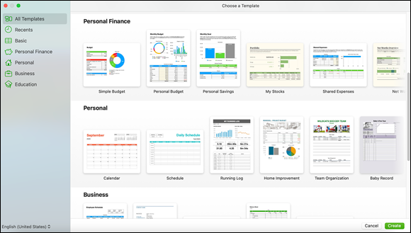
FIGURE 18-1: Hey, these templates aren’t frightening at all!
Opening an Existing Spreadsheet File
If you see an existing Numbers document in a Finder window (or you find it by using Spotlight), just double-click the Numbers document icon to open it. Numbers automatically loads and displays the spreadsheet.
It’s equally easy to open a Numbers document from within the program. Follow these steps:
- In Launchpad, click the Numbers icon to run the program.
Press ⌘ +O to display the Open dialog.
 As an iMac power user running macOS Monterey, you can save and load Numbers documents directly to and from your iCloud Drive. All three of Apple’s productivity applications — Pages, Numbers, and Keynote — feature an Open dialog that can display the contents of your iCloud Drive as well as those of your iMac’s internal drive. If the spreadsheet is stored in your iCloud Drive, click the Numbers item below the iCloud heading in the Sidebar on the left side of the dialog and then double-click the desired document thumbnail.
- If the document is stored in your iMac’s internal drive, on your network, or in one of your Favorites locations, click the desired drive or folder in the Sidebar on the left side of the dialog.
Drill down through folders and subfolders until you locate the desired Numbers document.
If you’re unsure where the document is, click the Search box at the top of the Open dialog and type a portion of the document name or even a word or two of text that it contains. Note that you can choose to search your drive, your iCloud Drive, or both.- Double-click the spreadsheet to load it.
If you want to open a spreadsheet you’ve been working on over the past few days, choose File ⇒ Open Recent to display Numbers documents that you’ve worked with recently.
Save Those Spreadsheets!
Thanks to the Auto-Save feature in Monterey, you need not fear losing a significant chunk of work because of a power failure or a coworker’s mistake. But if you’re not a huge fan of retyping data, period, you can save your spreadsheets manually after making a major change. Follow these steps to save your spreadsheet to your iCloud drive or your internal drive:
Press ⌘ +S.
If you’re saving a document that hasn’t yet been saved, the Save As sheet appears.
- Type a filename for your new spreadsheet.
Open the Where pop-up menu and choose a location in which to save the file.
Common locations are your iCloud Drive, Desktop, Documents folder, and Home folder.
If the location you want isn’t listed in the Where pop-up menu, click the down-arrow button next to the Save As text box to display the full Save As dialog. Click the desired drive in the Devices list on the left side of the dialog, and click folders and subfolders until you reach the desired location. Alternatively, type the folder name in the Spotlight Search box in the top-right corner, and double-click the desired folder in the list of matching names. (As a bonus, you can create a new folder in the full Save As dialog.)- Click Save.
After you save a Numbers document for the first time, you can create a version of that document by choosing File ⇒ Save. To revert to an older version of the current document, choose File ⇒ Revert To. You can revert to the last saved version or click Browse All Versions to look through multiple versions of the document and choose one of those versions to revert to.
Exploring the Numbers Window
Apple has done a great job of minimizing the complexity of the Numbers window. Figure 18-2 illustrates these major points of interest:
- Sheets tabs: Because a Numbers project can contain multiple spreadsheets, they’re displayed in the Sheets tabbed bar at the top of the window. To switch among spreadsheets in a project, click the desired tab.
- Sheet canvas: Numbers displays the rows and columns of your spreadsheet in this section of the window; you enter and edit cell values within the sheet canvas.
- Toolbar: The Numbers toolbar keeps the most common commands you’ll use within easy reach.
- Inspector: Located on the right side of the Numbers window, the Inspector displays editing controls for the object that’s currently selected, whether it’s text, a table, or a single cell. (If you enter an equal sign [=] in a cell to create a formula, the Inspector displays the Function list, where you can specify a calculation that Numbers should perform.)
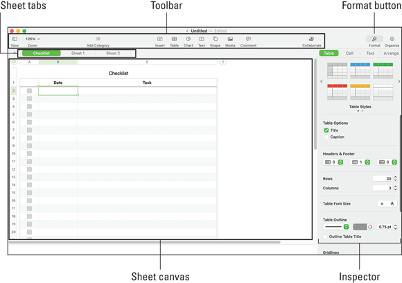
FIGURE 18-2: The Numbers window struts its stuff.
Navigating and Selecting Cells in a Spreadsheet
You can use the scroll bars to move around in your spreadsheet, but when you enter data into cells, moving your fingers from the keyboard is a hassle. Numbers has various handy shortcut keys you can employ, as shown in Table 18-1. After you commit these keys to memory, your productivity level will shoot straight to the top.
You can also use the mouse or trackpad to select cells in a spreadsheet:
- To select a single cell, click it.
- To select a range of adjacent cells, click a cell in any corner of the range you want and drag in the direction you want.
- To select a column of cells, click the alphabetic heading button at the top of the column.
- To select a row of cells, click the numeric heading button at the far-left end of the row.
TABLE 18-1 Movement Shortcut Keys in Numbers
Key or Key Combination | Where the Cursor Moves |
|---|---|
Left arrow (←) | One cell to the left |
Right arrow (→) | One cell to the right |
Up arrow (↑) | One cell up |
Down arrow (↓) | One cell down |
Home | To the beginning of the active worksheet |
End | To the end of the active worksheet |
Page Down | Down one screen |
Page Up | Up one screen |
Return | One cell down (also works within a selection) |
Tab | One cell to the right (also works within a selection) |
Shift+Enter | One cell up (also works within a selection) |
Shift+Tab | One cell to the left (also works within a selection) |
Entering and Editing Data in a Spreadsheet
After you navigate to the cell in which you want to enter data, you’re ready to type your data. Follow these steps to enter That Important Stuff:
Click the cell or press the spacebar.
A cursor appears, indicating that the cell is ready to hold any data you type.
Enter your data.
Spreadsheets can use both numbers and alphabetic characters within a cell; either type of information is considered to be data in the Spreadsheet World.- When you’re ready to move on, press Return (to save the data and move one cell down) or press Tab (to save the data and move one cell to the right).
Made a mistake? No big deal:
- To edit data: Click the cell that contains the data error (to select the cell); then click the cell again to display the insertion cursor. Drag the insertion cursor across the characters to highlight them, and type the replacement data.
To delete characters: Select the cell, highlight the characters, and press Delete.
You can quickly step backward through changes you’ve made and undo them by using the Undo command. Press Command+Z or choose Edit ⇒ Undo from the Numbers menu.
Selecting the Correct Number Format
After you enter your data (in a cell, row, or column), you may need to format it so that it appears correctly. Suppose that you want certain cells to display a specific type of number, such as a dollar amount, percentage, or date. Numbers gives you a healthy selection of number-formatting possibilities.
Characters and formatting rules — such as decimal places, commas, and dollar and percentage notation — are part of number formatting. If your spreadsheet contains units of currency, such as dollars, format it as such. Then all you need to do is type the numbers, and the currency formatting is applied automatically.
To specify a number format, follow these steps:
- Select the cells, rows, or columns you want to format.
- Click the Format toolbar button to display the Inspector.
- Click the Cell tab in the Inspector.
- From the Data Format pop-up menu, choose the type of formatting you want to apply, as shown in Figure 18-3.
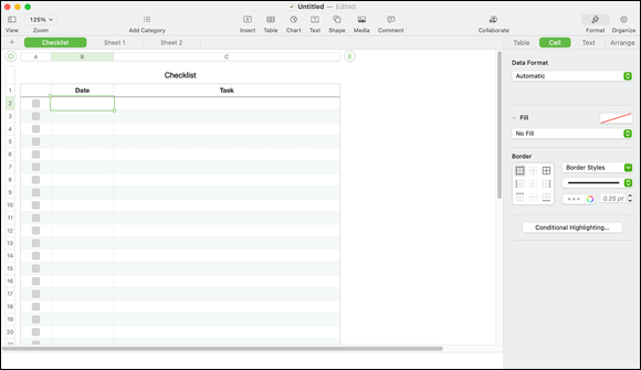
FIGURE 18-3: In the Inspector, you can format the data you’ve entered.
Aligning Cell Text Just So
You can also change the alignment of text in the selected cells, which can make a big difference in readability for titles and “crowded” data that’s packed into close columns. The default alignments are flush left for text and flush right for numeric data. Follow these steps:
Select the cells, rows, or columns you want to format.
See the earlier section “Navigating and Selecting Cells in a Spreadsheet” for tips on selecting stuff.
- Click the Format toolbar button.
- Click the Text tab of the Inspector to display the settings shown in Figure 18-4.
Click the corresponding Alignment button to choose the type of formatting you want to apply.
You can choose left, right, center, and justified text with the strip of buttons that appear under the Text Color section. Click the buttons in the second strip to specify the left and right indent levels for text. Text can be aligned at the top, center, or bottom of a cell using the third strip of buttons.
Do you need to set apart the contents of some cells? You might need to create text headings for some columns and rows or to highlight the totals in a spreadsheet, for example. To change such formatting, select the cells, rows, or columns you want to format; then click the Font Family, Font Size, or Font Color button on the Text tab.
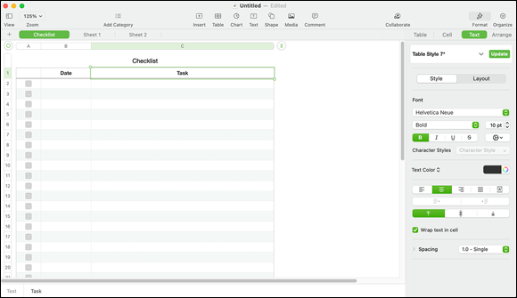
FIGURE 18-4: Set text alignment within a cell.
Formatting with Shading
Shading the contents of a cell, row, or column is helpful when your spreadsheet contains subtotals or logical divisions. Follow these steps to shade cells, rows, or columns:
- Select the cells, rows, or columns you want to format.
- Click the Format toolbar button.
- Click the Cell tab of the Inspector.
Click the triangle next to the Fill heading and choose a shading option from the Fill pop-up menu.
Figure 18-5 shows the controls for a gradient fill.
Click the color box to select a color for your shading.
Numbers displays a color picker wheel.
- Click at the desired spot within the wheel to select a color.
- After you achieve the effect you want, click the color box again to close the color picker.
You can also add a custom border to selected cells, rows, and columns from the Cell tab. Click the triangle next to the Border heading to select just the right border.
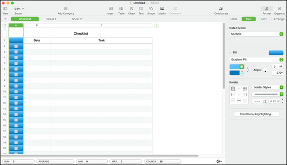
FIGURE 18-5: Adding shading and colors to cells, rows, and columns is easy in Numbers.
Inserting and Deleting Rows and Columns
What’s that? You forgot to add a row, and now you’re three pages into your data entry? No problem. You can easily add — or delete — rows and columns. First, select the row or column adjacent to where you want to insert (or delete) a row or column, and do one of the following:
- For a row: Right-click a row header and choose Add Row Above, Add Row Below, or Delete Row from the shortcut menu that appears.
- For a column: Right-click a column header and choose Add Column Before, Add Column After, or Delete Column from the shortcut menu that appears.
If you select multiple rows or columns, right-click and choose Add from the shortcut menu. Numbers inserts the same number of new rows or columns that you selected. You can also copy the contents of a row or column and paste them into any location in your spreadsheet.
You can also insert rows and columns via the Table menu at the top of the Numbers window.
The Formula Is Your Friend
It’s time to talk about formulas, which are equations that calculate values based on the contents of cells you specify in your spreadsheet. If you designate cell A1 (the cell in column A at row 1) to hold your yearly salary and cell B1 to hold the number 12, you can divide the contents of cell A1 by cell B1 (to calculate your monthly salary) by typing this formula in any other cell:
=A1/B1
Formulas in Numbers always start with an equal sign and may include one or more functions as well. A function is a preset mathematical, statistical, or engineering calculation that will be performed, such as figuring the sum or average of a series of cells.
“So what’s the big deal, Mark? Why not use a calculator?” Sure, you could. But maybe you want to calculate your weekly salary. Rather than grab a pencil and paper, you can simply change the contents of cell B1 to 52, and — boom! — the spreadsheet is updated to display your weekly salary.
That’s a simple example, of course, but it demonstrates the basics of using formulas (and the reason that spreadsheets are often used to predict trends and forecast budgets). It’s the what-if tool of choice for everyone who works with numeric data.
To add a simple formula within a spreadsheet, follow these steps:
- Select the cell that will hold the result of your calculation.
Type = (the equal sign).
The Formula box appears within the confines of the cell.
- Click the Format button on the Numbers toolbar to display the available functions in the Inspector, as shown in Figure 18-6.
Click the category of calculation you want from the left column of the Inspector.
Instead of scrolling through the entire function library, it’s easier to choose a category — such as Financial for your budget spreadsheet — to filter the selection. (Alternatively, you can click the Search box and type a function name or keyword.)
To display more information about a specific function, click it in the right column of the Inspector. In Figure 18-6, choosing the SUMfunction brings up a description at the bottom of the Inspector.After you select the perfect function in the right column, click the Insert Function button.
The function appears in the Formula box, along with any arguments it requires.
In case you're unfamiliar with the term argument, it refers to a value specified in a cell that a formula uses. The
SUMformula, for example, adds the contents of each cell you specify to produce a total; each of those cell values is an argument.Click an argument button in the formula and click the cell that contains the corresponding data.
Numbers automatically adds the cell you indicated to the formula.
- Repeat Step 6 for each argument in the formula.
- When you finish, click the Accept button — the green check mark — to add the formula to the cell.
That’s it! Your formula is ready to work behind the scenes, doing math for you so that the correct numbers appear in the cell you specified.

FIGURE 18-6: If you have to use formulas, at least Numbers can enter them for you.
Adding Visual Punch with a Chart
Sometimes you just have to see something to believe it, so it can help to use the data you’ve added to a spreadsheet to generate a professional-looking chart. After you’ve entered the data you want to chart, follow these steps:
Select the adjacent cells you want to chart by dragging.
To choose individual cells that aren’t adjacent, you can hold down the ⌘ key as you click.Click the Chart button on the Numbers toolbar.
The Chart button bears the symbol of a bar graph.
Numbers displays the thumbnail menu shown in Figure 18-7. Note that you can display different categories of charts by clicking one of the three tabs at the top (2D/3D/Interactive), and you can scroll the menu to reveal additional thumbnails by clicking the left- and right-arrow buttons.

FIGURE 18-7: Numbers displays the range of chart styles you can use.
Click the thumbnail for the chart type you want.
Numbers inserts the chart as an object within your spreadsheet so that you can move the chart. You can drag by using the handles that appear on the outside of the object box to resize your chart.
With your chart selected, click the Format toolbar button to display your old friend the Inspector, complete with the controls you can use to customize your chart’s appearance. You can change the colors and add (or remove) the title and legend, for example.- To change the default title, click the title box to select it; click it again to edit the text.
Printing Your Spreadsheet
You can easily send a Numbers spreadsheet to a USB or shared network printer. If you’d rather create an electronic copy of the document as an Adobe PDF file, you can click the PDF button that appears on the Numbers Print dialog; choose Save As PDF from the drop-down menu; and select a location where the file will be saved.
To print a Numbers spreadsheet on your default printer, follow these steps:
Choose File ⇒ Print from the Numbers menu bar.
Because a Numbers document can contain multiple spreadsheets, you can select a specific spreadsheet to print (by clicking it in the grid and then selecting the Print This Sheet radio button at the bottom-right corner of the window), or you can print all spreadsheets in the document (by selecting the Print All Sheets radio button in the same location).
Click the desired page orientation.
Spreadsheets with a large number of columns are often printed in landscape orientation to ensure that everything fits on the page. You can also scale the spreadsheet so that it automatically fits on the page by clicking the Fit button (next to the Content Scale slider).
Click Print at the bottom of the window.
Numbers displays the Print dialog. To display additional settings, click the Show Details button at the bottom of the sheet. (The PDF button appears in both views.)
- Click the Copies field and enter the number of copies you need.
- Select the pages to print:
- To print the entire spreadsheet, select All.
- To print a range of selected pages, select the From radio button and enter the starting and ending pages.
Click the Print button to send the document to your printer.
Click the Share menu item and choose the Send a Copy to share your spreadsheet masterpiece with others (as an actual copy of the document file). You can choose to send the copy via Mail, Messages, Notes, or AirDrop.