
2 Transact-SQL Data Type Nuances
“Don’t fix it if it ain’t broke” presupposes that you can’t improve something that works reasonably well already. If the world’s inventors had believed this, we’d still be driving Model A Fords and using outhouses.—H. W. Kenton
SQL Server includes a wide variety of built-in data types—more, in fact, than most other major DBMSs. It supports a wealth of character, numeric, datetime, BLOB, and miscellaneous data types. It offers narrow types for small data and open-ended ones for large data. SQL Server character strings can range up to 8000 bytes, while its BLOB types can store up to 2GB. Numeric values range from single-byte unsigned integers up to signed floating point values with a precision of 53 places. All except one of these data types (the cursor data type) are scalar types—they represent exactly one value at a time. There is an abundance of nuances, caveats, and pitfalls to watch out for as you use many of these types. This chapter will delve into a few of them.
SQL Server dates come in two varieties: datetime types and smalldatetime types. There is no separate time data type—dates and times are always stored together in SQL Server data. Datetime columns require eight bytes of storage and can store dates ranging from January 1, 1753, to December 31, 9999. Smalldatetime columns require four bytes and can handle dates from January 1, 1900, through June 6, 2079. Datetime columns store dates and times to the nearest three-hundredths of a second (3.33 milliseconds), while smalldatetime columns are limited to storing times to the nearest minute—they don’t store seconds or milliseconds at all.
If you wish to store a date without a time, simply omit the time portion of the column or variable—it will default to 00:00:00.000 (midnight). If you need a time without a date, omit the date portion—it will default to January 1, 1900. Dates default to January 1, 1900 because it’s SQL Server’s reference date—all SQL Server dates are stored as the number of days before or since January 1, 1900.
The date portion of a datetime variable occupies its first four bytes, and the time portion occupies the last four. The time portion of a datetime or smalldatetime column represents the number of milliseconds since midnight. That’s why it defaults to midnight if omitted.
One oddity regarding datetime columns of which you should be aware is the way in which milliseconds are stored. Since accuracy is limited to 3.33 milliseconds, milliseconds are always rounded to the nearest three-hundredths of a second. This means that the millisecond portion of a datetime column will always end in 0, 3, or 7. So, “19000101 12:00:00.564” is rounded to “19000101 12:00:00.563” and “19000101 12:00:00.565” is rounded to "19000101 12:00:00.567."
With the arrival of year 2000, it’s appropriate to discuss the impact the Y2K problem on SQL Server apps and some ways of handling it. A lot of hysteria seems to surround the whole Year 2000 issue—on the part of technical and nontechnical people alike—so it seems worthwhile to take a moment and address the way in which the Y2K problem affects SQL Server and applications based on it.
First, due to the fact that SQL Server sports a datetime data type, many of the problems plaguing older applications and DBMSs simply don’t apply here. Dates are stored as numeric quantities rather than character strings, so no assumptions need be made regarding the century, a given datetime variable, or column references.
Second, given that even a lowly smalldatetime can store dates up to 2079, there’s no capacity issue, either. Since four bytes are reserved for the date portion of a datetime column, a quantity of up to 2,147,483,647 days (including a sign bit) can be stored, even though there are only 3,012,153 days between January 1, 1753 and December 31, 9999.
Despite all this, there are still a number of subtle ways the Y2K and other date problems can affect SQL Server applications. Most of them have to do with assumptions about date formatting in T-SQL code. Consider the following:
SELECT CAST(’01-01-39’ AS datetime) AS DadsBirthDate
What date will be returned? Though it’s not obvious from the code, the date January 1, 2039 is the answer. Why? Because SQL Server has an internal century “window” that controls how two-digit years are interpreted. You can configure this with Enterprise Manager (right click your server, select Properties, then click Server Settings) or with sp_configure (via the two digit year cutoff setting). By default, two-digit years are interpreted by SQL Server as falling between 1950 and 2049. So, T-SQL code that uses the SELECT above and assumes it references 1939 may not work correctly. (Assuming 2039 for Dad’s birth year would mean that he hasn’t been born yet!)
The simplest answer, of course, is to use four-digit years. This disambiguates dates and removes the possibility that changing the two-digit year cutoff setting might break existing code. Note that I’m not recommending that you require four-digit dates in the user interfaces you build—I refer only to the T-SQL code you write. What you require of users is another matter.
Another subtle way that Y2K can affect SQL Server apps is through date-based identifiers. It’s not uncommon for older systems (and some newer ones) to use a year-in-century approach to number sequential items. For example, a purchase order system I rewrote in the eighties used the format YY-SequenceNumber to identify POs uniquely. These numbers were used as unique identifiers in a relational database system. Each time a new PO was added, a routine in the front-end application would search a table for the largest SequenceNumber and increment it by one. About five years before I became associated with the project, the company had merged with another company that had the same numbering scheme. In order to avoid duplicate keys, the programmer merging the two companies’ data simply added 10 to the year prefixes of the second company’s purchase orders. This, of course, amounted to installing a time bomb that would explode in ten years when the new keys generated for the first company’s data began to conflict with the second company’s original keys. Fortunately, we foresaw this situation and remedied it before it occurred. We remerged the two databases, this time adding to the SequenceNumber portion of the PO number, rather than its year prefix. We added a number to the second company’s sequence numbers that was sufficient to place them after all those of the first company, thus eliminating the possibility of future key conflicts.
This situation was not so much Y2K related as it was an imprudent use of date-based keys; however, consider the situation where the keys start with the year 1999. A two-digit scheme could not handle the rollover to 2000 because it could no longer retrieve the maximum sequence value from the database and increment it.
A common thread runs through all these scenarios: omitting the century portion of dates is problematic. Don’t do it unless you like problems.
SQL Server includes a number of functions to manipulate and work with datetime columns. These functions permit you to extract portions of dates, to add a quantity of date parts to an existing date, to retrieve the current date and time, and so on. Let’s explore a few of these by way of some interesting date problems.
Consider the classic problem of determining for company employees the hire date anniversaries that fall within the next thirty days. The problem is more subtle than it appears—there are a number of false solutions. For example, you might be tempted to do something like this:
SELECT fname, lname, hire_date
FROM EMPLOYEE
WHERE MONTH(hire_date)=MONTH(GETDATE())
But this fails to account for the possibility that a thirty-day time period may span two or even three months. Another false solution can be found in attempting to synthesize a date using the current year and the hire date month and day, like this:
SELECT fname, lname, hire_date
FROM EMPLOYEE
WHERE CAST(CAST(YEAR(GETDATE()) AS varchar(4))+
SUBSTRING(CONVERT(char(8), hire_date,112),5,4) AS datetime) BETWEEN GETDATE()
AND GETDATE()+30
This solution fails to allow for the possibility that the synthesized date might not be valid. How? If the employee was hired in a leap year and the current year isn’t also a leap year, you’ll have a problem if her hire date was February 29. A rare possibility, yes, but one a good solution should take into account.
The best solution doesn’t know or care about the exact date of the anniversary. It makes use of the SQL Server DATEDIFF() function to make the actual anniversary date itself irrelevant. DATEDIFF() returns the difference in time between two dates using the date or time unit you specify. The function takes three parameters: the date part or unit of time in which you want the difference returned (e.g., days, months, minutes, hours) and the two dates between which you wish to calculate the amount of elapsed time. You can supply any date part you want, including q or qq for calendar quarters, as well as h, mi, ss, and ms for time parts. Here’s the code:
SELECT fname, lname, hire_date
FROM EMPLOYEE
WHERE DATEDIFF(yy, hire_date,GETDATE()+30) > DATEDIFF(yy, hire_date,GETDATE())
This code basically says, “If the number of years between the hire date and today’s date plus thirty days exceeds the number of years between the hire date and today’s date, a hire date anniversary must have occurred within those thirty days, regardless of the actual date.”
Note the use of simple arithmetic to add days to a datetime variable (in this case, the return value of the GETDATE() function). You can add or subtract days from datetime and smalldatetime variables and fields via simple arithmetic. Also note the use of the GETDATE() function. This does what its name suggests—it returns the current date and time.
Similar to DATEDIFF(), DATEADD() adds a given number of units of time to a datetime variable or column. You can add (and subtract, using negative numbers) all the normal date components, as well as quarters and time portions. In the case of whole days, it’s syntactically more compact to use simple date arithmetic than to call DATEDIFF(), but the results are the same.
DATEPART() and the YEAR(), MONTH(), and DAY() functions extract portions of a given date. In addition to the date parts already mentioned, DATEPART() can return the day of the week, the week of the year, and the day of the year as integers.
Beyond being able to add or subtract a given number of days from date via simple arithmetic, you can also subtract one date from another to determine the number of days between them, but you must be careful. SQL Server will return the number of days between the two dates, but if either of them contains a time portion, the server will also be forced to include fractional days in its computation. Since we are converting the result to an integer (without the cast, subtracting one SQL Server date from another yields a third date—not terribly useful), a time portion of twelve hours or more will be considered a full day. This is somewhat counterintuitive. For example, consider this code:
SELECT CAST(GETDATE()-’19940101’ AS int)
If GETDATE() equals 1999-01-17 20:47:40, SQL Server returns:
1843
However, DATEDIFF(dd, GETDATE(),’19940101’) returns:
1842
Why the discrepancy? Because DATEDIFF() looks at whole days only, whereas SQL Server’s simple date arithmetic considers fractional days as well. The problem is more evident if we cast to a floating point value instead of an integer, like so:
SELECT CAST(GETDATE()-’19940101’ AS float)
1842.8664351851851
So, there are 1842.87 days between January 1, 1994 and January 17, 1999 20:47:40, or, rounded to the nearest integer, 1843.
To get the two methods to return the same result, we could adjust the first date’s time to something before noon, like so:
SELECT CAST(CAST(’1999-01-17 11:47:40’ AS datetime)- ’19940101’ AS int)
Although this would work, your users may not appreciate having their data changed to accommodate schlocky code. It would be kind of like performing heart surgery to fix a broken stethoscope. Far better simply to remove the time from the computation since we don’t care about it:
SELECT CAST(CAST(CONVERT(char(8),GETDATE(),112) AS datetime)-’19940101’ AS int)
This technique converts the date to an eight-byte character string and then back to a date again in order to remove its time portion. The time then defaults to ‘00:00:00.000’ for both dates, alleviating the possibility of a partial day skewing the results.
A common problem with dates is determining the gaps between them, especially when a table of dates or times is involved. Consider the following scenario: Per company policy, employees at a given factory must clock in and out each time they enter or leave the assembly line. The line supervisor wants to know how much time each of her employees spends away from the factory floor. Here’s a script that sets up their timecard records:
CREATE TABLE timeclock
(Employee varchar(30),
TimeIn smalldatetime,
TimeOut smalldatetime
)
INSERT timeclock VALUES(’Pythia’,’07:31:34’,’12:04:01’)
INSERT timeclock VALUES(’Pythia’,’12:45:10’,’17:32:49’)
INSERT timeclock VALUES(’Dionysus’,’9:31:29’,’10:46:55’)
INSERT timeclock VALUES(’Dionysus’,’10:59:32’,’11:39:12’)
INSERT timeclock VALUES(’Dionysus’,’13:05:16’,’14:07:41’)
INSERT timeclock VALUES(’Dionysus’,’14:11:49’,’14:57:02’)
INSERT timeclock VALUES(’Dionysus’,’15:04:12’,’15:08:38’)
INSERT timeclock VALUES(’Dionysus’,’15:10:31’,’16:13:58’)
INSERT timeclock VALUES(’Dionysus’,’16:18:24’,’16:58:01’)
Pythia seems to be a dutiful employee, while Dionysus appears to be playing hooky quite a bit. A query to determine the number of minutes each employee spends away on break might look something like this:
Obviously, there are too many breaks—even Dionysus couldn’t have had more breaks than work periods. The deceptive thing about this is that the first row looks correct—Pythia appears to have taken a forty-one minute lunch. But problems begin to arise as soon as there are more than two TimeIn/TimeOut pairs for a given employee. In addition to correctly computing the time between Dionysus’ work periods, the query computes the difference in minutes between clock-outs and clock-ins that don’t correspond to one another. What we should be doing instead is computing each break based on the most recent clock-out, like so:
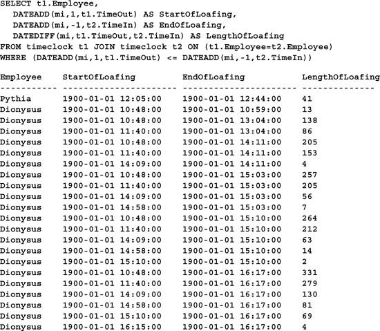
SELECT t1.Employee,
DATEADD(mi,1,t1.TimeOut) AS StartOfLoafing,
DATEADD(mi,-1,t2.TimeIn) AS EndOfLoafing,
DATEDIFF(mi,t1.TimeOut,t2.TimeIn) AS LengthOfLoafing
FROM timeclock T1 JOIN timeclock T2 ON (t1.Employee=t2.Employee)
WHERE (DATEADD(mi,1,t1.TimeOut)=
(SELECT MAX(DATEADD(mi,1,t3.TimeOut))
FROM timeclock T3
WHERE (t3.Employee=t1.Employee)
AND (DATEADD(mi,1,t3.TimeOut) <= DATEADD(mi,-1,t2.TimeIn))))
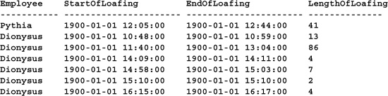
Notice the use of a correlated subquery to determine the most recent clock-out. It’s correlated in that it both restricts and is restricted by data in the outer query. As each row in T1 is iterated through, the value in its Employee column is supplied to the subquery as a parameter and the subquery is reexecuted. The row itself is then included or excluded from the result set based on whether its TimeOut value is greater than the one returned by the subquery. In this way, correlated subqueries and their hosts have a mutual dependence upon one another—a correlation between them.
The result set is about a third of the size of the one returned by the first query. Now Dionysus’ breaks seem a bit more believable, if not more reasonable.
You could easily extend this query to generate subtotals for each employee through Transact-SQL’s COMPUTE extension, like so:

Note the addition of an ORDER BY clause—a requirement of COMPUTE BY. COMPUTE allows us to generate rudimentary totals for a result set. COMPUTE BY is a COMPUTE variation that allows grouping columns to be specified. It’s quite flexible in that it can generate aggregates that are absent from the SELECT list and group on columns not present in the GROUP BY clause. Its one downside—and it’s a big one—is the generation of multiple results for a single query—one for each group and one for each set of group totals. Most front-end applications don’t know how to deal with COMPUTE totals. That’s why Microsoft has deprecated its use in recent years and recommends that you use the ROLLUP extension of the GROUP BY clause instead. Here’s the COMPUTE query rewritten to use ROLLUP:
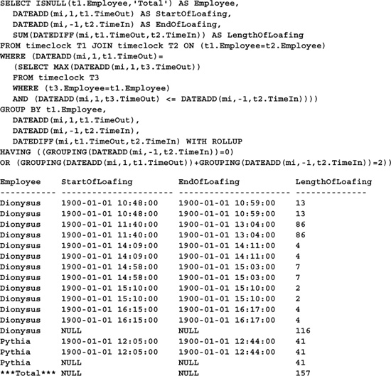
As you can see, the query is much longer. Improved runtime efficiency sometimes comes at the cost of syntactical compactness.
WITH ROLLUP causes extra rows to be added to the result set containing subtotals for each of the columns specified in the GROUP BY clause. Unlike COMPUTE, it returns only one result set. We’re not interested in all the totals generated, so we use a HAVING clause to eliminate all total rows except employee subtotals and the report grand total. The first set of NULL values in the result set corresponds to the employee subtotal for Dionysus. The second set marks Pythia’s subtotals. The third set denotes grand totals for the result set.
Note the use of the GROUPING() function to generate a custom string for the report totals line and to restrict the rows that appear in the result set. GROUPING() returns 1 when the specified column is being grouped within a particular result set row and 0 when it isn’t. Grouped columns are returned as NULL in the result set. If your data itself is free of NULLs, you can use ISNULL() in much the same way as GROUPING() since only grouped columns will be NULL.
Another common use of datetime fields is to build calendars and schedules. Consider the following problem: A library needs to compute the exact day a borrower must return a book in order to avoid a fine. Normally, this would be fourteen calendar days from the time the book was checked out, but since the library is closed on weekends and holidays, the problem is more complex than that. Let’s start by building a simple table listing the library’s holidays. A table with two columns, HolidayName and HolidayDate, would be sufficient. We’ll fill it with the name and date of each holiday the library is closed. Here’s some code to build the table:
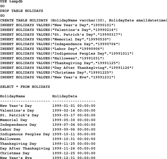
Next, we’ll build a table of check-out/check-in dates for the entire year. It will consist of two columns as well, CheckOutDate and DueDate. To build the table, we’ll start by populating CheckOutDate with every date in the year and DueDate with each date plus fourteen calendar days. Stored procedures—compiled SQL programs that resemble 3GL procedures or subroutines—work nicely for this because local variables and flow-control statements (e.g., looping constructs) are right at home in them. You can use local variables and control-flow statements outside stored procedures, but they can be a bit unwieldy and you lose much of the power of the language in doing so. Here’s a procedure that builds and populates the DUEDATES table:
USE tempdb
GO
DROP TABLE DUEDATES
GO
CREATE TABLE DUEDATES (CheckOutDate smalldatetime, DueDate smalldatetime)
GO
DROP PROC popduedates
GO
CREATE PROCEDURE popduedates AS
SET NOCOUNT ON
DECLARE @year integer, @insertday datetime
SELECT @year=YEAR(GETDATE()), @insertday=CAST(@year AS char(4))+’0101’
TRUNCATE TABLE DUEDATES -- In case ran more than once (run only from tempdb)
WHILE YEAR(@insertday)=@year BEGIN
-- Don’t insert weekend or holiday CheckOut dates -- library is closed
IF ((SELECT DATEPART(dw,@insertday)) NOT IN (1,7))
AND NOT EXISTS (SELECT * FROM HOLIDAYS WHERE HolidayDate=@insertday)
INSERT DUEDATES VALUES (@insertday, @insertday+14)
SET @insertday=@insertday+1
END
GO
EXEC popduedates
Now that we’ve constructed the table, we need to adjust each due date that falls on a holiday or weekend to the next valid date. The problem is greatly simplified by the fact that the table starts off with no weekend or holiday check-out dates. Since check-ins and check-outs are normally separated by fourteen calendar days, the only way to have a weekend due date occur once the table is set up initially is by changing a holiday due date to a weekend due date—that is, by introducing it ourselves.
One approach to solving the problem would be to execute three UPDATE statements: one to move due dates that fall on holidays to the next day, one to move Saturdays to Mondays, and one to move Sundays to Mondays. We would need to keep executing these three statements until they ceased to affect any rows. Here’s an example:
CREATE PROCEDURE fixduedates AS
SET NOCOUNT ON
DECLARE @keepgoing integer
SET @keepgoing=1
WHILE (@keepgoing<>0) BEGIN
UPDATE #DUEDATES SET DateDue=DateDue+1
WHERE DateDue IN (SELECT HolidayDate FROM HOLIDAYS)
SET @keepgoing=@@ROWCOUNT
UPDATE #DUEDATES SET DateDue=DateDue+2
WHERE DATEPART(dw,DateDue)=7
SET @keepgoing=@keepgoing+@@ROWCOUNT
UPDATE #DUEDATES SET DateDue=DateDue+1
WHERE DATEPART(dw,DateDue)=1
SET @keepgoing=@keepgoing+@@ROWCOUNT
END
This technique uses a join to HOLIDAYS to adjust holiday due dates and the DATEPART() function to adjust weekend due dates. Once the procedure executes, you’re left with a table of check-out dates and corresponding due dates. Notice the use of @@ROWCOUNT in the stored procedure to determine the number of rows affected by each UPDATE statement. This allows us to determine when to end the loop—when none of the three UPDATEs registers a hit against the table. The necessity of the @keepgoing variable illustrates the need in Transact-SQL for a DO...UNTIL or REPEAT...UNTIL looping construct. If the language supported a looping syntax that checked its control condition at the end of the loop rather than at the beginning, we might be able to eliminate @keepgoing.
Given enough thought, we can usually come up with a better solution to an iterative problem like this than the first one that comes to mind, and this one is no exception. Here’s a solution to the problem that uses just one UPDATE statement.
CREATE PROCEDURE fixduedates2 AS
SET NOCOUNT ON
SELECT ’Fixing DUEDATES’ -- Seed @@ROWCOUNT
WHILE (@@ROWCOUNT<>0) BEGIN
UPDATE DUEDATES
SET DueDate=DueDate+CASE WHEN DATEPART(dw,DueDate)=6 THEN 3 ELSE 1 END
WHERE DueDate IN (SELECT HolidayDate FROM HOLIDAYS)
END
This technique takes advantage of the fact that the table starts off with no weekend due dates and simply avoids creating any when it adjusts due dates that fall on holidays. It pulls this off via the CASE function. If the holiday due date we’re about to adjust is already on a Friday, we don’t simply add a single day to it and expect later UPDATE statements to adjust it further—we add enough days to move it to the following Monday. Of course, this doesn’t account for two holidays that occur back to back on a Thursday and Friday, so we’re forced to repeat the process.
The procedure uses an interesting technique of returning a message string to “seed” the @@ROWCOUNT automatic variable. In addition to notifying the user of what the procedure is up to, returning the string sets the initial value of @@ROWCOUNT to 1 (because it returns one “row”), permitting entrance into the loop. Once inside, the success or failure of the UPDATE statement sets @@ROWCOUNT. Taking this approach eliminates the need for a second counter variable like @@keepgoing. Again, an end-condition looping construct would be really handy here.
Just when we think we have the best solution possible, further reflection on a problem often reveals an even better way of doing things. Tuning SQL queries is an iterative process that requires lots of patience. You have to learn to balance the gains you achieve with the pain they cost. Trimming a couple of seconds from a query that runs once a day is probably not worth your time, but trimming a few from one that runs thousands of times may well be. Deciding what to tune, what not to, and how far to go is a skill that’s gradually honed over many years.
Here’s a refinement of the earlier techniques that eliminates the need for a loop altogether. It makes a couple of reasonable assumptions in order to pull this off. It assumes that no more than two holidays will occur on consecutive days (or that a single holiday will never span more than two days) and that no two holidays will be separated by less than three days. Here’s the code:
CREATE PROCEDURE fixduedates3 AS
SET NOCOUNT ON
UPDATE DUEDATES SET DueDate=DueDate+
CASE WHEN (DATEPART(dw,DueDate)=6) THEN 3
WHEN (DATEPART(dw,DueDate)=5) AND
EXISTS
(SELECT HolidayDate FROM HOLIDAYS WHERE HolidayDate=DueDate+1) THEN 4
ELSE 1
END
FROM HOLIDAYS WHERE DueDate = HolidayDate
This solution takes Thursday-Friday holidays into account via its CASE statement. If it encounters a due date that falls on a Thursday holiday, it checks to see whether the following Friday is also a holiday. If so, it adjusts the due date by enough days to move it to the following Monday. If not, it adjusts the due date by a single day just as it would a holiday falling on any other day of the week.
The procedure also eliminates the subquery used by the earlier techniques. Transact-SQL supports the FROM extension to the ANSI/ISO UPDATE statement, which allows one table to be updated based on data in another. Here, we establish a simple inner join between DUEDATES and HOLIDAYS in order to limit the rows updated to those with due dates found in HOLIDAYS.
SQL Server string variables and fields are of the basic garden-variety type. Variable-length and fixed-length types are supported, with each limited to a maximum of 8000 bytes. Like other types of variables, string variables are established via the DECLARE command:
DECLARE @Vocalist char(20)
DECLARE @Song varchar(30)
String variables are initialized to NULL when declared and can be assigned a value using either SET or SELECT, like so:
SET @Vocalist=’Paul Rodgers’
SELECT @Song=’All Right Now’
You can concatenate string fields and variables using the 1 operator, like this:
SELECT @Vocalist+’ sang the classic ’+@Song+’ for the band Free’
Whether you should choose to create character or variable character fields depends on your needs. If the data you’re storing is of a relatively fixed length and varies very little from row to row, fixed character fields make more sense. Each variable character field carries with it the overhead associated with storing a field’s length in addition to its data. If the length of the data it stores doesn’t vary much, a fixed-length character field will not only be more efficiently stored, it will also be faster to access. On the other hand, if the data length varies considerably from row to row, a variable-length field is more appropriate. Variable character fields can also be more efficient in terms of SQL syntax. Consider the previous example:
SELECT @Vocalist+’ sang the classic ’+@Song+’ for the band Free’
Because @Vocalist is a fixed character variable, the concatenation doesn’t work as we might expect. Unlike variable-length @Song, @Vocalist is right-padded with spaces to its maximum length, which produces this output:
Paul Rodgers sang the classic All Right Now for the band Free
Of course, we could use the RTRIM() function to remove those extra spaces, but it would be more efficient just to declare @Vocalist as a varchar in the first place.
One thing to watch out for with varchar concatenation is character movement. Concatenating two varchar strings can yield a third string where a key character (e.g., the last character or the first character of the second string) shifts within the new string due to blanks being trimmed. Here’s an example:
SELECT au_fname+’ ’+au_lname
FROM authors
(Results abridged)
--------------------------------------------------
Abraham Bennet
Reginald Blotchet-Halls
Cheryl Carson
Michel DeFrance
Innes del Castillo
Ann Dull
Marjorie Green
Morningstar Greene
Burt Gringlesby
Due to character movement and because at least one of the names contains multiple spaces, there’s no easy way to extract the authors’ first and last names once they’ve been combined in this way. Since au_fname is a 20-character field, the first character of au_lname is logical character 21 in the concatenated name. However, that character has moved due to au_lname’s concatenation with a varchar (nonpadded) string. It is now in a different position for each author, making extricating the original names next to impossible. This may not be an issue—it may be what you intend—but it’s something of which you should be aware.
By default, SQL Server doesn’t trim trailing blanks and zeros from varchar or varbinary values when they’re inserted into a table. This is in accordance with the ANSI SQL-92 standard. If you want to change this, use SET ANSI_PADDING (or SET ANSI_DEFAULTS). When ANSI_PADDING is OFF, field values are trimmed as they’re inserted. This can introduce some subtle problems. Here’s an example:
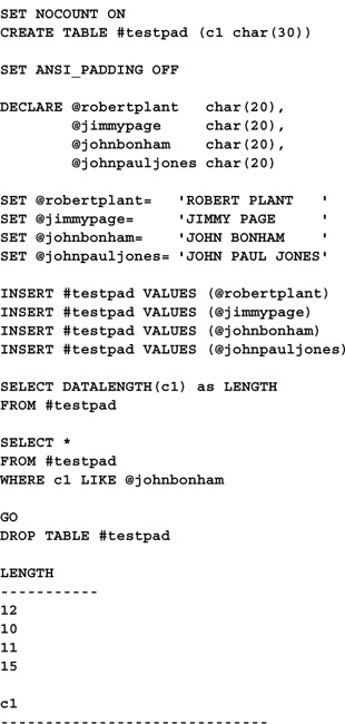
Because ANSI_PADDING has been turned OFF, no rows are returned by the second query even though we’re searching for a value we just inserted. Since ANSI_PADDING was disabled when @johnbonham was inserted, its trailing blanks were removed. That’s why the listed data lengths of the inserted values differ from row to row even though the ones we supplied were all the same length. When the second query attempts to locate a record using one of the inserted values, it fails because the value it’s using hasn’t been trimmed. The salient point here is that disabling ANSI_PADDING affects only the way values are stored—it doesn’t change the way that variables and constant values are handled. Since these are often used in comparison operations with stored values, a mismatch results—one value with trailing blanks and one without. That’s where subtle problems come in. As they say, the devil is in the details. Here’s what the result set would look like with ANSI_PADDING in effect:
LENGTH
-----------
15
15
15
15
c1
------------------------------
JOHN BONHAM
There are a number of SQL Server string functions. You can check the Books Online for specifics. I’ll take you through some of the more interesting ones.
The CHARINDEX() function returns the position of one string within another. Here’s an example:
SELECT CHARINDEX(’Now’,@Song)
You can optionally specify a starting position, like so:
SELECT CHARINDEX(’h’,’They call me the hunter’,17)
The SOUNDEX() function returns a string representing the sound of a character string. Like most soundex codes, Transact-SQL SOUNDEX() strings consist of a single character followed by three numeric digits. SOUNDEX() is most often used to alleviate the problems introduced by misspellings and typing mistakes in the database. Here’s an example of its use:
SELECT SOUNDEX(’Terry’), SOUNDEX(’Terri’)
Both of these expressions return a soundex of T600.
Transact-SQL’s implementation of SOUNDEX() isn’t terribly sophisticated, and it’s easy to fool it. Here’s an example:
SELECT SOUNDEX(’Rodgers’), SOUNDEX(’Rogers’)
You might think that these two surnames would have the same soundex, but that’s not the case. Usually, SOUNDEX() is used to implement limited fuzzy searches, to build mnemonic keys or codes, and the like. Because of its limitations, it’s pretty rare in real-life applications.
It’s easy enough to write a better phonetic matching routine than the one provided by SQL Server. Transact-SQL’s SOUNDEX() function is based on the original soundex algorithm patented by Margaret O’Dell and Robert Russell in 1918. To begin improving upon the stock function, let’s first rewrite it as a stored procedure. Here’s a stored procedure based on the O’Dell-Russell algorithm:
USE master
go
IF OBJECT_ID(’sp_soundex’) IS NOT NULL
DROP PROC sp_soundex
go
CREATE PROCEDURE sp_soundex @instring varchar(50), @soundex varchar(50)=NULL OUTPUT
/*
Object: sp_soundex
Description: Returns the soundex of a string
Usage: sp_soundex @instring=string to translate, @soundex OUTPUT=string in which to
return soundex
Returns: (None)
Created by: Ken Henderson. Email: [email protected]
Version: 7.0
Example: sp_soundex "Rodgers"
Created: 1998-05-15. Last changed: 1998-05-16.
Notes: Based on the soundex algorithm published by Robert Russell and Margaret O’Dell
in 1918.
Translation to Transact-SQL by Ken Henderson.
*/
AS
IF (@instring=’/?’) GOTO Help
DECLARE @workstr varchar(10)
SET @instring=UPPER(@instring)
SET @soundex=RIGHT(@instring,LEN(@instring)-1) -- Put all but the first char in a work
buffer (we always return the first char)
SET @workstr=’AEHIOUWY’ -- Remove these from the string
WHILE (@workstr<>’’) BEGIN
SET @soundex=REPLACE(@soundex,LEFT(@workstr,1),’’)
SET @workstr=RIGHT(@workstr,LEN(@workstr)-1)
END
/*
Translate characters to numbers per the following table:
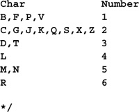
SET @workstr=’BFPV’
WHILE (@workstr<>’’) BEGIN
SET @soundex=REPLACE(@soundex,LEFT(@workstr,1),’1’)
SET @workstr=RIGHT(@workstr,LEN(@workstr)-1)
END
SET @workstr=’CGJKQSXZ’
WHILE (@workstr<>’’) BEGIN
SET @soundex=REPLACE(@soundex,LEFT(@workstr,1),’2’)
SET @workstr=RIGHT(@workstr,LEN(@workstr)-1)
END
SET @workstr=’DT’
WHILE (@workstr<>’’) BEGIN
SET @soundex=REPLACE(@soundex,LEFT(@workstr,1),’3’)
SET @workstr=RIGHT(@workstr,LEN(@workstr)-1)
END
SET @soundex=REPLACE(@soundex,’L’,’4’)
SET @workstr=’MN’
WHILE (@workstr<><>’’) BEGIN
SET @soundex=REPLACE(@soundex,LEFT(@workstr,1),’5’)
SET @workstr=RIGHT(@workstr,LEN(@workstr)-1)
END
SET @soundex=REPLACE(@soundex,’R’,’6’)
-- Now replace repeating digits (e.g., ’11’ or ’22’) with single digits
DECLARE @c int
SET @c=1
WHILE (@c<10) BEGIN
SET @soundex=REPLACE(@soundex,CONVERT(char(2),@c*11),CONVERT(char(1),@c)) -- Multiply
by 11 to produce repeating digits
SET @c=@c+1
END
SET @soundex=REPLACE(@soundex,’00’,’0’) -- Get rid of double zeros
SET @soundex=LEFT(@soundex,3)
WHILE (LEN(@soundex)<3) SET @soundex=@soundex+’0’ -- Pad with zero
SET @soundex=LEFT(@instring,1)+@soundex -- Prefix first char and return
RETURN 0
Help:
EXEC sp_usage @objectname=’sp_soundex’, @desc=’Returns the soundex of a string’,
@parameters=’@instring=string to translate, @soundex OUTPUT=string in which to
return soundex’,
@author=’Ken Henderson’, @email=’[email protected]’,
@datecreated=’19980515’, @datelastchanged=’19980516’,
@version=’7’, @revision=’0’,
@example=’sp_soundex "Rodgers"’
RETURN -1
Create this procedure, then test your new procedure using code like the following:
DECLARE @mysx varchar(4)
EXEC sp_soundex ’Rogers’,@mysx OUTPUT
SELECT @mysx,SOUNDEX(’Rogers’)
Your new procedure and the stock SOUNDEX() function should return the same code. Now let’s improve a bit on the original procedure by incorporating an optimization to the original algorithm introduced by Russell. Rather than merely removing the letters A, E, H, I, O, U, W, and Y, we’ll translate them to nines, remove repeating digits from the string, then remove the remaining nines from the string. Removing the nines after we’ve removed repeating digits reintroduces the possibility of repeating digits into the string and makes for finer granularity. This routine will perform better with a larger number of strings than the original routine. Here’s the revised routine:
USE master
go
IF OBJECT_ID(’sp_soundex_russell’) IS NOT NULL
DROP PROC sp_soundex_russell
go
CREATE PROCEDURE sp_soundex_russell @instring varchar(50), @soundex varchar(50)
=NULL OUTPUT
/*
Object: sp_soundex_russell
Description: Returns the soundex of a string (Russell optimization)
Usage: sp_soundex_russell @instring=string to translate, @soundex OUTPUT=string
in which to return soundex
Returns: (None)
Created by: Ken Henderson. Email: [email protected]
Version: 7.0
Example: sp_soundex_russell "Rodgers"
Created: 1998-05-15. Last changed: 1998-05-16.
Notes:
Based on the soundex algorithm published by Robert Russell and Margaret O’Dell
in 1918, extended to incorporate Russell’s optimizations for finer granularity.
*/
AS
IF (@instring=’/?’) GOTO Help
DECLARE @workstr varchar(10)
SET @instring=UPPER(@instring)
SET @soundex=RIGHT(@instring,LEN(@instring)-1) -- Put all but the first char in
a work buffer (we always return the first char)
/*
Translate characters to numbers per the following table:
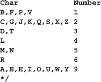
SET @workstr=’BFPV’
WHILE (@workstr<>’’) BEGIN
SET @soundex=REPLACE(@soundex,LEFT(@workstr,1),’1’)
SET @workstr=RIGHT(@workstr,LEN(@workstr)-1)
END
SET @workstr=’CGJKQSXZ’
WHILE (@workstr<>’’) BEGIN
SET @soundex=REPLACE(@soundex,LEFT(@workstr,1),’2’)
SET @workstr=RIGHT(@workstr,LEN(@workstr)-1)
END
SET @workstr=’DT’
WHILE (@workstr<>’’) BEGIN
SET @soundex=REPLACE(@soundex,LEFT(@workstr,1),’3’)
SET @workstr=RIGHT(@workstr,LEN(@workstr)-1)
END
SET @soundex=replace(@soundex,’L’,’4’)
SET @workstr=’MN’
WHILE (@workstr<>’’) BEGIN
SET @soundex=REPLACE(@soundex,LEFT(@workstr,1),’5’)
SET @workstr=RIGHT(@workstr,LEN(@workstr)-1)
END
set @soundex=replace(@soundex,’R’,’6’)
SET @workstr=’AEHIOUWY’
WHILE (@workstr<>") BEGIN
SET @soundex=REPLACE(@soundex,LEFT(@workstr,1),’9’)
SET @workstr=RIGHT(@workstr,LEN(@workstr)-1)
END
-- Now replace repeating digits (e.g., ’11’ or ’22’) with single digits
DECLARE @c int
SET @c=1
WHILE (@c<10) BEGIN
-- Multiply by 11 to produce repeating digits
SET @soundex=REPLACE(@soundex,CONVERT(char(2),@c*11),CONVERT(char(1),@c))
SET @c=@c+1
END
SET @soundex=REPLACE(@soundex,’00’,’0’) -- Get rid of double zeros
SET @soundex=REPLACE(@soundex,’9’,") -- Get rid of 9’s
SET @soundex=LEFT(@soundex,3)
WHILE (LEN(@soundex)<3) SET @soundex=@soundex+’0’ -- Pad with zero
SET @soundex=LEFT(@instring,1)+@soundex -- Prefix first char and return
RETURN 0
Help:
EXEC sp_usage @objectname=’sp_soundex_russell’, @desc=’Returns the soundex of a
string (Russell optimization)’,
@parameters=’@instring=string to translate, @soundex OUTPUT=string in which to
return soundex’,
@author=’Ken Henderson’, @email=’[email protected]’,
@datecreated=’19980515’, @datelastchanged=’19980516’,
@version=’7’, @revision=’0’,
@example=’sp_soundex_russell "Rodgers"’
RETURN -1
Like the original routine, this routine has a rather limited set of possible return codes—26 possible initial letters followed by three numerals, representing a maximum of 26 * 103, or 26,000 possible soundex codes. If we change the last three numerals to letters, we increase the number of possible return codes dramatically to 264 or 456,976. Here’s a soundex procedure that takes this approach:
USE master
GO
IF OBJECT_ID(’sp_soundex_alpha’) IS NOT NULL
DROP PROC sp_soundex_alpha
GO
CREATE PROCEDURE sp_soundex_alpha @instring varchar(50), @soundex varchar(50)=NULL
OUTPUT
/*
Object: sp_soundex_alpha
Description: Returns the soundex of a string
Usage: sp_soundex_alpha @instring=string to translate, @soundex OUTPUT=string in
which to return soundex
Returns: (None)
Created by: Ken Henderson. Email: [email protected]
Version: 7.0
Example: sp_soundex_alpha "Rodgers"
Created: 1998-05-15. Last changed: 1998-05-16.
Notes: Original source unknown.
Translation to Transact-SQL by Ken Henderson.
*/
AS
IF (@instring=’/?’) GOTO Help
DECLARE @workstr varchar(10)
SET @instring=UPPER(@instring)
SET @soundex=RIGHT(@instring,LEN(@instring)-1) -- Put all but the first char in
a work buffer (we always return the first char)
SET @workstr=’EIOUY’ -- Replace vowels with A
WHILE (@workstr<>’’) BEGIN
SET @soundex=REPLACE(@soundex,LEFT(@workstr,1),’A’)
SET @workstr=RIGHT(@workstr,LEN(@workstr)-1)
END
/*
Translate word prefixes using this table

-- Re-affix first char
SET @soundex=LEFT(@instring,1)+@soundex
IF (LEFT(@soundex,3)=’MAC’) SET @soundex=’MCC’+RIGHT(@soundex,LEN(@soundex)-3)
IF (LEFT(@soundex,2)=’KN’) SET @soundex=’NN’+RIGHT(@soundex,LEN(@soundex)-2)
IF (LEFT(@soundex,1)=’K’) SET @soundex=’C’+RIGHT(@soundex,LEN(@soundex)-1)
IF (LEFT(@soundex,2)=’PF’) SET @soundex=’FF’+RIGHT(@soundex,LEN(@soundex)-2)
IF (LEFT(@soundex,3)=’SCH’) SET @soundex=’SSS’+RIGHT(@soundex,LEN(@soundex)-3)
IF (LEFT(@soundex,2)=’PH’) SET @soundex=’FF’+RIGHT(@soundex,LEN(@soundex)-2)
-- Remove first char
SET @instring=@soundex
SET @soundex=RIGHT(@soundex,LEN(@soundex)-1)
/*
Translate phonetic prefixes (those following the first char) using this table:
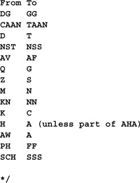
SET @soundex=REPLACE(@soundex,’DG’,’GG’)
SET @soundex=REPLACE(@soundex,’CAAN’,’TAAN’)
SET @soundex=REPLACE(@soundex,’D’,’T’)
SET @soundex=REPLACE(@soundex,’NST’,’NSS’)
SET @soundex=REPLACE(@soundex,’AV’,’AF’)
SET @soundex=REPLACE(@soundex,’Q’,’G’)
SET @soundex=REPLACE(@soundex,’Z’,’S’)
SET @soundex=REPLACE(@soundex,’M’,’N’)
SET @soundex=REPLACE(@soundex,’KN’,’NN’)
SET @soundex=REPLACE(@soundex,’K’,’C’)
-- Translate H to A unless it’s part of "AHA"
SET @soundex=REPLACE(@soundex,’AHA’,’~~~’)
SET @soundex=REPLACE(@soundex,’H’,’A’)
SET @soundex=REPLACE(@soundex,’~~~’,’AHA’)
SET @soundex=REPLACE(@soundex,’AW’,’A’)
SET @soundex=REPLACE(@soundex,’PH’,’FF’)
SET @soundex=REPLACE(@soundex,’SCH’,’SSS’)
-- Truncate ending A or S
IF (RIGHT(@soundex,1)=’A’ or RIGHT(@soundex,1)=’S’) SET
@soundex=LEFT(@soundex,LEN(@soundex)-1)
-- Translate ending "NT" to "TT"
IF (RIGHT(@soundex,2)=’NT’) SET @soundex=LEFT(@soundex,LEN(@soundex)-2)+’TT’
-- Remove all As
SET @soundex=REPLACE(@soundex,’A’,’’)
-- Re-affix first char
SET @soundex=LEFT(@instring,1)+@soundex
-- Remove repeating characters
DECLARE @c int
SET @c=65
WHILE (@c<91) BEGIN
WHILE (CHARINDEX(char(@c)+CHAR(@c),@soundex)<>0)
SET @soundex=REPLACE(@soundex,CHAR(@c)+CHAR(@c),CHAR(@c))
SET @c=@c+1
end
SET @soundex=LEFT(@soundex,4)
IF (LEN(@soundex)<4) SET @soundex=@soundex+SPACE(4-LEN(@soundex)) -- Pad with spaces
RETURN 0
Help:
EXEC sp_usage @objectname=’sp_soundex_alpha’, @desc=’Returns the soundex of a string’,
@parameters=’@instring=string to translate, @soundex OUTPUT=string in which to
return soundex’,
@author=’Ken Henderson’, @email=’[email protected]’,
@datecreated=’19980515’, @datelastchanged=’19980516’,
@version=’7’, @revision=’0’,
@example=’sp_soundex_alpha "Rodgers"’
RETURN -1
To see the advantages of this procedure over the more primitive implementation, try the following query:
DECLARE @mysx1 varchar(4), @mysx2 varchar(4)
EXEC sp_soundex_alpha ’Schuller’,@mysx1 OUTPUT
EXEC sp_soundex_alpha ’Shuller’,@mysx2 OUTPUT
SELECT @mysx1,@mysx2,SOUNDEX(’Schuller’),SOUNDEX(’Shuller’)
Thanks to its superior handling of common phonetic equivalents such as “SCH” and “SH,” sp_soundex_alpha correctly returns the same soundex code for Schuller and Shuller, while SOUNDEX() returns different codes for each spelling. Beyond the obvious use of identifying alternate spellings for the same name, the real reason we need a more complex routine like sp_soundex_alpha is to render more codes, not less of them. Consider the following test script:
DECLARE @mysx1 varchar(4), @mysx2 varchar(4)
EXEC sp_soundex_alpha ’Poknime’, @mysx1 OUTPUT
EXEC sp_soundex_alpha ’Poknimeister’,@mysx2 OUTPUT
SELECT @mysx1,@mysx2,soundex(’Poknime’),soundex(’Poknimeister’)
In this script, sp_soundex_alpha correctly distinguishes between the two names, while SOUNDEX() isn’t able to. Why? Because sp_soundex_alpha reduces the combination “KN” to “N,” thereby allowing it to consider the “S” at the end of “Poknimeister.” SOUNDEX(), by contrast, isn’t quite so capable. Since it leaves “KN” unaltered, the string it ends up translating for both names is PKNM, thus returning the same soundex code for each of them.
A companion to SOUNDEX(), DIFFERENCE() returns an integer indicating the difference between the soundex values of two character strings. The value returned ranges from 0 to 4, with 4 indicating that the strings are identical. So, using the earlier example:
SELECT DIFFERENCE(’Terry’, ’Terri’)
returns 4, while
SELECT DIFFERENCE(’Rodgers’, ’Rogers’)
returns 3.
Constructing a stored procedure to return the difference between two soundex codes is straightforward. Here’s an example:
USE master
GO
IF OBJECT_ID(’sp_soundex_difference’) IS NOT NULL
DROP PROC sp_soundex_difference
GO
CREATE PROCEDURE sp_soundex_difference @string1 varchar(50), @string2
varchar(50)=NULL, @difference int=NULL OUTPUT
/*
Object: sp_soundex_difference
Description: Returns the difference between the soundex codes of two strings
Usage: sp_soundex_difference @string1=first string to translate, @string2=second
string to translate, @difference OUTPUT=difference between the two as an integer
Returns: An integer representing the degree of similarity -- 4=identical,
0=completely different
Created by: Ken Henderson. Email: [email protected]
Version: 7.0
Example: sp_soundex_difference "Rodgers", "Rogers"
Created: 1998-05-15. Last changed: 1998-05-16.
*/
AS
IF (@string1=’/?’) GOTO Help
DECLARE @sx1 varchar(5), @sx2 varchar(5)
EXEC sp_soundex_alpha @string1, @sx1 OUTPUT
EXEC sp_soundex_alpha @string2, @sx2 OUTPUT
RETURN CASE
WHEN @sx1=@sx2 THEN 4
WHEN LEFT(@sx1,3)=LEFT(@sx2,3) THEN 3
WHEN LEFT(@sx1,2)=LEFT(@sx2,2) THEN 2
WHEN LEFT(@sx1,1)=LEFT(@sx2,1) THEN 1
ELSE 0
END
Help:
EXEC sp_usage @objectname=’sp_soundex_difference’, @desc=’Returns the difference
between the soundex codes of two strings’,
@parameters=’@string1=first string to translate, @string2=second string to translate,
@difference OUTPUT=difference between the two as an integer’,
@returns=’An integer representing the degree of similarity -- 4=identical, 0=completely
different’,
@author=’Ken Henderson’, @email=’[email protected]’,
@datecreated=’19980515’, @datelastchanged=’19980516’,
@version=’7’, @revision=’0’,
@example=’sp_soundex_difference "Rodgers", "Rogers"’
RETURN -1
Similar to a regular stored procedure, an extended procedure is accessed as though it was a compiled SQL program. In actuality, extended procedures aren’t written in Transact-SQL—they reside in DLLs (Dynamic Link Libraries) external to the server. They make use of the SQL Server ODS (Open Data Services) API using a language tool capable of producing DLLs such as C11 or Delphi.
As you might have guessed, the xp_sprintf extended stored procedure works similarly to the C sprintf() function. You can pass it a variable, a format string, and a list of arguments in order to construct a string variable. Currently, only string arguments are supported, so you can’t pass integers or other data types directly—but you can use them indirectly by converting them to strings first. Here’s an example illustrating the use of xp_sprintf:
DECLARE @Line varchar(80), @Title varchar(30), @Artist varchar(30)
SET @Title=’Butterflies and Zebras’
SET @Artist=’Jimi Hendrix’
EXEC xp_sprintf @Line output,’%s sang %s’,@Artist,@Title
SELECT @Line
Here’s an example showing how to cast other types of variables and fields to strings in order to use them as arguments to xp_sprintf:
DECLARE @TotalMsg varchar(80), @Items varchar(20)
SELECT @Items=CAST(count(*) as varchar(20)) FROM ITEMS
EXEC master..xp_sprintf @TotalMsg output,’There were %s items on file’,@Items
PRINT @TotalMsg
Xp_sscanf is the inverse of xp_sprintf. Rather than putting variables into a string, xp_sscanf extracts values from a string and places them into user variables, similar to the C sscanf() function. Here’s an example:
DECLARE @s1 varchar(20),@s2 varchar(20),@s3 varchar(20),@s4 varchar(20),
@s5 varchar(20),@s6 varchar(20),@s7 varchar(20),@s8 varchar(20),
@s9 varchar(20),@s10 varchar(20),@s11 varchar(20),@s12 varchar(20)
EXEC master..xp_sscanf
’He Meditated for a Moment, Then Kneeling Over and Across the Ogre , King Arthur
Looked Up and Proclaimed His Wish : Now, Miserable Beasts That Hack The Secret
of the Ancient Code And Run the Gauntlet, Today I Bid You Farewell’, ’He %stated
for a Moment, Then Kneeling %cver and A%cross the Og%s , King Arthur Looked %cp
and Proclaimed His %s : Now, %s Beasts That %s The Secret %s the %cncient %s And
%cun the Gauntlet, Today I Bid Your Farewell’, @s1 OUT, @s2 OUT,
@s3 OUT, @s4 OUT, @s5 OUT, @s6 OUT, @s7 OUT, @s8 OUT, @s9 OUT, @s10 OUT, @s11
OUT, @s12 OUT
SELECT @s1+@s2+@s3+@s4+’? ’+@s5+’ ’+@s6+’, ’+@s5+’ ’+@s7+’ ’+@s8+’ ’+@s9+
’ ’+@s10+’ ’+@s11+@s12
Using the %s and %c sscanf() format specifiers laid out in the second string, this example parses the first string argument for the specified character strings arguments. The %s specifier extracts a string, while %c maps to a single character. As each string or character is extracted, it’s placed in the output variable corresponding to it sequentially. A maximum of 50 output variables may be passed into xp_sscanf. You can run the query above (like the other queries in this chapter, it’s also on the accompanying CD) to see how xp_sscanf works.
If you’ve used C’s sscanf() function before, you’ll be disappointed by the lack of functionality in the Transact-SQL version. Many of the format parameters normally supported by sscanf()—including width specifiers—aren’t supported, nor are data types other than strings. Nevertheless, for certain types of parsing, xp_sscanf can be very handy.
Using the PATINDEX() function, you can search string fields and variables using wildcards. Here’s an example:
DECLARE @Song varchar(80)
SET @Song=’Being For The Benefit Of Mr. Kite!’
SELECT PATINDEX(’%Kit%’,@Song)
As used below, PATINDEX() works very similarly to the LIKE predicate of the WHERE clause. The primary difference is that PATINDEX() is more than a simple predicate—it returns the offset of the located pattern as well—LIKE doesn’t. To see how similar PATINDEX() and LIKE are, check out these examples:
SELECT * FROM authors WHERE PATINDEX(’Green%’,au_lname)<>0
could be rewritten as
SELECT * FROM authors WHERE au_lname LIKE ’Green%’
Similarly,
SELECT title FROM titles WHERE PATINDEX(’%database%’,notes)<>0
can be reworked to use LIKE instead:
SELECT title FROM titles WHERE notes LIKE ’%database%’
PATINDEX() really comes in handy when you need to filter rows not only by the presence of a mask but also by its position. Here’s an example:
SET NOCOUNT ON
CREATE TABLE #testblob (c1 text DEFAULT ’ ’)
INSERT #testblob VALUES (’Golf is a good walk spoiled’)
INSERT #testblob VALUES (’Now is the time for all good men’)
INSERT #testblob VALUES (’Good Golly, Miss Molly!’)
SELECT *
FROM #testblob
WHERE c1 LIKE ’%good%’
SELECT *
FROM #testblob
WHERE PATINDEX(’%good%’,c1)>15
GO
DROP TABLE #testblob
c1
--------------------------------------------------------------------------------
-Golf is a good walk spoiled
Now is the time for all good men
Good Golly, Miss Molly!
c1
--------------------------------------------------------------------------------
-Now is the time for all good men
Here, the first query returns all the rows in the table because LIKE can’t distinguish one occurrence of the pattern from another (of course, you could work around this by enclosing the column reference within SUBSTRING() to prevent hits within its first fifteen characters). PATINDEX(), by contrast, allows us to filter the result set based on the position of the pattern, not just its presence.
The Transact-SQL EXEC() function and the sp_executesql stored procedure allow you to execute a string variable as a SQL command. This powerful ability allows you to build and execute a query based on runtime conditions within a stored procedure or Transact-SQL batch. Here’s an example of a cross-tab query that’s constructed at runtime based on the rows in the pubs..authors table:
USE pubs
GO
IF OBJECT_ID(’author_crosstab’) IS NOT NULL
DROP PROC author_crosstab
GO
CREATE PROCEDURE author_crosstab
AS
SET NOCOUNT ON
DECLARE @execsql nvarchar(4000), @AuthorName varchar(80)
-- Initialize the create script string
SET @execsql=’CREATE TABLE FIautxtab (Title varchar(80)’
SELECT @execsql=@execsql+’,[’+au_fname+’ ’+au_lname+’] char(1) NULL DEFAULT ""’
FROM authors
EXEC(@execsql+’)’)
DECLARE InsertScript CURSOR FOR
SELECT execsql=’INSERT ##autxtab (Title,’+’[’+a.au_fname+’ ’+a.au_lname+’])
VALUES ("’+t.title+’", "X")’
FROM titles t JOIN titleauthor ta ON (t.title_id=ta.title_id)
JOIN authors a ON (ta.au_id=a.au_id)
ORDER BY t.title
OPEN InsertScript
FETCH InsertScript INTO @execsql
WHILE (@@FETCH_STATUS=0) BEGIN
EXEC sp_executesql @execsql
FETCH InsertScript INTO @execsql
END
CLOSE InsertScript
DEALLOCATE InsertScript
SELECT * FROM ##autxtab
DROP TABLE ##autxtab
GO
EXEC author_crosstab
GO
(Result set abridged)
Title Abraham Bennet Reginald Blotchet-H
--------------------------------------------------------------- -------------- -------------------
But Is It User Friendly?
Computer Phobic AND Non-Phobic Individuals: Behavior Variations
Computer Phobic AND Non-Phobic Individuals: Behavior Variations
Cooking with Computers: Surreptitious Balance Sheets
Cooking with Computers: Surreptitious Balance Sheets
Emotional Security: A New Algorithm
Fifty Years in Buckingham Palace Kitchens X
Is Anger the Enemy?
Is Anger the Enemy?
Life Without Fear
Net Etiquette
Onions, Leeks, and Garlic: Cooking Secrets of the Mediterranean
Prolonged Data Deprivation: Four Case Studies
Secrets of Silicon Valley
Secrets of Silicon Valley
Silicon Valley Gastronomic Treats
Straight Talk About Computers
Sushi, Anyone?
Sushi, Anyone?
Sushi, Anyone?
The Busy Executive’s Database Guide
The Busy Executive’s Database Guide X
The Gourmet Microwave
The Gourmet Microwave
You Can Combat Computer Stress!
The cross-tab that this query builds consists of one column for the book title and one for each author. An “X” denotes each title-author intersection. Since the author list could change from time to time, there’s no way to know in advance what columns the table will have. That’s why we have to use dynamic SQL to build it.
This code illustrates several interesting techniques. First, note the shortcut the code uses to build the first rendition of the @execsql string variable:
SET @execsql=’CREATE TABLE ##autxtab (Title varchar(80)’
SELECT @execsql=@execsql+’,[’+au_fname+’ ’+au_lname+’] char(1) NULL DEFAULT ""’
FROM authors
The cross-tab that’s returned by the query is first constructed in a temporary table. @execsql is used to build and populate that table. The code builds @execsql by initializing it to a stub CREATE TABLE command, then appending a new column definition to it for each row in authors. Building @execsql in this manner is quick and avoids the use of a cursor—a mechanism for processing tables a row at a time. Compared with set-oriented commands, cursors are relatively inefficient, and you should avoid them when possible (see Chapter 13, “Cursors,” for more information). When the SELECT completes its iteration through the authors table, @execsql looks like this:
CREATE TABLE ##autxtab (Title varchar(80),
[Abraham Bennet] char(1) NULL DEFAULT "",
[Reginald Blotchet-Halls] char(1) NULL DEFAULT "",
[Cheryl Carson] char(1) NULL DEFAULT "",
[Michel DeFrance] char(1) NULL DEFAULT "",
...
[Akiko Yokomoto] char(1) NULL DEFAULT ""
All that’s missing is a closing parenthesis, which is supplied when EXEC() is called to create the table:
EXEC(@execsql+’)’)
Either EXEC() or sp_executesql could have been called here to execute @execsql. Generally speaking, sp_executesql is faster and more feature laden than EXEC(). When you need to execute a dynamically generated SQL string multiple times in succession (with only query parameters changing between executions), sp_executesql should be your tool of choice. This is because it easily facilitates the reuse of the execution plan generated by the query optimizer the first time the query executes. It’s more efficient than EXEC() because the query string is built only once, and each parameter is specified in its native data format, not first converted to a string, as EXEC() requires.
Sp_executesql allows you to embed parameters within its query string using standard variable names as placeholders, like so:
sp_executesql N’SELECT * FROM authors WHERE au_lname LIKE @au_lname’,
N’@au_lname varchar(40)’,@au_lname=’Green%’
Here, @au_lname is a placeholder. Though the query may be executed several times in succession, the only thing that varies between executions is the value of @au_lname. This makes it highly likely that the query optimizer will be able to avoid recreating the execution plan with each query run.
Note the use of the “N” prefix to define the literal strings passed to the procedure as Unicode strings. Unicode is covered in more detail later in this chapter, but it’s important to note that sp_executesql requires Unicode strings to be passed into it. That’s why @execsql was defined using nvarchar.
In this particular case, EXEC() is a better choice than sp_executesql for two reasons: It’s not called within a loop or numerous times in succession, and it allows simple string concatenation within its parameter list; sp_executesql, like all stored procedures, doesn’t.
The second half of the procedure illustrates a more complex use of dynamic SQL. In order to mark each title-author intersection with an “X,” the query must dynamically build an INSERT statement for each title-author pair. The title becomes an inserted value, and the author becomes a column name, with “X” as its value.
Unlike the earlier example, sp_executesql is used to execute the dynamically generated INSERT statement because it’s called several times in succession and, thanks to the concatenation within the cursor definition, doesn’t need to concatenate any of its parameters.
Since sp_executesql allows parameters to be embedded in its query string, you may be wondering why we don’t use this facility to pass it the columns from authors. After all, they would seem to be fine examples of query parameters that vary between executions—why perform all the concatenation in the cursor? The reason for this is that sp_executesql limits the types of replaceable parameters it supports to true query parameters—you can’t replace portions of the query string indiscriminately. You can position replaceable parameters anywhere a regular variable could be placed if the query were run normally (outside sp_executesql), but you can’t replace keywords, object names, or column names with placeholders—sp_executesql won’t make the substitution when it executes the query.
One final point worth mentioning is the reason for the use of the global temporary table. A global temporary table is a transient table that’s prefixed with “##” instead of “#” and is visible to all connections, not just the one that created it. As with local temporary tables, it is dropped when no longer in use (when the last connection referencing it ends).
It’s necessary here because we use dynamic Transact-SQL to create the cross-tab table, and local temporary tables created dynamically are visible only to the EXEC() or sp_executesql that created them. In fact, they’re deleted as soon as the dynamic SQL that created them ends. So, we use a global temporary table instead, and it remains visible until explicitly dropped by the query or the connection closes.
The biggest disadvantage to using global temporary tables over local ones is the possibility of name collisions. Unlike their local brethren, global temporary table names aren’t unique across connections—that’s what makes them globally accessible. Regardless of how many connections reference it, ##autxtab refers to exactly the same object in tempdb. If a connection attempts to create a global temporary table that another connection has already built, the create will fail.
We accepted this limitation in order to be able to create the table dynamically, but there are a couple of other options. First, the body of the procedure could have been written and executed as one big dynamic query, making local tables created early in the query visible to the rest of it. Second, we could create the table itself in the main query, then use dynamic T-SQL to execute ALTER TABLE statements to add the columns for each author in piecemeal fashion. Here’s a variation on the earlier procedure that does just that:
CREATE PROCEDURE author_crosstab2
AS
SET NOCOUNT ON
DECLARE @execsql nvarchar(4000), @AuthorName varchar(80)
CREATE TABLE #autxtab (Title varchar(80))
DECLARE AlterScript CURSOR FOR
SELECT ’ALTER TABLE #autxtab ADD [’+au_fname+’ ’+au_lname+’] char(1) NULL DEFAULT ""’
FROM authors
FOR READ ONLY
OPEN AlterScript
FETCH AlterScript INTO @execsql
WHILE (@@FETCH_STATUS=0) BEGIN
EXEC sp_executesql @execsql
FETCH AlterScript INTO @execsql
END
CLOSE AlterScript
DEALLOCATE AlterScript
DECLARE InsertScript CURSOR FOR
SELECT execsql=’INSERT #autxtab (Title,’+’[’+a.au_fname+’ ’+a.au_lname+’]) VALUES
("’+t.title+’", "X")’
FROM titles t JOIN titleauthor ta ON (t.title_id=ta.title_id)
JOIN authors a ON (ta.au_id=a.au_id)
ORDER BY t.title
OPEN InsertScript
FETCH InsertScript INTO @execsql
WHILE (@@FETCH_STATUS=0) BEGIN
EXEC sp_executesql @execsql
FETCH InsertScript INTO @execsql
END
CLOSE InsertScript
DEALLOCATE InsertScript
SELECT * FROM #autxtab
DROP TABLE #autxtab
Note the use of the AlterScript cursor to supply sp_executesql with ALTER TABLE queries. Since the table itself is created in the main query and since the temporary objects created in a query are visible to its dynamic queries, we’re able to get by with a local temporary table and eliminate the possibility of name collisions. Though this solution requires more code than the initial one, it’s also much safer.
Note that this object visibility doesn’t carry over to local variables. Variables defined by the calling routine are not visible to EXEC() or sp_executesql. Also, variables defined within an EXEC() or call to sp_executesql go out of scope when they return to the caller. Basically, the only way to pass variables between them is via sp_executesql’s parameter list or via concatenation within the EXEC call.
In the past, character string data was limited to characters from sets of 256 characters. Each character was composed of a single byte and a byte can store just 256 (28) different characters. Prior to the adoption of the Unicode standard, all character sets were composed of single-byte characters.
Unicode expands the number of possible characters to 216, or 65,536, by using two bytes instead of one. This increased capacity facilitates the inclusion of the alphabets and symbols found in most of the world’s languages, including all of those from the single-byte character sets used previously.
Transact-SQL’s regular string types (char, varchar, and text) are constructed of characters from a particular single-byte character set. This character set is selected during installation and can’t be changed afterward without recreating databases and reloading data. Unicode strings, by contrast, can store any character defined by the Unicode standard. Since Unicode strings take twice as much storage space as regular strings, they can be only half as long (4000 characters).
SQL Server defines special Unicode-specific data types for storing Unicode strings: nchar, nvarchar, and ntext. You can use these data types for columns that need to store characters from multiple character sets. As with regular character string fields, you should use nvarchar when a column’s data varies in length from row to row and nchar when it doesn’t. Use ntext when you need to store more than 4000 characters.
SQL Server’s Unicode string types are based on SQL-92’s National Character data types. As with SQL-92, Transact-SQL uses the prefix character N to distinguish Unicode data types and values, like so:
SELECT DATALENGTH(N’The Firm’)
-----------
16
This query returns “16” because the uppercase N makes ‘The Firm’ a Unicode string.
Transact-SQL supports four general classes of numeric data types: float and real, numeric and decimal, money and smallmoney, and the integer types (int, smallint, and tinyint). Float and real are floating point types—as such, they’re approximate, not exact types—and some values within their ranges (−1.79E + 308 to 1.79E + 308 and −3.40E + 38 to 3.40E + 38, respectively) can’t be represented precisely. Numeric and decimal are fixed-point numeric types with a user-specified, fixed precision and scale and a range of −1038 −1 to + 1038 −1. Money and smallmoney represent monetary quantities and can range from −263 to +263 −1 and −231 to +231 −1 with a scale of four (−-214,748.3648 to +214,748.3647), respectively.
Integer types represent whole numbers. The int data type requires four bytes of storage and can represent integers between −231 and +2231 −1. Smallint requires two bytes and can represent integers between −215 and +215 −1. Tinyint uses just one byte and stores integers between 0 and 255.
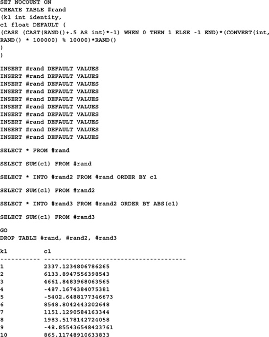
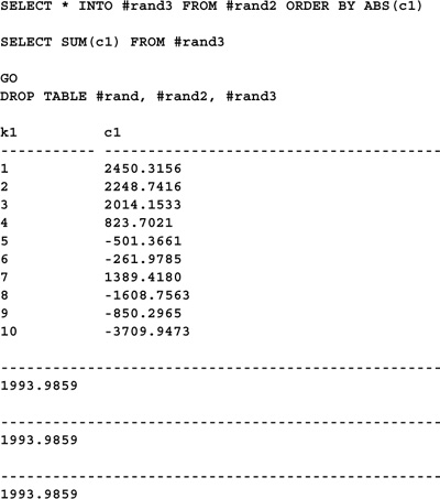
The first thing you discover when doing any real floating point work with SQL Server is that Transact-SQL does not correct for floating point rounding errors. This allows the same numeric problem, stated in different ways, to return different results—heresy in the world of mathematics. Languages that don’t properly handle floating point rounding errors are particularly susceptible to errors due to differences in the ordering of terms. Here’s an example that generates a random list of floating point numbers, then arranges them in various orders and totals them:
---------------------------------------------------
19742.763546549555
---------------------------------------------------
19742.763546549551
---------------------------------------------------
19742.763546549551
Since the numbers being totaled are the same in all three cases, the results should be the same, but they aren’t. Increasing SQL Server’s floating point precision (via the /p server command line option) helps but doesn’t solve the problem—floating point rounding errors aren’t handled properly, regardless of the precision of the float. This causes grave problems for applications that depend on floating point accuracy and is the main reason you’ll often see the complex floating point computations in SQL Server applications residing in 3GL routines.
The one foolproof answer here is to use fixed-point rather than floating point types. The decimal and numeric data types do not suffer from floating point rounding errors because they aren’t floating point types. As such, they also can’t use the processor’s FPU, so computations will probably be slower than with real floating point types. This slowness may be compensated for in other areas, so this is not as bad as it may seem. The moral of the story is this: SQL Server doesn’t correct floating point errors, so be careful if you decide to use the float or real data types.
Here’s the query rewritten to use a fixed-point data type with a precision of 10 and a scale of 4:

Prior to release 7.0 of SQL Server, dividing a numeric quantity by zero returned a NULL result. By default, that’s no longer the case. Dividing a number by zero now results in a divide by zero exception:
SELECT 1/0
Server: Msg 8134, Level 16, State 1, Line 1
Divide by zero error encountered.
You can disable this behavior via the ANSI_WARNINGS and ARITHIGNORE session settings. By default, ANSI warnings are enabled when you connect to the server using ODBC or OLEDB, and ARITHIGNORE is disabled. Here’s the query modified to return NULL when a divide by zero occurs:
SET ANSI_WARNINGS OFF
SET ARITHIGNORE ON
SELECT 1/0
---------------------------------------------------
NULL
(If you’re executing this query from Query Analyzer, you’ll need to disable ANSI warnings in the Current Connection Options dialog in order for this to work.)
There’s an inconsistency between the monetary types—money and smallmoney—and the other numeric data types. All numerics except for money and smallmoney implicitly convert from character strings during INSERTs and UPDATEs. Money and smallmoney, for some reason, have problems with this. For example, the following query generates an error message:
CREATE TABLE #test (c1 money)
-- Don’t do this -- bad SQL
INSERT #test VALUES(’1232’)
SELECT *
FROM #test
GO
DROP TABLE #test
You can change c1’s data type to any other numeric type—from tinyint to float—and the query will execute as you expect. The monetary types, for some reason, are more finicky. They require an explicit cast, like so:
CREATE TABLE #test (c1 money)
INSERT #test SELECT CAST(’1232’ AS money)
SELECT *
FROM #test
GO
DROP TABLE #test
c1
---------------------
1232.0000
In addition to using CAST() and CONVERT() to format numeric data types as strings, you can use the STR() function. STR() is better than the generic CAST() and CONVERT() because it provides for right justification and allows the number of decimal places to be specified. Here are some examples:
SELECT STR(123,10) AS Str,
CAST(123 AS char(10)) AS Cast
Str Cast
--- -----------------
123 123
SELECT STR(PI(),7,4) AS Str,
CAST(PI() AS char(7)) AS Cast
Str Cast
------ --------------
3.1416 3.14159
SQL Server provides support for BLOB (binary large object) fields via its image and text (and ntext) data types. These data types permit the storage and retrieval of fields up to 2GB in size. With the advent of 8000-byte character strings, much of the need for these has gone away, but with more and more nontraditional data types being stored in SQL Server databases everyday, BLOB fields are definitely here to stay.
As implemented by SQL Server, BLOB fields are somewhat ponderous, and you should think twice before including one in a table definition. BLOB fields are stored in a separate page chain from the row in which they reside. All that’s stored in the BLOB column itself is a sixteen-byte pointer to the first page of the column’s page chain. BLOBs aren’t stored like other data types, and you can’t treat them as though they were. You can’t, for example, declare text or image local variables. Attempting to do so generates a syntax error. You can pass a text or image value as a parameter to a stored procedure, which you can then use in a DML statement, but you can’t reassign the variable or do much else with it. Here’s a procedure that illustrates:
CREATE PROCEDURE inserttext @instext text
AS
SET NOCOUNT ON
SELECT @instext AS ’Inserting’
CREATE TABLE #testnotes (k1 int identity, notes text)
INSERT #testnotes (notes) VALUES (@instext)
SELECT DATALENGTH(notes), *
FROM #testnotes
DROP TABLE #testnotes
GO
EXEC inserttext ’TEST’
Inserting
---------------------------------------------------
TEST
k1 notes
---------- ---------- ----------------------------------------------------------
4 1 TEST
Here, @instext is a text parameter that the stored procedure inserts into the text column notes. Since you can’t define local text variables, @instext can’t be assigned to another text variable (though it can be assigned to a regular char or varchar variable) and can’t have a different value assigned to it. For the most part, it’s limited to being used in place of a text value in a DML (Data Management Language) command.
You also can’t refer to BLOB columns in the WHERE clause using the equal sign—the LIKE predicate, PATINDEX(), or DATALENGTH() is required instead. Here’s an example:
CREATE TABLE #testnotes (k1 int identity, notes text)
INSERT #testnotes (notes) VALUES (’test’)
GO
-- Don’t run this -- doesn’t work
SELECT *
FROM #testnotes
WHERE notes=’test’
GO
DROP TABLE #testnotes
GO
Even though the INSERT statement has just supplied the ‘test’ value, the SELECT can’t query for it using the traditional means of doing so. You have to do something like this instead:
SELECT *
FROM #testnotes
WHERE notes LIKE ’test’
The normal rules governing data types and column access simply don’t apply with BLOB columns, and you should bear that in mind if you elect to make use of them.
Unlike smaller BLOBs, it’s not practical to return large BLOB data via a simple SELECT statement. Though you can use SET TEXTSIZE to control the amount of text returned by a SELECT, your front end may not be able to deal with large amounts of BLOB data properly. Moreover, since you can’t declare local text or image variables, you can’t use SELECT to assign a large BLOB to a variable for further parsing. Instead, you should use the READTEXT command to access it in pieces. READTEXT works with image as well as text columns. It takes four parameters: the column to read, a valid pointer to its underlying text, the offset at which to begin reading, and the size of the chunk to read. Use the TEXTPTR() function to retrieve a pointer to a BLOB column’s underlying data. This pointer is a binary(16) value that references the first page of the BLOB data. You can check its validity via the TEXTVALID() function. Here’s an example illustrating the use of TEXTPTR() and READTEXT:
DECLARE @textptr binary(16)
BEGIN TRAN
SELECT @textptr=TEXTPTR(pr_info)
FROM pub_info (HOLDLOCK)
WHERE pub_id=’1389’
READTEXT pub_info.pr_info @textptr 29 20
COMMIT TRAN
pr_info
--------------------------------------------------------------------------------
Algodata Infosystems
Notice the use of a transaction and the HOLDLOCK keyword to ensure the veracity of the text pointer from the time it’s first retrieved through its use by READTEXT. Since other users could modify the BLOB column while we’re accessing it, the pointer returned by TEXTPTR() could become invalid between its initial read and the call to READTEXT. We use a transaction to ensure that this doesn’t happen. People tend to think of transactions as being limited to data modification management, but, as you can see, they’re also useful for ensuring read repeatability.
Rather than specifying a fixed offset and read length, it’s more common to use PATINDEX() to locate a substring within a BLOB field and extricate it, like so:
DECLARE @textptr binary(16), @patindex int, @patlength int
BEGIN TRAN
SELECT @textptr=TEXTPTR(pr_info), @patindex=PATINDEX(’%Algodata
Infosystems%’,pr_info)-1,
@patlength=DATALENGTH(’Algodata Infosystems’)
FROM pub_info (HOLDLOCK)
WHERE PATINDEX(’%Algodata Infosystems%’,pr_info)<>0
READTEXT pub_info.pr_info @textptr @patindex @patlength
COMMIT TRAN
pr_info
--------------------------------------------------------------------------------
Algodata Infosystems
Note the use of PATINDEX() to both qualify the query and set the @patindex variable. The query must subtract one from the return value of PATINDEX() because PATINDEX() is one-based, while READTEXT is zero-based. As mentioned earlier, PATINDEX() works similarly to LIKE except that it can also return the offset of the located pattern or string.
Handling larger segments requires looping through the BLOB with READTEXT, reading it a chunk at a time. Here’s an example:
DECLARE @textptr binary(16), @blobsize int, @chunkindex int, @chunksize int
SET TEXTSIZE 64 -- Set extremely small for illustration purposes only
BEGIN TRAN
SELECT @textptr=TEXTPTR(pr_info), @blobsize=DATALENGTH(pr_info), @chunkindex=0,
@chunksize=CASE WHEN @@TEXTSIZE < @blobsize THEN @@TEXTSIZE ELSE @blobsize END
FROM pub_info (HOLDLOCK)
WHERE PATINDEX(’%Algodata Infosystems%’,pr_info)<>0
IF (@textptr IS NOT NULL) AND (@chunksize > 0)
WHILE (@chunkindex < @blobsize) AND (@@ERROR=0) BEGIN
READTEXT pub_info.pr_info @textptr @chunkindex @chunksize
SELECT @chunkindex=@chunkindex+@chunksize,
@chunksize=CASE WHEN (@chunkindex+@chunksize) > @blobsize THEN @blobsize-
@chunkindex ELSE @chunksize END
END
COMMIT TRAN
SET TEXTSIZE 0 -- Return to its default value (4096)
(Results abridged)
pr_info
--------------------------------------------------------------------------------
This is sample text data for Algodata Infosystems, publisher 138
pr_info
--------------------------------------------------------------------------------
9 in the pubs database. Algodata Infosystems is located in Berke
pr_info
--------------------------------------------------------------------------------
ley, California.
The trickiest part of this query is the fact that READTEXT doesn’t allow reading past the end of the BLOB. That is, if the BLOB is 100 characters long, you can’t specify a starting point of 90 and a chunk size of 30 and expect to get the last 10 characters of the BLOB—READTEXT will return an error instead. So, the query is forced to do READTEXT’s work for it—it computes the exact size of the remainder of the BLOB and is careful not to exceed it.
This query uses the fact that SQL Server evaluates expressions left to right to keep the code as small as possible. In the initial SELECT, the @blobsize variable is used later in the SELECT list immediately after being set by the same statement. Because SQL Server evaluates the list left to right, this works. The SELECT statement within the loop employs the same technique. @chunkindex is used elsewhere within the SELECT statement that also sets its value. This behavior isn’t guaranteed to remain the same in future releases of the product, so you should use it with caution.
In the examples thus far, we’ve used HOLDLOCK to ensure that a text pointer we retrieve early in the query is still valid later—to ensure read repeatability. HOLDLOCK causes the read lock initiated by the SELECT to remain in effect until the end of the transaction. Depending on the current transaction isolation level, HOLDLOCK may not even be necessary because we’re reading the entirety of the segment we’re after and have no intention of rereading it (see Chapter 14, “Transactions,” for more information). An alternative would be to use SET TRANSACTION ISOLATION LEVEL to force the server itself to ensure repeatable reads, like so:
DECLARE @textptr binary(16), @blobsize int, @chunkindex int, @chunksize int
SET TEXTSIZE 64 -- Set extremely small for illustration purposes only
SET TRANSACTION ISOLATION LEVEL REPEATABLE READ
BEGIN TRAN
SELECT @textptr=TEXTPTR(pr_info), @blobsize=DATALENGTH(pr_info), @chunkindex=0,
@chunksize=CASE WHEN @@TEXTSIZE < @blobsize THEN @@TEXTSIZE ELSE @blobsize END
FROM pub_info
WHERE PATINDEX(’%Algodata Infosystems%’,pr_info)<>0
IF (@textptr IS NOT NULL) AND (@chunksize > 0)
WHILE (@chunkindex < @blobsize) AND (@@ERROR=0) BEGIN
READTEXT pub_info.pr_info @textptr @chunkindex @chunksize
SELECT @chunkindex=@chunkindex+@chunksize,
@chunksize=CASE WHEN (@chunkindex+@chunksize) > @blobsize THEN
@blobsize-@chunkindex ELSE @chunksize END
END
COMMIT TRAN
SET TEXTSIZE 0 -- Return to its default value (4096)
GO
SET TRANSACTION ISOLATION LEVEL READ COMMITTED -- Back to its default (in a
separate batch)
By telling the server to ensure the reads we perform are repeatable within the same transaction, we block other users from making changes to pr_info while we’re perusing it, which is exactly what HOLDLOCK does.
Supplying BLOB columns with text or image data that’s less than or equal to 8000 bytes in size is as straightforward as updating any other type of column. You can use INSERT, UPDATE, and DEFAULT constraints to supply these values, just as you can other types of data. Here’s an example:
CREATE TABLE #testnotes (k1 int identity, notes text DEFAULT SPACE(10))
INSERT #testnotes DEFAULT VALUES
INSERT #testnotes (notes) VALUES (REPLICATE(’X’,20))
UPDATE #testnotes SET notes=REPLICATE(’Y’,10) WHERE k1=1
SELECT * FROM #testnotes
DROP TABLE #testnotes
k1 notes
---------- ---------------------------------------------------------------------
1 YYYYYYYYYY
2 XXXXXXXXXXXXXXXXXXXX
Writing values larger than 8000 bytes via Transact-SQL requires the use of the UPDATETEXT or WRITETEXT command. UPDATETEXT can modify a portion of a BLOB field, while WRITETEXT rewrites its entire contents. Generally speaking, UPDATETEXT is more flexible than WRITETEXT and should be your tool of choice for writing large amounts of text or image data to a BLOB field. Here’s an example:
CREATE TABLE #testnotes (k1 int identity, notes text DEFAULT REPLICATE(’X’,20))
BEGIN TRAN
INSERT #testnotes DEFAULT VALUES
DECLARE @textptr binary(16)
SELECT @textptr=TEXTPTR(notes)
FROM #testnotes (UPDLOCK)
UPDATETEXT #testnotes.notes @textptr 0 0 ’ZZZ ’
SELECT * FROM #testnotes
COMMIT TRAN
GO
DROP TABLE #testnotes
k1 notes
---------- ---------------------------------------------------------------------
1 ZZZ XXXXXXXXXXXXXXXXXXXX
UPDATETEXT takes five parameters: the column to be updated, a valid text pointer to it, the offset at which the update is to occur, the number of characters to delete from the offset location, and the update text. Despite its name, UPDATETEXT deletes, then inserts the updated text. It works similarly to the Transact-SQL STUFF() function, whose purpose is to remove a segment of a string and replace it with another. Since we specified an offset and delete length of zero, the string we specified is simply inserted at the front of the text field.
As with READTEXT, valid text pointers can be acquired via the TEXTPTR() function. Transactions help ensure that a text pointer acquired via a SELECT is valid when UPDATETEXT is called. We use UPDLOCK rather than HOLDLOCK because we’re updating the data rather than merely reading it.
The real power of UPDATETEXT shows when you need to update a segment of a BLOB rather than prefix it with a new string or replace it altogether. Here’s an example:
CREATE TABLE #testnotes (k1 int identity, notes text DEFAULT ’ ’)
BEGIN TRAN
INSERT #testnotes DEFAULT VALUES
UPDATE #testnotes SET notes=’Women and Babies First’
DECLARE @textptr binary(16), @patindex int, @patlength int
SELECT @textptr=TEXTPTR(notes), @patindex=PATINDEX(’%Babies%’,notes)-1,
@patlength=DATALENGTH(’Babies’)
FROM #testnotes (UPDLOCK)
WHERE PATINDEX(’%Babies%’,notes)<>0
UPDATETEXT #testnotes.notes @textptr @patindex @patlength ’Children’
SELECT * FROM #testnotes
COMMIT TRAN
GO
DROP TABLE #testnotes
k1 notes
---------- ---------------------------------------------------------------------
1 Women and Children First
Here, we use PATINDEX() to locate an offset within a text field, then we use UPDATETEXT to change the string at that location.
WRITETEXT works similarly to UPDATETEXT. Since it writes the entire field, it doesn’t require an offset or length parameter. Here’s an example:
CREATE TABLE #testnotes (k1 int identity, notes text DEFAULT ’ ’)
BEGIN TRAN
INSERT #testnotes DEFAULT VALUES
DECLARE @textptr binary(16)
SELECT @textptr=TEXTPTR(notes)
FROM #testnotes (UPDLOCK)
WRITETEXT #testnotes.notes @textptr ’ZZZ ’
SELECT * FROM #testnotes
COMMIT TRAN
GO
DROP TABLE #testnotes
k1 notes
---------- ---------------------------------------------------------------------
1 ZZZ
Note the use of a constraint to supply a default value to the BLOB column. Since both UPDATETEXT and WRITETEXT require a valid text pointer, you can’t use them to write data to a BLOB field that’s NULL. This makes adding text to a newly inserted row more difficult than it should be. The best way to deal with this is to set up a DEFAULT constraint for the BLOB column; then, when a row is added to the table, the column will receive a valid value which you can then access via a separate TEXTPTR() query. Once you have a valid text pointer in hand, you can call UPDATETEXT or WRITETEXT to place real data into the BLOB column.
Both UPDATETEXT and WRITETEXT support a WITH LOG option that determines whether the changes they make are recorded in the transaction log. The default is for BLOB updates not to be logged. Unfortunately, this invalidates the transaction log (forcing full database backups) and requires that select into/bulk copy be enabled for the database (via sp_dboption). It’s always preferable to log operations when you can. This preserves your ability to use the transaction log as it was intended and protects the integrity of your databases. Of course, there are exceptions to this rule—you may be adding a large amount of BLOB data at once and wish to disable logging temporarily. If so, leave off the WITH LOG option, and only the database’s extent allocations will be recorded in the transaction log.
Bit columns and variables can have one of three values: 0, 1, or NULL. Bits are stored in groups of eight as bytes, so if there are fewer than eight of them, they require just one byte of storage.
Bits are not allowed to serve as index keys, and for good reason. A column that’s limited to three possible values would make a very poor index key because it couldn’t possibly be very selective. That is, it wouldn’t be of much help identifying individual rows in a large group of them (an index’s selectivity indicates the number of rows that are typically identified by one of its key values). In a table with a bit column and 9000 rows and an even distribution of bit’s possible values, the best selectivity a bit index could hope for would be one third of the total rows, or 3000 rows per key value. This means a query that used the index would have to wade through 3000 rows to find a particular record—not an optimal situation.
SQL Server provides a number of operators for working with bits, bit masks, and bitmaps. A bitmap is a column or variable of a type other than bit—usually an integer or image—that stores an array of bit switches—a map of them. A bit mask is a collection of bits—usually in the form of an integer—that’s used to extract or manipulate the bit switches in a bitmap. Here’s an example:
SELECT LEFT(name,30) AS DB,
SUBSTRING(CASE status & 1 WHEN 0 THEN ’’ ELSE ’,autoclose’ END+
CASE status & 4 WHEN 0 THEN ’’ ELSE ’,select into/bulk copy’ END+
CASE status & 8 WHEN 0 THEN ’’ ELSE ’,trunc. log on chkpt’ END+
CASE status & 16 WHEN 0 THEN ’’ ELSE ’,torn page detection’ END+
CASE status & 32 WHEN 0 THEN ’’ ELSE ’,loading’ END+
CASE status & 64 WHEN 0 THEN ’’ ELSE ’,pre-recovery’ END+
CASE status & 128 WHEN 0 THEN ’’ ELSE ’,recovering’ END+
CASE status & 256 WHEN 0 THEN ’’ ELSE ’,not recovered’ END+
CASE status & 512 WHEN 0 THEN ’’ ELSE ’,offline’ END+
CASE status & 1024 WHEN 0 THEN ’’ ELSE ’,read only’ END+
CASE status & 2048 WHEN 0 THEN ’’ ELSE ’,dbo use only’ END+
CASE status & 4096 WHEN 0 THEN ’’ ELSE ’,single user’ END+
CASE status & 32768 WHEN 0 THEN ’’ ELSE ’,emergency mode’ END+
CASE status & 4194304 WHEN 0 THEN ’’ ELSE ’,autoshrink’ END+
CASE status & 1073741824 WHEN 0 THEN ’’ ELSE ’,cleanly shutdown’ END+
CASE status2 & 16384 WHEN 0 THEN ’’ ELSE ’,ANSI NULL default’ END+
CASE status2 & 65536 WHEN 0 THEN ’’ ELSE ’,concat NULL yields NULL’ END+
CASE status2 & 131072 WHEN 0 THEN ’’ ELSE ’,recursive triggers’ END+
CASE status2 & 1048576 WHEN 0 THEN ’’ ELSE ’,default to local cursor’ END+
CASE status2 & 8388608 WHEN 0 THEN ’’ ELSE ’,quoted identifier’ END+
CASE status2 & 33554432 WHEN 0 THEN ’’ ELSE ’,cursor close on commit’ END+
CASE status2 & 67108864 WHEN 0 THEN ’’ ELSE ’,ANSI NULLs’ END+
CASE status2 & 268435456 WHEN 0 THEN ’’ ELSE ’,ANSI warnings’ END+
CASE status2 & 536870912 WHEN 0 THEN ’’ ELSE ’,full text enabled’ END,
2,8000) AS Description
FROM master..sysdatabases

Here, we query the sysdatabases table in the master database to decode the two status columns (status and status2) for each database. The literal numbers specified in each CASE expression are bit masks; the status columns are bitmaps. Each of the possible status flags that a database can have is represented by a bit or bits in one of these two columns. We use the bitwise and operator & to match the status columns with the switch values corresponding to each flag.

Note
As mentioned throughout this book, querying the system tables directly is now discouraged. When possible, you should query the INFORMATION_SCHEMA views or call the catalog stored procedures to access system-level information.
Internally, SQL Server makes extensive use of bitmaps and bit masks because they’re an efficient way to store and track status flags. For example, the sysindexes table contains a column named statblob that’s used to track index statistics. It’s an image column that doesn’t actually store an image—it stores a bitmap representing index key distribution information.
The uniqueidentifer data type stores GUIDs (global unique identifiers). A GUID is a 16-byte binary number that is guaranteed to be unique across all networked computers in the world. Windows COM interfaces use GUIDs to identify themselves. Since these are unique across all networked computers in the world, this provides a universal numbering scheme for COM interfaces.
The T-SQL NEWID() function generates new GUIDs on demand. It can be used as a column default, like so:
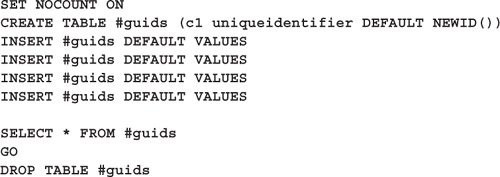
c1
------------------------------------
07A7DEFF-367F-11D3-92AC-005004044A19
07A7DF00-367F-11D3-92AC-005004044A19
07A7DF01-367F-11D3-92AC-005004044A19
07A7DF02-367F-11D3-92AC-005004044A19
Each table can have as many uniqueidentifier columns as you wish and can identify a single uniqueidentifier column as its ROWGUIDCOL column. The ROWGUIDCOL can be used to reference its corresponding uniqueidentifier column indirectly without actually naming it (analogously to IDENTITYCOL). Here’s an example:

SELECT ROWGUIDCOL FROM #guids
GO
DROP TABLE #guids
c1
------------------------------------
07A7DF1D-367F-11D3-92AC-005004044A19
07A7DF1E-367F-11D3-92AC-005004044A19
07A7DF1F-367F-11D3-92AC-005004044A19
07A7DF20-367F-11D3-92AC-005004044A19
Uniqueidentifiers have a number of disadvantages. Among them:
• Their values are unwieldy and cryptic. They’re random and don’t fit or match any sort of mnemonic pattern.
• The uniqueidentifier data type is four times as large as the four-byte int type that’s typically used for row identifiers. This makes accessing them slower in general, including building and accessing indexes over them.
• The sequence in which a set of uniqueidentifier values were generated is not discernable from the values themselves—you can’t tell which values came first and which ones came later by looking only at the data. Among other things, this means that they make poor ORDER BY columns.
A cursor variable stores a reference to a cursor definition. Cursors defined via variables are by definition local cursors (since you can’t declare global variables) and can be used in place of direct cursor references in commands such as OPEN, FETCH, CLOSE, and DEALLOCATE. They support the full Transact-SQL cursor syntax and can be used to define read-only as well as updatable cursors. Cursor variables and the cursor data type can be used most places ordinary variables and data types can with three exceptions:
• You can’t define a table column of type cursor.
• You can’t define stored procedure input parameters as cursors (but you can define cursor output parameters).
• You can’t assign a cursor variable with a SELECT statement. (They must be assigned using the SET command.)
Here’s an example of a simple cursor variable definition:
DECLARE @cursor CURSOR
SET @cursor=CURSOR FOR SELECT * FROM authors
OPEN @cursor
FETCH @cursor
WHILE (@@FETCH_STATUS=0) BEGIN
FETCH @cursor
END
CLOSE @cursor
DEALLOCATE @cursor
In this example, we define the cursor using the SET assignment statement. Cursor variables can also be assigned from existing cursors, like so:
DECLARE @cursor CURSOR
DECLARE c CURSOR FOR SELECT * FROM authors
SET @cursor=c
OPEN @cursor
FETCH @cursor
WHILE (@@FETCH_STATUS=0) BEGIN
FETCH @cursor
END
CLOSE @cursor
DEALLOCATE @cursor
DEALLOCATE c
Here, we first define the cursor using the traditional DECLARE CURSOR syntax; then we assign it by name to the cursor variable. Note the separate deallocation of the cursor variable and the cursor. Deallocating the cursor alone isn’t enough; it remains in memory until it’s explicitly deallocated or the last variable referencing it goes out of scope, whichever comes last. For example, consider this variation on the code:
DECLARE @cursor CURSOR
DECLARE c CURSOR FOR SELECT * FROM authors
SET @cursor=c
DEALLOCATE c
OPEN @cursor
FETCH @cursor
WHILE (@@FETCH_STATUS=0) BEGIN
FETCH @cursor
END
CLOSE @cursor
DEALLOCATE @cursor
Once you’ve assigned a regular cursor to a cursor variable, you can reference the cursor using either the original name or the variable—they’re almost synonymous. So, for example, once you’ve opened the cursor via the cursor variable, as in the last example, you can’t reopen it using the original cursor name without closing it first—it’s already open. Likewise, closing the cursor variable closes the original cursor, too—they refer to the same internal structure. As a rule, they’re interchangeable. The lone exception is the DEALLOCATE command.
As you can see from the example code, deallocating the original cursor doesn’t prevent you from continuing to access it via the cursor variable. Even though the code deallocates it immediately after assigning it to the cursor variable, it doesn’t actually go away. Deallocating a cursor reference other than the final one merely removes your ability to access the cursor via that reference—the cursor itself hangs around until the last variable referencing it is deallocated or goes out of scope.
You can define more than one cursor variable that references a particular cursor, and you can assign cursor variables to one another. Here’s an example:
DECLARE @cursor1 CURSOR, @cursor2 CURSOR
DECLARE c CURSOR FOR SELECT * FROM authors
SET @cursor1=c
SET @cursor2=@cursor1
OPEN @cursor2
FETCH @cursor2
WHILE (@@FETCH_STATUS=0) BEGIN
FETCH @cursor1
END
CLOSE @cursor1
DEALLOCATE @cursor1
DEALLOCATE @cursor2
DEALLOCATE c
One handy feature of Transact-SQL cursor variables is support for cursor output parameters. In the past, returning a cursor from a stored procedure meant either displaying it immediately or trapping it in a table via INSERT...EXEC. Cursor variables give you more control over when and whether to display a procedure’s result set. You can call FETCH to return the result set a row at a time or place it into a variable, or you can simply close and deallocate the cursor—it’s up to you.
Several of the system procedures that relate to cursors return cursor output parameters. Sp_describe_cursor, for example, returns a cursor that points to a single-row result set containing a report on the cursor you specify. This necessitates setting up a cursor variable and passing it into the procedure as an OUTPUT parameter, like so:
DECLARE @cursor CURSOR
DECLARE c CURSOR GLOBAL FOR SELECT * FROM authors
OPEN c
EXEC sp_describe_cursor @cursor_return=@cursor OUTPUT,
@cursor_source=N’global’,
@cursor_identity=N’c’
FETCH @cursor
FETCH c
WHILE (@@FETCH_STATUS=0) BEGIN
FETCH c
END
CLOSE @cursor
CLOSE c
DEALLOCATE @cursor
DEALLOCATE c
(Result set abridged)
reference_name cursor_name cursor_scope status model concurrency scrollable open_status cursor_rows
-------------- ----------- ------------ ------ ----- ----------- ---------- ----------- -----------
c c 2 1 3 3 0 1 -1
Once it processes the cursor, the code closes and deallocates the cursor along with its own global cursor. In this case, it can get away with making a single call to FETCH to return sp_describe_cursor’s one row. If the cursor returned by the stored procedure referenced a multirow result set, the code would need to loop through it, fetching each row separately. This call to sp_cursor_list illustrates:
DECLARE @authorcursor CURSOR, @authorcursor2 CURSOR, @cursorlist CURSOR
DECLARE AuthorsList CURSOR GLOBAL FOR SELECT * FROM authors
SET @authorcursor=AuthorsList
SET @authorcursor2=AuthorsList
OPEN AuthorsList
EXEC sp_cursor_list @cursor_return=@cursorlist OUTPUT,
@cursor_scope=3

Sp_cursor_list provides the same basic info as sp_describe_cursor but lists info for more than one cursor (all global cursors, all local cursors, or all cursors of either type). The cursor it returns via @cursorlist is fetched a row at a time until it’s fully retrieved; then the cursor is closed and deallocated as before.
Note that the prohibition against cursor input parameters means that a cursor output parameter may not have a cursor allocated to it prior to passing it to a procedure. If SQL Server permitted this, it would allow the input parameter restriction to be circumvented since an output parameter can be inspected and used just like any other stored procedure parameter. Here’s an example:
-- DON’T DO THIS -- BAD T-SQL
USE pubs
GO
IF (OBJECT_ID(’inputcursorparm’) IS NOT NULL)
DROP PROC inputcursorparm
GO
CREATE PROC inputcursorparm @cursor_input cursor VARYING OUT
AS
FETCH @cursor_input
WHILE (@@FETCH_STATUS=0) BEGIN
FETCH @cursor_input
END
CLOSE @cursor_input
DEALLOCATE @cursor_input
GO
DECLARE @c CURSOR
SET @c=CURSOR FOR SELECT * FROM authors
-- An error is generated when the procedure is called
-- because @c references an existing cursor
EXEC inputcursorparm @c OUT
Server: Msg 16951, Level 16, State 1, Line 7
The variable ’@c’ cannot be used as a parameter because a CURSOR OUTPUT parameter
must not have a cursor allocated to it before execution of the procedure.
Despite the name, timestamp columns have nothing to do with the time or date. A timestamp is a special binary(8) value that’s guaranteed to be unique across a database. A timestamp column is updated each time the data in a row changes. In SQL Server’s infancy, timestamp columns were used to effect a simplistic optimistic locking strategy that’s best explained by an example. If Juliet updates a row after Romeo reads it but before he posts his own changes, Romeo’s update attempt will fail because it will use the original timestamp value to try to locate the row. Romeo’s UPDATE statement will include the timestamp column in its WHERE clause but won’t be able to locate the original record because the timestamp value has changed due to Juliet’s update. This prevents Romeo from overwriting Juliet’s changes and provides a means for his application to detect that another user modified the row he was editing.
The TSEQUAL() function can be used to compare timestamp values. If the timestamps aren’t equal, TSEQUAL() raises an error and aborts the current command batch.
A table is limited to a single timestamp column. A common convention is to name the column timestamp, but that’s not required by the server. Here’s a code sample that shows how to use the timestamp data type:

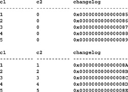
Note the different values for each row’s timestamp column before and after the UPDATE.
You can access the last generated timestamp value for a database via the @@DBTS automatic variable. Each database maintains its own counter, so be sure you’re in the correct database before querying @@DBTS. Here’s an example:
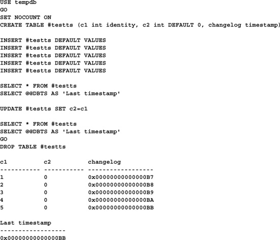
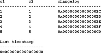
Note the USE tempdb at the first of the script. Since temporary tables reside in tempdb, we have to change the current database focus to tempdb in order for @@DBTS to work properly. @@DBTS always returns the last timestamp value generated for a database, so you can use it to acquire the timestamp of an update you’ve just performed, similar to the @@IDENTITY automatic variable. One big difference between @@DBTS and @@IDENTITY is that @@IDENTITY is connection specific whereas @@DBTS is database specific. The value returned by @@IDENTITY will rarely be the same for multiple users, but @@DBTS will often be identical for all users connected to a given database.
In this chapter you’ve explored SQL Server’s wealth of data types. You’ve learned about date, numeric, string, bit, and BLOB data types, as well as fringe types such as timestamps and uniqueidentifiers. Designing sound databases and writing robust Transact-SQL code require intimate familiarity with the wide variety of data types SQL Server provides. Knowing them well is the first step in writing optimal code to access them.