What Is Scaffolding?

Scaffolding is the process of filling missing rows of data within a data set to assist analysis. A data set may appear complete—with no nulls and a record for each individual entity—but still not be suited for the analysis you wish to conduct. Consider a mobile phone operator that wishes to analyze its monthly revenue from contracted customers. Figure 39-1 shows the data the operator is likely to have.

Figure 39-1. Data set requiring scaffolding to assist analysis

As you can see, the operator has a record of the customer, the contract start date, the contract length, and the monthly price for the service. However, there is no date to determine the value we’re seeking to analyze, monthly revenue. The only dates to use for analysis are the contract start date and end date. If the contract is for two years, we would need 24 records to gain full insight. As Figure 39-2 demonstrates, there is only a single month of revenue per Customer ID, and we can’t see the revenue being collected over time.

Figure 39-2. Resulting visualization from data set in Figure 39-1

Scaffolding is the answer to this problem. The technique adds a row for each of the “missing” records that are required for the analysis. In the mobile phone operator example, a scaffold would create the additional rows so each monthly payment would have its own record. The resulting data set would have a single row per contract, per month, for the cost of the service. This means there will be a row for each customer with an active contract per month. After 12 months, one contract is no longer active, and after 18 months, another ends. The scaffolding creates the data profile shown in Figure 39-3.

Figure 39-3. Profile of the scaffolded data in Prep Builder’s Profile pane

Giving all of the individual payments a row of their own in the data set allows analytical software, like Tableau Desktop, to show the full revenue over time. Figure 39-4 shows a sample of the resulting data set.

Figure 39-4. Sample of the scaffolded data set

Challenges Addressed by Scaffolding

Scaffolding techniques address several challenges, many of which are rapidly becoming more common due to subscription pricing—a payment schedule wherein the consumer pays a smaller amount on a regular basis rather than making a large one-time purchase. Subscription music, software, and food services are increasing in popularity, creating a bigger need for data analysts to be able to work with subscription data. Scaffolding goes beyond addressing the challenge of subscription-based data sets, however. It can also help in these areas:

Retention

Reporting on expected revenue can be presumptuous. Just because a customer signs up for a subscription-based product doesn’t mean that they will keep up those payments. Scaffolding can help you remove rows of projected revenues to more accurately determine levels of customer retention.

Inflation/exchange rates

Depending on the length of the subscription, you might need to account for factors like inflation or changing exchange rates in order to accurately represent earned revenue. Projecting these values is an art in its own right, but applying common forecasts with a scaffold can greatly improve the value of the analysis. Often projections will be stored in a secondary reference table and need to be joined onto the original data set along with the scaffold.

Data duplication

If you have fields that are aggregated over the periods covered in a record that you are then scaffolding out, you’ll need to divide these values over the number of periods to avoid duplicating the aggregations.

Challenges Created by Scaffolding

While the scaffolding technique does supply the additional rows of data required for analysis, it creates another challenge that should be considered.

Scaffolding will multiply the size of the data set you are analyzing considerably. This poses challenges for:

Data storage

The larger the data set, the greater the amount of storage that you will need.

Computing power

Not everyone has a brand new, powerful computer to use. Adding a huge number of rows to (potentially) an already large data set can really test your computer’s working memory.

Filtering at the data source level can significantly reduce the impact of scaffolding on your data size.

The Traditional Scaffolding Technique

Scaffolding has been used for a long time, and the traditional technique uses a scaffold of all possible values. Returning to the mobile provider example, we need to create a new Date field containing each month from the earliest contract start date in the data set to the latest contract end date (Figure 39-5).

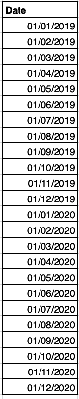
Figure 39-5. Data set to be used for scaffolding

As you can see, the longest contract starts in January 2019 and runs 24 months, so the latest date we need is December 2020. Just having the date range required isn’t sufficient, though. This scaffold needs to be joined to the customer data. To do this, we have two options:

• Create a calculation that defines the last month of the contract as End Date and then join using the conditions Start Date >= Scaffold Date and End Date <= Scaffold Date.

• Create a condition that will join each row in each data set together. This can then be filtered to remove any excess rows. The calculation that’s easiest to join is just the number 1. Create this calculation in each data set and join on a condition where 1 = 1 (i.e., every row joins to every other row). This is another style of appending, covered in Chapter 33.

The second join condition using 1 is easier to follow, as you can see the results of the join and filter to ensure each aspect is correct. Let’s follow that approach in the mobile provider example.

Step 1: Input the Data Sets

Input both data sets—Subscription Data and Scaffold (Figure 39-6).

Figure 39-6. Inputs for scaffolding

Step 2: Build the Join Calculations

Build a calculation of the value 1 in a Clean step. For simplicity’s sake, call the calculation “1” too (Figure 39-7).

Figure 39-7. Creating a calculation to act as the join condition

Repeat this step for both inputs (Figure 39-8).

Figure 39-8. Flow resulting from creating calculations to act as the join condition

Step 3: Join the Two Data Sets Together

Using a Join step, connect the two flows together using the join condition of 1 = 1 for an inner join (Figure 39-9).

Figure 39-9. Flow resulting from joining the Subscription Data and Scaffold data sets

This adds each row of a customer record from the Subscription Data set to each date. Prep clearly displays the results of this join in the lower part of the Join configuration pane (Figure 39-10).

Figure 39-10. Join Results section of the Join configuration pane

As there are 3 subscriptions recorded and 24 dates captured, the join produces 72 rows of data.

Step 4: Filter Out Unnecessary Rows

To be able to filter out any rows containing dates before the contract start date or after the contract expires, we first need to create a calculation for End Date. Add a new Clean step and create the calculation shown in Figure 39-11.

Figure 39-11. Adding an End Date calculation

This will add a new End Date field in your data set. You can easily check that it has worked as intended in Prep’s Profile pane (Figure 39-12).

Figure 39-12. Result of scaffold

Once you have the end date of the subscription, you can filter out the dates that have been added by the scaffold that fall outside the contract start and end dates. The calculation in Figure 39-13 uses the datetrunc() function to set the frequency of the scaffold. This data set is monthly, so we can ignore the day of the month as you will accrue revenue for the entire month when the contract starts and each month until it ends.

Figure 39-13. Calculation to retain only dates within the contract dates

A filter within a Clean step in Prep Builder must return a Boolean result. The records that meet the condition set—that is, those returning a True value—will remain in the data set. Those that do not meet the condition set in the filter—those returning False—will be removed from the flow, leaving one row per month of revenue per contract (Figure 39-14).

Figure 39-14. Row count demonstrating the correct outcome from the scaffolding

The Newer Scaffolding Technique

While the traditional technique works, it does have a number of shortcomings. The most notable of these is that the list of dates in the scaffold has to be maintained and updated. This doesn’t sound too problematic, but it means remembering where the file is kept, remembering to update it, and making sure your colleagues also know where and how to do this (in case you leave).

This all changed when Bethany Lyons presented a new technique in Tableau Desktop at a Tableau conference a few years ago. Her approach resolved many of these issues by challenging the logic that a data set that needs to be scaffolded to create extra records for each date. Like the traditional method just detailed, the new technique utilizes different date calculations, but it differs in that they are all created from simple integers. In the mobile provider example, the longest contract length is 24 months, so the scaffold would require a column of integers from 0 to 23 (Figure 39-15).

Figure 39-15. Data set for the newer scaffold technique

Let’s look in more detail at the differences in this technique and how it addresses the shortcomings of the traditional scaffolding approach.

Step 2: Join the Data Sets

This time, instead of 1 = 1, we set the join condition as Scaffold < Contract Length (Figure 39-16). This means that a scaffold row will be assigned to each subscription up to the point where the scaffold number is the same as the contract length. This works because the values in the scaffold start at 0 (we’ll get to that shortly).

Figure 39-16. Setup of the join between the data set and new scaffold

Notice how the number of rows required is already correct, so there is no need to filter later in the flow. This is a massive advantage when you have thousands or millions of customers, since you aren’t adding millions of rows only to remove them straightaway.

Step 3: Add the Reporting Date

In the previous technique, the scaffold date became the date used for reporting. As no such date exists this time, we need to create it. We use the dateadd() function, setting Start Date as the contract start date and Scaffold as the increment on top of this (Figure 39-17).

Figure 39-17. Creating the reporting date with the new scaffold

As the first scaffold value is 0, we don’t need to increment the contract start date further. Any subsequent increment adds the level of date part applied. Because the mobile contract payments are monthly, we set the dateadd() level as 'month'. Another advantage of this technique is that the date returned is much more likely to be when the revenue is actually collected by the provider (Figure 39-18).

Figure 39-18. Result of the scaffold

The Result

You can generate the visualization of all monthly revenues in Tableau Desktop after outputting the data. In Figure 39-19, the Customer ID has been added so it’s easier to see the effect of the multiple rows (one per month) of the scaffolding.

Figure 39-19. Updated visualization resulting from scaffolded data set

You should now be able to easily apply scaffolding to any data set that lacks full monthly records. This technique has enabled a lot of analytical solutions that would not have been possible otherwise.

Summary

For Desktop users who need to add all possible dates into a data set in order to analyze the data correctly, scaffolding is a good solution. Using Prep to avoid applying this technique in Desktop can simplify the analytical process for end users. Further use cases for scaffolding include dividing targets across multiple dates or carefully filling in missing values in the data (you’ll need to disclose to end users that these are estimates). Now that you know the core techniques, you’ll be able to approach these additional challenges with confidence.