
11. Project Design in Action
The difficulty facing many project design novices is not the specific design techniques and concepts, but rather the end-to-end flow of the design process. It is also easy to get mired in the details and to lose sight of the objective of the design effort. Without experience, you may be stumped when you encounter the first snag or situation that does not behave as prescribed. It is impractical to try to cover all possible contingencies and responses. Instead, it is better to master the thought process involved in project design.
This chapter demonstrates the thought process and the mindset via a comprehensive walkthrough of the design effort. The emphasis is on the systematic examination of the steps and iterations. You will see observations and rules of thumb, how to alternate between project design options, how to home in on what makes sense, and how to evaluate tradeoffs. As this chapter evolves, it demonstrates ideas from the previous chapters as well as the synergy gained by combining project design techniques. It also covers additional aspects of project design such as planning assumptions, complexity reduction, staffing and scheduling, accommodating constraints, compression, and risk and planning. As such, the objective of this chapter is teaching project design flow and techniques, as opposed to providing a real-life example.
The Mission
Your mission is to design a project to build a typical business system. This system was designed using The Method, but that fact is immaterial in this chapter. In general, the input to the project design effort should include the following ingredients:
The static architecture. You use the static architecture to create the initial list of coding activities.
Call chains or sequence diagrams. You produce the call chains or sequence diagrams by examining the use cases and how they propagate through the system. These provide the rough cut of structural activity dependencies.
List of activities. You list all activities, coding and noncoding alike.
Duration estimation. For each activity, you accurately estimate the duration (and resources) involved (or work with others to do so).
Planning assumptions. You capture the assumptions you have about staffing, availability, ramp-up time, technology, quality, and so on. You typically will have several such sets of assumptions, with each set resulting in a different project design solution.
Some constraints. You write down all the explicitly known constraints. You should also include possible or likely constraints, and plan accordingly. You will see multiple examples in this chapter for handling constraints.
The Static Architecture
Figure 11-1 shows the static architecture of the system. As you can tell, the system is fairly limited in size. It includes two Clients, five business logic components, three ResourceAccess components, two Resources, and three Utilities.

Figure 11-1 The system static architecture
While the system in Figure 11-1 was inspired by a real system, the merits of this particular architecture are irrelevant in this chapter. When designing the project, you should avoid turning the project design effort into a system design review. Even poor architectures should have adequate project design to maximize the chance of meeting your commitments.
The Call Chains
The system has only two core use cases and two call chains. The first call chain, shown in Figure 11-2, concludes with publishing an event. The second call chain in Figure 11-3, depicts the processing of that event by the subscribers.

Figure 11-2 Call chain 1

Figure 11-3 Call chain 2
Dependency Chart
You should examine the call chains, and lay out a first draft of the dependencies between components in the architecture. You start with all the arrows connecting components, regardless of transport or connectivity, and consider each as a dependency. You should account for any dependency exactly once. However, typically the call chain diagrams do not show the full picture because they often omit repeated implicit dependencies. In this case, all components of the architecture (except the Resources) depend on Logging, and the Clients and Managers depend on the Security component. Armed with that additional information, you can draw the dependency chart shown in Figure 11-4.

Figure 11-4 Initial dependency chart
As you can see, even with a simple system having only two use cases, the dependency chart is cluttered and hard to analyze. A simple technique you can leverage to reduce the complexity is to eliminate dependencies that duplicate inherited dependencies. Inherited dependencies are due to transitive dependencies1—those dependencies that an activity implicitly inherits by depending on other activities. In Figure 11-4, Client A depends on Manager A and Security; Manager A also depends on Security. This means you can omit the dependency between Client A and Security. Using inherited dependencies, you can reduce Figure 11-4 to Figure 11-5.

Figure 11-5 Dependency chart after consolidating inherited dependencies
List of Activities
While Figure 11-5 is certainly simpler than Figure 11-4, it is still inadequate because it is highly structural in nature, showing only the coding activities. You must compile a comprehensive list of all activities in the project. In this case, the list of noncoding activities includes additional work on requirements, architecture (such as technology verification or a demo service), project design, test plan, test harness, and system testing. Table 11-1 lists all activities in the project, their duration estimation, and their dependencies on preceding activities.
Table 11-1 Activities, duration, and dependencies
ID |
Activity |
Duration (days) |
Depends On |
|---|---|---|---|
1 |
Requirements |
15 |
|
2 |
Architecture |
20 |
1 |
3 |
Project Design |
20 |
2 |
4 |
Test Plan |
30 |
3 |
5 |
Test Harness |
35 |
4 |
6 |
Logging |
15 |
3 |
7 |
Security |
20 |
3 |
8 |
Pub/Sub |
5 |
3 |
9 |
Resource A |
20 |
3 |
10 |
Resource B |
15 |
3 |
11 |
ResourceAccess A |
10 |
6,9 |
12 |
ResourceAccess B |
5 |
6,10 |
13 |
ResourceAccess C |
15 |
6 |
14 |
Engine A |
20 |
12,13 |
15 |
Engine B |
25 |
12,13 |
16 |
Engine C |
15 |
6 |
17 |
Manager A |
20 |
7,8,11,14,15 |
18 |
Manager B |
25 |
7,8,15,16 |
19 |
Client App1 |
25 |
17,18 |
20 |
Client App2 |
35 |
17 |
21 |
System Testing |
30 |
5,19,20 |
Network Diagram
With the list of activities and dependencies at hand, you can draw the project network as an arrow diagram. Figure 11-6 shows the initial network diagram. The numbers in this figure correspond to the activity IDs in Table 11-1. The bold lines and numbers indicate the critical path.

Figure 11-6 Initial network diagram
About Milestones
As defined in Chapter 8, a milestone is an event in the project denoting the completion of a significant part of the project, including major integration achievements. Even at this early stage in the project design, you should designate the event completing Project Design (activity 3) as the SDP review milestone, M0. In this case, M0 is the completion of the front end (short for fuzzy front end) of the project, comprising requirements, architecture, and project design. This makes the SDP review an explicit part of the plan. You can have milestones on or off the critical path, and they can be public or private. Public milestones demonstrate progress for management and customers, while private milestones are internal hurdles for the team. If a milestone is outside the critical path, it is a good idea to keep it private since it could move as a result of a delay somewhere upstream from it. On the critical path, milestones can be both private and public, and they correlate directly with meeting the commitments of the project in terms of both time and cost. Another use for milestones is to force a dependency even if the call chains do not specify such a dependency. The SDP review is such a milestone—none of the construction activities should start before the SDP review. Such forced-dependency milestones also simplify the network, and you will see another example shortly.
Initial Duration
You can construct the network of activities listed in Table 11-1 in a project planning tool, which gives you a first look at project duration. Doing so gives a duration of 9.0 months for this project. However, without resource assignment, it is not yet possible to determine the cost of the project.
Planning Assumptions
To proceed with the design, you itemize the planning assumptions, especially the planned staffing requirements, in a list such as the following:
One project manager is required throughout the project.
One product manager is required throughout the project.
One architect is required throughout the project.
One developer is required per service for any coding activity. Once that service is complete, the developer can move to another activity.
One database architect is required for each of the Resources. This work is independent of the code development work and can be done in parallel.
One tester is required from the start of construction of the system services until the end of testing.
One additional tester is required during system testing.
One test engineer is required for the test plan and test harness activities.
One DevOps specialist is required from the start of construction until the end of testing.
This list is, in fact, the list of resources you need to complete the project. Also note the structure of the list: “one X for Y.” If you cannot state the required staffing this way, you probably do not understand your own staffing requirements, or you are missing a key planning assumption.
You should explicitly make two additional planning assumptions about the developers regarding testing time and idle time. First, in this example project, developers will produce such high-quality work that they will not be needed during system testing. Second, developers between activities are considered a direct cost. Strictly speaking, idle time should be accounted for as an indirect cost because it is not associated with project activities, yet the project must pay for it. However, many project managers strive to assign idle developers some activities in support of other development activities, even if that means more than one developer is temporarily assigned per service. Under this planning assumption, you still account for developers between activities as direct cost.
Project Phases
Each activity in a project always belongs to a phase, or a type of activities. Typical phases include the front end, design, infrastructure, services, UI, testing, and deployment, among others. A phase may contain any number of activities, and the activities in a phase can overlap on the timeline. What is less obvious is that the phases are not sequential and can themselves overlap or even start and stop. The easiest way of laying out phases is to structure the planning assumptions list into a role/phase table; Table 11-2 provides an example.
Table 11-2 Roles and phases
Role |
Front End |
Infrastructure |
Services |
Testing |
|---|---|---|---|---|
Architect |
X |
X |
X |
X |
Project Manager |
X |
X |
X |
X |
Product Manager |
X |
X |
X |
X |
DevOps |
|
X |
X |
X |
Developers |
|
X |
X |
|
Testers |
|
|
X |
X |
In much the same way, you could add other roles that are required for the duration of an entire phase, such as UX (user experience) or security experts. However, you should not include roles that are required only for specific activities, such as the test engineer.
Table 11-2 is a crude form of a staffing distribution view. The relationship between roles and phases is essential when building the staffing distribution chart because you must account for the use of all the resources, regardless of whether they are assigned to specific project activities. For example, in Table 11-2, an architect is required throughout the project. In turn, in the staffing distribution chart, you would show the architect across the duration of the project. In this way, you can account for all resources necessary to produce the correct staffing distribution chart and cost calculation.
Finding the Normal Solution
With the list of activities, dependencies, and planning assumptions in hand, you proceed to iteratively find the normal solution. For the first pass, assume that you have unlimited resources at your disposal, but you will utilize only as many resources as required to progress unimpeded along the critical path. This provides the least constrained way of building the system at the lowest level of resources.
Unlimited Resources (Iteration 1)
Initially, also assume that you have unlimited staffing elasticity. You could make very minor (if any) adjustments for reality. For example, there is no point in hiring a person for a single week if you can trade some float and avoid any need for that resource. You assume that every special skill set is available when needed. These liberal assumptions should yield the same project duration as you had before assigning resources. Indeed, after staffing the project this way, the duration remains at 9.0 months and yields the planned earned value chart shown in Figure 11-7. This chart exhibits the general shape of a shallow S curve but it is not as smooth as it should be.

Figure 11-7 Planned earned value with unlimited resources
Following the process outlined in Chapter 7, Figure 11-8 shows the corresponding project staffing distribution chart. This plan uses as many as four developers and two database architects, uses one test engineer, and does not consume any float. The calculated project total cost is 58.3 man-months.

Figure 11-8 Staffing distribution with unlimited resources
Recall from Chapter 9 that finding the normal solution is an iterative process (see Figure 9-8) simply because the lowest level of staffing is not known at the beginning of the design effort. Therefore, this first set of results is not yet the normal solution. In the next iteration you should accommodate reality, consume float to decrease staffing volatility, address any obvious design flaws, and reduce complexity if possible.
Network and Resource Problems
The first iteration on the normal solution suffers from several key problems. First, it assumes unlimited and readily available resources, including those with special skills. Clearly, resources are not limitless, and special skills are rare. Second, the planned staffing distribution chart (see Figure 11-8) displays a concerning sign (identified in Chapter 7)—namely, a high ramp coming into the project. You should expect this behavior due to the assumptions about staffing availability and elasticity. Third, over its duration, the project engages some resources only for short periods of time. This is asking for trouble as far as availability and necessary onboarding time. While you could plan to mitigate that by using subcontractors, you should not create problems that you need to solve. The staffing distribution should be smooth, and you should avoid high ramps and sharp drops. You should create other project variations that have some resource constraints and entertain a more realistic staffing elasticity. Often, this will also smooth both the staffing distribution and the planned earned value charts.
The last problem with the solution so far is the integration pressure on the Manager services. From Table 11-1 and the network diagram of Figure 11-6, you can see that the Managers (activities 17 and 18) are expected to integrate with four or five other services. Ideally, you should integrate only one or two services at a time. Integrating more than two services concurrently will likely result in a nonlinear increase in complexity because any issues across services will be superimposed on each other. The problem is further compounded because the integrations occur toward the end of the project, when you have little runway left to fix issues.
Infrastructure First (Iteration 2)
A common technique to simplify the project is to move the infrastructure services (Utilities such as Logging, Security, and Pub/Sub, and any additional infrastructure activity such as build automation) to the beginning of the project, regardless of their natural dependencies in the network. In other words, immediately after M0, the developers will work on these infrastructure services. You can even introduce a milestone called M1 denoting when the infrastructure is complete, making all other services depend on M1, as shown in the subnetwork in Figure 11-9.

Figure 11-9 Infrastructure first
Completing the infrastructure first reduces the complexity in the network (decreases the number of dependencies and crossing lines) and alleviates the integration pressure at the Managers. Overriding the original dependencies in this way typically reduces the initial staffing demand because none of the other services can start until M1 is complete. It also reduces the staffing volatility and usually results in a smoother staffing distribution and a gradual ramp-up at the beginning of the project.
Another important advantage of developing the infrastructure first is the early access it provides to key infrastructure components. This allows developers to integrate their work with the infrastructure as they construct the system, rather than having to retrofit and test infrastructure services (such as Logging or Security) after the fact. Having the infrastructure services available before the business-related components (ResourceAccess, Engines, Managers, and Clients) is almost always an excellent idea, even if the need is not evident at first.
Developing the infrastructure first changes the initial staffing to three developers (one per service) until after M1, at which point the project can absorb a fourth developer (note you are still working on an staffing plan with unlimited resources). Repeating the prior steps, the infrastructure first plan extends the schedule by 3% to 9.2 months and incurs 2% of additional total cost, to 59 man-months. In exchange for the negligible additional cost and schedule, the project gains early access to key services and a simpler, more realistic plan. Going forward, this new project becomes the baseline for the next iteration.
Limited Resources
The resources you ask for may not always be available when you need them, so it is prudent to plan for fewer resources (at least initially) to mitigate that risk. How will the project behave if three developers are unavailable at the beginning of the project? If no developers at all are available, the architect can develop the infrastructure, or the project can engage subcontractors: The infrastructure services do not require domain knowledge, so they are good candidates for such external and readily available resources. If only one developer is available at the beginning, then that single developer can do all infrastructure components serially. Perhaps only a single developer is available initially, and then a second developer can join in after the first activity is complete.
Infrastructure First with Limited Resources (Iteration 3)
Choosing the latter, somewhat middle-of-the-road scenario of one and then two developers, recalculate the infrastructure-first project to see how the project behaves with limited resources. Instead of three parallel activities (one critical) at the beginning, as shown in Figure 11-9, you now have one activity that is critical, then two activities in parallel (one critical). Serializing activities in this way increases the duration of the project. This variation extends the schedule by 8% to 9.9 months and increases the total cost by 4% to 61.5 man-months. Figure 11-10 shows the resulting staffing distribution chart. Note the gradual phasing in of the developers, from one, to two, to four.

Figure 11-10 Staffing distribution of infrastructure-first with limited resources
Extending the critical path by limiting the resources also increases the float of the noncritical activities that span that section of the network. Compared with unlimited resources, the float of the Test Plan (activity 4 in Figure 11-6) and Test Harness (activity 5 in Figure 11-6) is increased by 30%, the float of Resource A (activity 9 in Figure 11-6) is increased by 50%, and the float of Resource B (activity 10 in Figure 11-6) is increased by 100%. This is noteworthy because a seemingly minute change in resource availability has increased the float dramatically. Be aware that this knife can cut both ways: Sometimes a seemingly innocuous change can cause the floats to collapse and derail the project.
No Database Architects (Iteration 4)
On top of limiting the initial availability of the developers, suppose the project did not get the database architects called for in the previous solutions. This is certainly a real-life scenario—such qualified resources are often hard to come by. In this case, developers design the databases to the best of their abilities. To see how the project responds to this new limit, instead of just adding developers, constrain the project to no more than four developers (allowing for more developers would be identical to having the database architects). Surprisingly, this does not change the duration and results with a total cost of 62.7 man-months, a mere 2% increase. The reason is that the same four developers start working earlier and do not even have to consume float.
Further Limited Resources (Iteration 5)
Since the project could easily cope with four developers, the next limited-resources plan caps the available developers at three. This also does not change the duration of the project because it is possible to trade the fourth developer for some float. As for cost, there is a 3% reduction in cost to 61.1 man-months due to the more efficient use of developers. Figure 11-11 shows the resulting staffing distribution chart.

Figure 11-11 Staffing distribution with three developers and one test engineer
Note the use of the test engineer along with the three developers. Figure 11-11 is the best staffing distribution so far, looking very much like the expected pattern from Chapter 7 (see Figure 7-8).
Figure 11-12 shows the shallow S curve of the planned earned value. The figure shows a fairly smooth shallow S curve. If anything, the shallow S is almost too shallow. You will see the meaning of that later on.

Figure 11-12 Planned earned value with three developers and one test engineer
Figure 11-13 shows the corresponding network diagram, using the absolute criticality float color-coding scheme described in Chapter 8. This example project uses 9 days as the upper limit for red activities and 26 days as the upper limit for the yellow activities. The activity IDs appear above the arrows in black, and the float values are shown below the line in the arrow’s color. The test engineer’s activities—that is, the Test Plan (activity 4) and the Test Harness (activity 5)—have a very high float of 65 days. Note the M0 milestone terminating the front end and the M1 milestone at the end of the infrastructure. The diagram also shows the phasing in of the resources between M0 and M1 to build the infrastructure (activities 6, 7, and 8).

Figure 11-13 Network diagram with three developers and one test engineer
No Test Engineer (Iteration 6)
The next experiment in resource reduction is to remove the test engineer but keep the three developers. Once again, this design solution results in no change to the duration and cost of the project. The third developer simply takes over the test engineer’s activities after completing other lower-float activities already assigned. The problem is that deferring the Test Plan and Test Harness activities to much later consumes 77% of their float (from 65 days to 15 days). This is very risky because if the float drops by 100%, the project is delayed.
Going Subcritical (Iteration 7)
Chapter 9 explained the importance of presenting the effects of subcritical staffing to decision makers. Too often, decision makers are unaware of the impracticality of cutting back on resources to supposedly reduce costs. The example project becomes subcritical by limiting the number of developers to just two and eliminating the test engineer. By the time activities on the critical path are scheduled to start, some supporting noncritical activities are not ready yet, so they impede the old critical path. The limiting factor now is not the duration of the critical path, but rather the availability of the two developers. Consequently, the old network (and specifically the old critical path) no longer applies. You must therefore redraw the network diagram to reflect the dependency on the two developers.
Recall from Chapter 7 that resource dependencies are dependencies and that the project network is a dependency network, not just an activity network. You therefore add the dependency on the resources to the network. You actually have some flexibility in designing the network: As long as the natural dependency between the activities is satisfied, the actual order of the activities can vary. To create the new network, you assign the two resources, as always, based on float. Each developer takes on the next lowest-float activity available after finishing with the current activity. At the same time, you add a dependency between the developer’s next activity and the current one to reflect the dependency on the developer. Figure 11-14 shows the subcritical network diagram for the example project.

Figure 11-14 Subcritical solution network diagram
Given that only two developers are performing most of the work, the subcritical network diagram looks like two long strings. One string of activities is the long critical path; the other string is the second developer back-filling on the side. This long critical path increases the risk to the project because the project now has more critical activities. In general, subcritical projects are always high-risk projects.
In the extreme case of having only a single developer, all activities in the project are critical, the network diagram is one long string, and the risk is 1.0. The duration of the project equates to the sum of all activities, but, due to the maximum risk, even that duration is likely to be exceeded.
Subcritical Cost and Duration
Compared with the limited-resources solution of three developers and one test engineer, the project duration is extended by 35% to 13.4 months due to the serialization of the activities. While using a smaller development team, the project total cost is increased by 25% to 77.6 man-months due to the longer duration and the mounting indirect cost. This result clearly demonstrates the point: There really is no cost saving with subcritical staffing.
Planned Earned Value
Figure 11-15 shows the subcritical planned earned value. You can see that the supposed shallow S curve is almost a straight line.

Figure 11-15 Subcritical planned earned value
In the extreme case of only a single developer doing all the work, the planned earned value is a straight line. In general, a lack of curvature in the planned earned value chart is a telltale sign for a subcritical project. Even the somewhat anemic shallow S curve in Figure 11-12 indicates the project is close to becoming subcritical.
Choosing the Normal Solution
The search for the normal solution has involved several attempts using combinations of resources and network designs. Out of all of these, the best solution so far was Iteration 5 (which relied on three developers and one test engineer) for several reasons:
This solution complies with the definition of the normal solution by utilizing the lowest level of resources that allows the project to progress unimpeded along the critical path.
This solution works around limitations of access to experts such as database architects while not compromising on a key resource, the test engineer.
This solution does not expect all the developers to start working at once.
Both the staffing distribution chart and the planned earned value chart exhibit acceptable behavior.
The front end of this solution encompasses, as expected, 25% of the duration of the project, and the project has an acceptable efficiency of 23%. Recall from Chapter 7 that the efficiency number should not exceed 25% for most projects.
The rest of the chapter uses Iteration 5 as the normal solution and as the baseline for the other iterations. Table 11-3 summarizes the various project metrics of the normal solution.
Table 11-3 Project metrics of the normal solution
Project Metric |
Value |
|---|---|
Total cost (man-months) |
61.1 |
Direct cost (man-months) |
21.8 |
Duration (months) |
9.9 |
Average staffing |
6.1 |
Peak staffing |
9 |
Average developers |
2.3 |
Efficiency |
23% |
Front End |
25% |
Network Compression
With the normal solution in place, you can try to compress the project and see how well certain compression techniques work. There is no single correct way of compressing a project. You will have to make assumptions about availability, complexity, and cost. Chapter 9 discussed a variety of compression techniques. In general, the best strategy is to start with the easier ways of compressing the project. For demonstration purposes, this chapter shows how to compress the project using several techniques. Your specific case will be different. You may choose to apply only a few of the techniques and the ideas discussed here, weighing carefully the implications of each compressed solution.
Compression Using Better Resources
The simplest way of compressing any project is to use better resources. This requires no changes to the project network or the activities. Although the simplest form of compression, it may not be the easiest due to the availability of such resources (more on that in Chapter 14). The purpose here is to gauge how the project will respond to compressing with better resources, or even if it is worth pursuing, and, if it is, how to do so.
Compression Using a Top Developer (Iteration 8)
Suppose you have access to a top developer who can perform coding activities 30% faster than the developers you already have. Such a top developer is likely to cost much more than 30% of the cost of a regular developer. In this project you can assume the top developer costs 80% more than a regular developer.
Ideally you would assign such a resource only on the critical path, but that is not always possible (recall the discussion of task continuity from Chapter 7). The normal baseline solution assigns two developers to the critical path, and your goal is to replace one of them with the top resource. To identify which one, you should consider both the number of activities and the number of days spent on the critical path per person.
Table 11-4 lists the two developers in the normal solution who touch the critical path, the number of critical activities versus noncritical activities each has, and the total duration on the critical path and off the critical path. Clearly, it is best to replace Developer 2 with the top developer.
Table 11-4 Developers, critical activities, and duration
Resource |
Noncritical Activities |
Noncritical Duration (days) |
Critical Activities |
Critical Duration (days) |
|---|---|---|---|---|
Developer 1 |
4 |
85 |
2 |
35 |
Developer 2 |
1 |
5 |
4 |
95 |
Next, you need to revisit Table 11-1 (the duration estimations for each activity), identify the activities for which Developer 2 is responsible, and adjust their duration downward by 30% (the expected productivity gain with the better resource) using 5-day resolution. With the new activity durations, repeat the project duration and cost analysis while accounting for the additional 80% markup for Developer 2.
Figure 11-16 shows the critical path on the network diagram before and after compressing with the top developer.

Figure 11-16 New critical path with one top developer
The new project duration is 9.5 months, only 4% shorter than the duration of the original normal solution. The difference is so small because a new critical path has emerged, and that new path holds the project back. Such miniscule reduction in duration is a fairly common result. Even if that single resource is vastly more productive than the other team members, and even if all activities assigned to that top resource are done much faster, the durations of the activities assigned to regular team members are unaffected by the top resource, and those activities simply stifle the compression.
In terms of cost, the compressed project cost is unchanged, despite having a top resource that costs 80% more. This, too, is expected because of the indirect cost. Most software projects have a high indirect cost. Reducing the duration even by a little tends to pay for the cost of compression, at least with the initial compression attempts, because the minimum of the total cost curve is to the left of the normal solution (see Figure 9-10).
Compression Using a Second Top Developer (Iteration 9)
You could try compressing with multiple top resources. In this example, it makes sense to ask for just a second top developer to replace Developer 1 because a third top developer could be assigned only outside the critical path. With a second top resource, the compression has a more noticeable effect: The schedule is reduced by an additional 11% to 8.5 months, and the total cost is reduced by 3% to 59.3 man-months.
Introducing Parallel Work
Often, the only meaningful way of accelerating projects is to introduce parallel work. There are multiple ways of working in parallel in a software project, some more challenging than others. Parallel work increases the project complexity, so here too you should consider the simplest and easiest techniques first.
Low-Hanging Fruit
The best candidates for parallel work in most well-designed systems are the infrastructure and the Client designs because both are independent of the business logic. Earlier, you saw this independence play out in Iteration 2, which pushed the infrastructure to start immediately after the SDP review. To enable parallel work with the Clients, you split the Clients into separate design and development activities. Such Client-related design activities typically include the UX design, the UI design, and the API or SDK design (for external system interactions). Splitting the Clients also supports better separation of Client designs from the back-end system because the Clients should provide the best experience for the consumers of the services, not merely reflect the underlying system. You can now move the infrastructure development and the Client design activities to be parallel to the front end.
This move has two downsides, however. The lesser downside is the higher initial burn rate, which increases simply because you need developers as well as the core team at the beginning. The larger downside is that starting the work before the organization is committed to the project tends to make the organization decide to proceed, even if the smart thing to do is to cancel the project. It is human nature to disregard the sunk cost or to have an anchoring bias2 attached to shining UI mockups.
2. https://en.wikipedia.org/wiki/Anchoring
I recommend moving the infrastructure and the Client designs to the front end only if the project is guaranteed to proceed and the purpose of the SDP review is solely to select which option to pursue (and to sign off on the project). You could mitigate the risk of biasing the SDP decision by moving only the infrastructure development to be in parallel to the front end, proceeding with the Client designs after the SDP review. Finally, make sure that the Client design activities are not misconstrued as significant progress by those who equate UI artifacts with progress. You should combine the work in the front end with project tracking (see Appendix A) to ensure decision makers correctly interpret the status of the project.
Adding and Splitting Activities
Identifying additional opportunities for parallel work is more challenging elsewhere in the project. You have to be creative and find ways of eliminating dependencies between coding activities. This almost always requires investing in additional activities that enable parallel work such as emulators, simulators, and integration activities. You also have to split activities and extract out of them new activities for the detailed design of contracts, interfaces, messages or the design of dependent services. These explicit design activities will take place in parallel to other activities.
There is no set formula for this kind of parallel work. You could do it for a few key activities or for most activities. You could perform the additional activities up-front or on-the-go. Very quickly you will realize that eliminating all dependencies between coding activities is practically impossible because there are diminishing returns on compression when all paths are near-critical. You will be climbing the direct cost curve of the project, which, near the minimum duration point (see Figure 9-3), is characterized by a steep slope, requiring even more cost for less and less reduction in schedule.
Infrastructure and Client Designs First (Iteration 10)
Returning to the example, the next iteration of project design compression moves the infrastructure in parallel to the front end. It also splits the Client activities into some up-front design work (e.g., requirements, test plan, UI design) and actual Client development, and moves the Client designs to the front end. In this example project you can assume that the Client design activities are independent of the infrastructure and are unique per Client.
Table 11-5 lists the revised set of activities, their duration, and their dependencies for this compression iteration.
Table 11-5 Activities with infrastructure and Client designs first
ID |
Activity |
Duration (days) |
Depends On |
|---|---|---|---|
1 |
Requirements |
15 |
|
2 |
Architecture |
20 |
1 |
3 |
Project Design |
20 |
2 |
4 |
Test Plan |
30 |
22 |
5 |
Test Harness |
35 |
4 |
6 |
Logging |
10 |
|
7 |
Security |
15 |
6 |
8 |
Pub/Sub |
5 |
6 |
9 |
Resource A |
20 |
22 |
10 |
Resource B |
15 |
22 |
11 |
ResourceAccess A |
10 |
9,23 |
12 |
ResourceAccess B |
5 |
10,23 |
13 |
ResourceAccess C |
10 |
22,23 |
14 |
EngineA |
15 |
12,13 |
15 |
EngineB |
20 |
12,13 |
16 |
EngineC |
10 |
22,23 |
17 |
ManagerA |
15 |
14,15,11 |
18 |
ManagerB |
20 |
15,16 |
19 |
Client App1 |
15 |
17,18,24 |
20 |
Client App2 |
20 |
17,25 |
21 |
System Testing |
30 |
5,19,20 |
22 |
M0 |
0 |
3 |
23 |
M1 |
0 |
7,8 |
24 |
Client App1 Design |
10 |
|
25 |
Client App2 Design |
15 |
|
Note that Logging (activity 6), and therefore the rest of the infrastructure activities, along with the new Client design activities (activities 24 and 25), can start at the beginning of the project. Note also that the actual Client development activities (activities 19 and 20) are shorter now and depend on the completion of the respective Client design activities.
Several potential issues arise when compressing this project by moving the infrastructure and the Client design activities to the front end. The first challenge is cost. The duration of the front end now exceeds the duration of the infrastructure and the Client design activities, even when done serially by the same resources. Therefore, starting that work simultaneously with the front end is wasteful because the developers will be idle toward the end. It is more economical to defer the start of the infrastructure and the Client designs until they become critical. This will increase the risk of the project, but reduce the cost while still compressing the project.
In this iteration, you can reduce the cost further by using the same two developers to develop the infrastructure first; after completing the infrastructure, they follow with the Client design activities. Since resource dependencies are dependencies, you make the Client design activities depend on the completion of the infrastructure (M1). To maximize the compression, the two developers used in the front end proceed to other project activities (the Resources) immediately after the SDP review (M0). In this specific case, to calculate the floats correctly, you also make the SDP review dependent on the completion of the Client design activities. This removes the dependency on the Client design activities from the Clients themselves and allows the Clients to inherit the dependency from the SDP review instead. Again, you can afford to override the dependencies of the network in this case only because the front end is longer than the infrastructure and the Client design activities combined. Table 11-6 shows the revised dependencies of the network (changes noted in red).
Table 11-6 Revised dependencies with infrastructure and Client designs first
ID |
Activity |
Duration (days) |
Depends On |
|---|---|---|---|
1 |
Requirements |
15 |
|
… |
… |
… |
… |
19 |
Client App1 |
15 |
17,18,24 |
20 |
Client App2 |
20 |
17,25 |
21 |
System Testing |
30 |
5,19,20 |
22 |
M0 |
0 |
3,24,25 |
23 |
M1 |
0 |
7,8 |
24 |
Client App1 Design |
10 |
23 |
25 |
Client App2 Design |
15 |
23 |
The other challenge with splitting activities is the increased complexity of the Clients as a whole. You could compensate for that complexity by assigning the Client design activities and development to the same two top developers from the previous compression iteration. This compounds the effect of compression with top resources. However, since the Clients and the project are now more complex and demanding, you should further compensate for that by assuming there is no 30% reduction in the time it takes to build the Clients (but the developers still cost 80% more). These compensations are already reflected in the duration estimation of activities 19 and 20 in Table 11-5 and Table 11-6.
The result of this compression iteration is a cost increase of 6% from the previous solution to 62.6 man-months and a schedule reduction of 8% to 7.8 months. Figure 11-17 shows the resulting network diagram.

Figure 11-17 Network diagram for infrastructure and Client designs first
Compression with Simulators (Iteration 11)
Examining Figure 11-17 reveals that a near-critical path (activities 10, 12, 15, 18, and 19) has developed alongside the critical path. This means any further compression requires compressing both of these paths to a similar degree. Compressing just one of them will have little effect because the other path then dictates the duration of the project. In this kind of situation, it is best to look for a crown—that is, a large activity that sits on top of both paths. Compressing the crown compresses both paths. In this example project, the best candidates are the development of the Client apps (activities 19 and 20) and the Manager services (activities 17 and 18). The Clients and Managers are relatively large activities, and they crown both paths. You could try to compress the Clients, the Managers, or both.
Compressing the Clients becomes possible when you develop simulators (see Chapter 9) for the Manager services on which they depend and move the development of the Clients somewhere upstream in the network, in parallel to other activities. Since no simulator is ever a perfect replacement for the real service, you also need to add explicit integration activities between the Clients and the Managers, once the Managers are complete. This in effect splits each Client development into two activities: The first is a development activity against the simulators, and the second is an integration activity against the Managers. As such, the Clients development may not be compressed, but the overall project duration is shortened.
You could mimic this approach by developing simulators for the Engines and ResourceAccess services on which the Managers depend, which enables development of the Managers earlier in the project. However, in a well-designed system and project, this would usually be far more difficult. Although simulating the underlying services would require many more simulators and make the project network very complex, the real issue is timing. The development of these simulators would have to take place more or less concurrently with the development of the very services they are supposed to simulate, so the actual compression you can realize from this approach is limited. You should consider simulators for the inner services only as a last resort.
In this example project, the best approach is to simulate the Managers only. You can compound the previous compression iteration (infrastructure and Client designs at the front end) by compressing it with simulators. A few new planning assumptions apply when compressing this iteration:
Dependencies. The simulators could start after the front end, and they also require the infrastructure. This is inherited with a dependency on
M0(activity 22).Additional developers. When using the previous compression iteration as the starting point, two additional developers are required for the development of simulators and the Client implementations.
Starting point. It is possible to reduce the cost of the two additional developers by deferring the work on the simulators and the Clients until they become critical. However, networks containing simulators tend to be fairly complex. You should compensate for that complexity by starting with the simulators as soon as possible and have the project benefit from higher float as opposed to lower cost.
Table 11-7 lists the activities and the changes to dependencies, while using the previous iteration as the baseline solution and incorporating its planning assumptions (changes noted in red).
Table 11-7 Activities with Manager simulators
ID |
Activity |
Duration (days) |
Depends On |
|---|---|---|---|
1 |
Requirements |
15 |
|
… |
… |
… |
… |
17 |
ManagerA |
15 |
… |
18 |
ManagerB |
20 |
… |
19 |
Client App1 Integration |
15 |
17,18,28 |
20 |
Client App2 Integration |
20 |
17,29 |
… |
… |
… |
… |
26 |
ManagerA Simulator |
15 |
22 |
27 |
ManagerB Simulator |
20 |
22 |
28 |
Client App1 |
15 |
26,27 |
29 |
Client App2 |
20 |
26 |
Figure 11-18 shows the resulting staffing distribution chart. You can clearly see the sharp jump in the developers after the front end and the near-constant utilization of the resources. The average staffing in this solution is 8.9 people, with peak staffing of 11 people. Compared with the previous compression iteration, the simulators solution results in a 9% reduction in duration to 7.1 months, but increases the total cost by only 1% to 63.5 man-months. This small cost increase is due to the reduction in the indirect cost and the increased efficiency and expected throughput of the team when working in parallel.

Figure 11-18 The simulators solution staffing distribution chart
Figure 11-19 shows the simulators solution network diagram. You can see the high float for the simulators (activities 26 and 27) and Client development (activities 28 and 29). Also observe that virtually all other network paths are critical or near critical and there is high integration pressure toward the end of the project. This solution is fragile to the unforeseen, and the network complexity drastically increases the execution risk.

Figure 11-19 The simulators solution network diagram
End of Compression Iterations
Compared with the normal solution, the simulators solution reduces the schedule by 28% while increasing the cost by only 4%. Due to the high indirect cost, the compression ends up practically paying for itself. The direct cost, by comparison, increases by 59%, twice the reduction in the duration from a percentage standpoint. As noted in Chapter 9, the maximum expected compression of a software project is at most 30%, making the simulators solution as compressed as this project is ever likely to get.
While further compression is theoretically possible (by compressing the Managers), in practice this is as far as the project design team should go. There is a low probability of success from compressing any further, and the core team will be wasting time designing improbable projects.
Throughput Analysis
It is important to recognize how compression affects the expected throughput of the team compared with the normal solution. As explained in Chapter 7, the pitch of the shallow S curve represents the throughput of the team. Figure 11-20 plots the shallow S curves of the planned earned value for the normal solution and each of the compressed solutions on the same scale.

Figure 11-20 Planned earned value of the project solutions
As expected, the compressed solutions have a steeper shallow S since they complete sooner. You can quantify the difference in the required throughput by replacing each curve with its respective linear regression trend line and examining the equation of the line (see Figure 11-21).

Figure 11-21 Earned value trend lines for the project solutions
The trend lines are straight lines, so the coefficient of the x term is the pitch of the line and, therefore, the expected throughput of the team. In the case of the normal solution, the team is expected to operate at 39 units of productivity, while the simulators solution calls for 59 units of productivity (0.0039 versus 0.0059, scaled to integers). The exact nature of these units of productivity is immaterial. What is important is the difference between the two solutions: The simulators solution expects a 51% increase in the throughput of the team (59 – 39 = 20, which is 51% of 39). It is unlikely that any team, even by increasing its size, could increase its throughput by such a large factor.
Although not a hard-and-fast rule, comparing the ratio of average-to-peak staffing from one solution to another can give you some sense whether the throughput difference is realistic. For the simulators solution, this ratio is 81%, compared to 68% for the normal solution; in other words, the simulators solution expects more intense utilization of the resources. Since the simulators solution also requires a larger average team size (8.9 versus 6.1 of the normal solution) and since larger teams tend to be less efficient, the prospect of achieving the 51% increase in throughput is questionable, especially when working on a more complex project. This further cements the idea that the simulators solution is a bar set too high for most teams.
Efficiency Analysis
The efficiency of each project design solution is a fairly easy number to calculate—and a very telling one. Recall from Chapter 7 that the efficiency number indicates both the expected efficiency of the team and how realistic the design assumptions are regarding constraints, staffing elasticity, and criticality of the project. Figure 11-22 shows the project solutions efficiency chart for the example project.

Figure 11-22 The project efficiency chart
Observe in Figure 11-22 that peak efficiency is at the normal solution, resulting from the lowest level of resources utilization without any compression cost. As you compress the project, efficiency declines. While the simulators solution is on par with the normal solution, I consider it unrealistic since the project is much more complex and its feasibility is in question (as indicated by the throughput analysis). The subcritical solution is awful when it comes to efficiency due to the poor ratio of direct cost to the indirect cost. In short, the normal solution is the most efficient.
Time–Cost Curve
Having designed each solution and produced its staffing distribution chart, you can calculate the cost elements for each solution, as shown in Table 11-8.
Table 11-8 Duration, total cost, and cost elements for the various options
Design Option |
Duration (months) |
Total Cost (man-months) |
Direct Cost (man-months) |
Indirect Cost (man-months) |
|---|---|---|---|---|
Simulators |
7.1 |
63.5 |
34.8 |
28.7 |
Infra+Clients Front End |
7.8 |
62.6 |
30.4 |
32.2 |
TopDev1+TopDev2 |
8.5 |
59.3 |
26.6 |
32.7 |
TopDev2 |
9.5 |
61.1 |
24.2 |
36.9 |
Normal |
9.9 |
61.1 |
21.8 |
39.2 |
Subcritical |
13.4 |
77.6 |
20.9 |
56.7 |
With these cost numbers, you can produce the project time–cost curves shown in Figure 11-23. Note that the direct cost curve is a bit flat due to the scaling of the chart. The indirect cost is almost a perfect straight line.
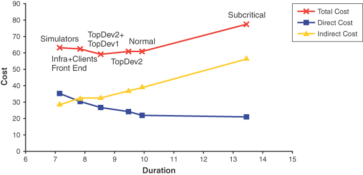
Figure 11-23 The project time–cost curves
Time–Cost Correlation Models
The time–cost curves of Figure 11-23 are discrete, and they can only hint at the behavior of the curves outside the specific solutions. However, with the discrete time–cost curves at hand, you can also find correlation models for the curves. A correlation model or a trend line is a mathematical model that produces a curve that best fits the distribution of the discrete data points (tools such as Microsoft Excel can easily perform such analysis). Correlation models allow you to plot the time–cost curves at any point, not just at the known discrete solutions. For the points in Figure 11-23, these models are a straight line for the indirect cost, and a polynomial of the second degree for the direct and indirect costs. Figure 11-24 shows these correlation trend lines in dashed lines, along with their equations and R2 values.

Figure 11-24 The project time–cost trend lines
The R2 (also known as the coefficient of determination) is a number between 0 and 1 that represents the quality of the model. Numbers greater than 0.9 indicate an excellent fit of the model to the discrete points. In this case, the equations within the range of the project design solutions depict their curves very precisely.
Figure 11-24 provides the equations for how cost changes with time in the example project. For the direct and indirect costs, the equations are:
where t is measured in months. While you also have a correlation model for the total cost, that model is produced by a statistical calculation, so it is not a perfect sum of the direct and indirect costs. You produce the correct model for the total cost by simply adding the equations of the direct and indirect models:
Figure 11-25 plots the modified total cost correlation model along with the direct and indirect models.

Figure 11-25 The project time–cost models
The Death Zone
Chapter 9 introduced the concept of the death zone—that is, the area under the time–cost curve. Any project design solution that falls in that area is impossible to build. Having the model (or even the discrete curve) for the project total cost enables you to visualize the project death zone, as shown in Figure 11-26.

Figure 11-26 The project death zone
Identifying the death zone allows you to answer intelligently quick questions and avoid committing to impossible projects. For example, suppose management asks if you could build the example project in 9 months with 4 people. According to the total cost model of the project, a 9-month project costs more than 60 man-months and requires an average of 7 people:
Assuming the same ratio of average-to-peak staffing as the normal solution (68%), a solution that delivers at 9 months peaks at 10 people. Any fewer than 10 people causes the project at times to go subcritical. The combination of 4 people and 9 months (even when utilized at 100% efficiency 100% of the time) is 36 man-months of cost. That particular time–cost coordinate is not even visible in Figure 11-26 because it is so deep within the death zone. You should present these findings to management and ask if they want to commit under these terms.
Planning and Risk
Each project design solution carries some level of risk. Using the risk modeling techniques described in Chapter 10, you can quantify these risk levels for the solutions, as shown in Table 11-9.
Table 11-9 Risk levels of the various options
Design Option |
Duration (months) |
Criticality Risk |
Activity Risk |
|---|---|---|---|
Simulators |
7.1 |
0.81 |
0.76 |
Infra+Clients Front End |
7.8 |
0.77 |
0.81 |
TopDev1+TopDev2 |
8.5 |
0.79 |
0.80 |
TopDev2 |
9.5 |
0.70 |
0.77 |
Normal |
9.9 |
0.73 |
0.79 |
Subcritical |
13.4 |
0.79 |
0.79 |
Figure 11-27 plots the risk levels of the project design options along with the direct cost curve. The figure offers both good and bad news regarding risk. The good news is that criticality risk and activity risk track closely together in this project. It is always a good sign when different models concur on the numbers, giving credence to the values. The bad news is that all project design solutions so far are high-risk options; even worse, they are all similar in value. This means the risk is elevated and uniform regardless of the solution. Another problem is that Figure 11-27 contains the subcritical point. The subcritical solution is definitely a solution to avoid, and you should remove it from this and any subsequent analysis.

Figure 11-27 Direct cost and risk of the various options
In general, you should avoid basing your modeling on poor design options. To address the high risk, you should decompress the project.
Risk Decompression
Since in this example project all project design solutions are of high risk, you should decompress the normal solution and inject float along the critical path until the risk drops to an acceptable level. Decompressing a project is an iterative process because you do not know up front by how much to decompress or how well the project will respond to decompression.
Somewhat arbitrarily, the first iteration decompresses the project by 3.5 months, from the 9.9 months of the normal solution to the furthest point of the subcritical solution. This result reveals how the project responds across the entire range of solution durations. Doing so produces a decompression point called D1 (total project duration of 13.4 months) with criticality risk of 0.29 and activity risk of 0.39. As explained in Chapter 10, 0.3 should be the lowest risk level for any project, which implies this iteration overly decompressed the project.
The next iteration decompresses the project by 2 months from the normal duration, roughly half the decompression amount of D1. This produces D2 (total project duration of 12 months). The criticality risk is unchanged from 0.29, because these 2 months of decompression are still larger than the lower limit used in this project for green activities. Activity risk is increased to 0.49.
Similarly, halving the decompression of D2 yields D3 with a 1-month decompression (total project duration of 10.9 months), criticality risk of 0.43, and activity risk of 0.62. Half of D3 produces D4, a 2-week decompression (total project duration of 10.4 months) with criticality risk of 0.45 and activity risk at 0.7. Figure 11-28 plots the decompressed risk curves for the project.

Figure 11-28 Risk decompression curves
Adjusting Outliers
Figure 11-28 features a conspicuous gap between the two risk models. This difference is due to a limitation of the activity risk model—namely, the activity risk model does not compute the risk values correctly when the floats in the project are not spread uniformly (see Chapter 10 for more details). In the case of the decompressed solutions, the high float values of the test plan and the test harness skew the activity risk values higher. These high float values are more than one standard deviation removed from the average of all the floats, making them outliers.
When computing activity risk at the decompression points, you can adjust the input by replacing the float of the outlier activities with the average of all floats plus one standard deviation of all floats. Using a spreadsheet, you can easily automate the adjustment of the outliers. Such an adjustment typically makes the risk models correlate more closely.
Figure 11-29 shows the adjusted activity risk curve along with the criticality risk curve. As you can see, the two risk models now concur.

Figure 11-29 Criticality and adjusted activity risk decompression curves
Risk Tipping Point
The most important aspect of Figure 11-29 is the risk tipping point around D4. Decompressing the project even by a little to D4 decreases the risk substantially. Since D4 is right at the edge of the tipping point, you should be a bit more conservative and decompress to D3 to pass the knee in the curves.
Direct Cost and Decompression
To compare the decompressed solutions to the other solutions, you need to know their respective cost. The problem is that the decompression points provide only the duration and the risk. No project design solutions produce these points—they are just the risk value of the normal solution network with additional float. You have to extrapolate both the indirect and direct cost of the decompressed solutions from the known solutions.
In this example project, the indirect cost model is a straight line, and you can safely extrapolate the indirect cost from that of the other project design solution (excluding the subcritical solution). For example, the extrapolation for D1 yields an indirect cost of 51.1 man-months.
The direct cost extrapolation requires dealing with the effect of delays. The additional direct cost (beyond the normal solution that was used to create the decompressed solutions) comes from both the longer critical path and the longer idle time between noncritical activities. Because staffing is not fully dynamic or elastic, when a delay occurs, it often means people on other chains are idle, waiting for the critical activities to catch up.
In the example project’s normal solution, after the front end, the direct cost mostly consists of developers. The other contributors to direct cost are the test engineer activities and the final system testing. Since the test engineer has very large float, you can assume that the test engineer will not be affected by the schedule slip. The staffing distribution for the normal solution (shown in Figure 11-11) indicates that staffing peaks at 3 developers (and even that peak is not maintained for long) and goes as low as 1 developer. From Table 11-3, you can see that the normal solution uses 2.3 developers, on average. You can therefore assume that the decompression affects two developers. One of them consumes the extra decompression float, and the other one ends up idle.
The planning assumptions in this project stipulate that developers between activities are accounted for as a direct cost. Thus, when the project slips, the slip adds the direct cost of two developers times the difference in duration between the normal solution and the decompression point. In the case of the furthest decompression point D1 (at 13.4 months), the difference in duration from the normal solution (at 9.9 months) is 3.5 months, so the additional direct cost is 7 man-months. Since the normal solution has 21.8 man-months for its direct cost, the direct cost at D1 is 28.8 man-months. You can add the other decompression points by performing similar calculations. Figure 11-30 shows the modified direct-cost curve along with the risk curves.

Figure 11-30 Modified direct cost curve and the risk curves
Rebuilding the Time–Cost Curve
With the new cost numbers for D1, you can rebuild the time–cost curves, while excluding the bad data point of the subcritical solution. This yields a better time–cost curve based on possible solutions. You can then proceed to calculate the correlation models as before. This process produces the following cost formulas:
These curves have a R2 of 0.99, indicating an excellent fit to the data points. Figure 11-31 shows the new time–cost curves models as well as the points of minimum total cost and the normal solution.

Figure 11-31 Rebuilt time–cost curve models
With a better total cost formula now known, you can calculate the point of minimum total cost for the project. The total cost model is a second order polynomial of the form:
Recall from calculus that the minimum point of such a polynomial is when its first derivative is zero:
As discussed in Chapter 9, the point of minimum total cost always shifts to the left of the normal solution. While the exact solution of minimum total cost is unknown, Chapter 9 suggested that for most projects finding that point is not worth the effort. Instead, you can, for simplicity’s sake, equate the total cost of the normal solution with the minimum total cost for the project. In this case, the minimum total cost is 60.3 man-months and the total cost of the normal solution according to the model is 61.2 man-months, a difference of 1.5%. Clearly, the simplification assumption is justified in this case. If minimizing the total cost is your goal, then both the normal solution and the first compression solution with a single top developer are viable options.
Minimum Direct Cost
Following similar steps with the direct cost formula, you can easily calculate the point in time of minimum direct cost as 10.8 months. Ideally, the normal solution is also the point of minimum direct cost. In the example project, however, the normal solution is at 9.9 months. The discrepancy is partially due to the differences between a discrete model of the project and the continuous model (see Figure 11-30, where the normal solution is also minimum direct cost, versus Figure 11-31). A more meaningful reason is that the point has shifted due to rebuilding the time–cost curve to accommodate the risk decompression points. In practice, the normal solution is often offset a little from the point of minimum direct cost due to accommodating constraints. The rest of this chapter uses the duration of 10.8 months as the exact point of minimum direct cost.
Modeling Risk
You can now create trend line models for the discrete risk models, as shown in Figure 11-32. In this figure, the two trend lines are fairly similar. The rest of the chapter uses the activity risk trend line because it is more conservative: It is higher across almost all of the range of options.

Figure 11-32 The project time–risk trend lines
Fitting a polynomial correlation model, you now have a formula for risk in the project:
where t is measured in months.
With the risk formula you can plot the risk model side by side with the direct cost model, as in Figure 11-33.

Figure 11-33 Risk and direct cost models
Minimum Direct Cost and Risk
As mentioned earlier, the minimum of the direct cost model is at 10.8 months. Substituting that time value into the risk formula yields a risk value of 0.52; that is, the risk at the point of minimum direct cost is 0.52. Figure 11-33 visualizes this with the dashed blue lines.
Recall from Chapter 10 that ideally the minimum direct cost should be at 0.5 risk and that this point is the recommended decompression target. The example project is off that mark by 4%. While this project does not have project design solution with a duration of exactly 10.8 months, the known D3 decompression point comes close, with a duration of 10.9 months (see the dashed red lines in Figure 11-33). In a practical sense, these points are identical.
Optimal Project Design Option
The risk model value at D3 is at 0.50, meaning that D3 is the ideal target of risk decompression as well as practically the point of minimum direct cost. This makes D3 the optimal point in terms of direct cost, duration, and risk. The total cost at D3 is only 63.8 man-months, virtually the same as the minimum total cost. This also makes D3 the optimal point in terms of total cost, duration, and risk.
Being the optimal point means that the project design option has the highest probability of delivering on the commitments of the plan (the very definition of success). You should always strive to design around the point of minimum direct cost. Figure 11-34 visualizes the float of the project network at D3. As you can see, the network is a picture of health.

Figure 11-34 Float analysis of the optimal design solution
Minimum Risk
Using the risk formula, you can also calculate the point of minimum risk. This point comes at 12.98 months and a risk value of 0.248. Chapter 10 explained that the minimum risk value for the criticality risk model is 0.25 (using the weights [1, 2, 3, 4]). While 0.248 is very close to 0.25, it was produced using the activity risk formula, which, unlike the criticality risk model, is unaffected by the choice of weights.
Risk Inclusion and Exclusion
The discrete risk curve of Figure 11-29 indicates that while compression shortens the project, it does not necessarily increase the risk substantially. Compressing this example project even reduced the risk a bit on the activity risk curve. The main increase in risk was due to moving left of D3 (or minimum direct cost), and all compressed solutions have high risk.
Using the risk model, Figure 11-35 shows how all the project design solutions map to the risk curve of the project. You can see that the second compressed solution is almost at maximum risk, and that the more compressed solutions have the expected decreased level of risk (the da Vinci effect introduced in Chapter 10). Obviously, designing anything to or past the point of maximum risk is ill advised. You should avoid even approaching the point of maximum risk for the project—but where is that cutoff point? The example project has a maximum risk value of 0.85 on the risk curve, so project design solutions approaching that number are not good options. Chapter 10 suggested 0.75 as the maximum level of risk for any solution. With risk higher than 0.75, the project is typically fragile and likely to slip the schedule.

Figure 11-35 All design solutions and risk
Using the risk formula, you will find that the point of 0.75 risk is at duration of 9.49 months. While no project design solution exactly matches this point, the first compression point has a duration of 9.5 months and risk of 0.75. This suggests that the first compression is the upper practical limit in this example project. As discussed previously, 0.3 should be the lowest level of risk, which excludes the D1 decompression point at 0.27 risk. The D2 decompression point at 0.32 is possible, but borderline.
SDP Review
All the detailed project design work culminates in the SDP review, where you present the project design options to the decision makers. You should not only drive educated decisions, but also make the right choice obvious. The best project design option so far was D3, a one-month decompression offering both minimum cost and risk of 0.50.
When presenting your results to decision makers, list the first compression point, the normal solution, and the optimal one-month decompression from the normal solution. Table 11-10 summarizes these viable project design options.
Table 11-10 Viable project design options
Design Option |
Duration (months) |
Total Cost (man-months) |
Risk |
|---|---|---|---|
One Top Developer |
9.5 |
61.1 |
0.75 |
Normal Solution |
9.9 |
61.1 |
0.68 |
One-Month Decompression |
10.9 |
63.8 |
0.50 |
Presenting the Options
You should not actually present the raw information as shown in Table 11-10. It is unlikely that anyone has ever seen this level of precision, so you will lack credibility. You should also add the subcritical solution. Since the subcritical solution ends up costing more (as well as being risky and taking longer), you want to dispel such notions as early as possible.
Table 11-11 lists the project options you should present at the SDP review. Note the rounded schedule and cost numbers. The rounding was performed with a bit of a license to create a more prominent spread. While this will not change anything in the decision-making process, it does lend more credibility to the numbers.
Table 11-11 Project design options for review
Project Option |
Duration (months) |
Total Cost (man-months) |
Risk |
|---|---|---|---|
One Top Developer |
9 |
61 |
0.75 |
Normal Solution |
10 |
62 |
0.68 |
One-Month Decompression |
11 |
64 |
0.50 |
Subcritical Staffing |
13 |
77 |
0.78 |
The risk numbers are not rounded because risk is the best way of evaluating the options. It is nearly certain that the decision makers have never seen risk in a quantified form as a tool for driving educated decisions. You must explain to them that the risk values are nonlinear; that is, using the numbers from Table 11-11, 0.68 risk is a lot more risky than 0.5 risk, not a mere 36% increase. To illustrate nonlinear behavior, you can use an analogy between risk and a more familiar nonlinear domain, the Richter scale for earthquake strength. If the risk numbers were levels of earthquakes on the Richter scale, an earthquake of 6.8 is 500 times more powerful than an earthquake of 5.0 magnitude, and a 7.5 quake is 5623 times more powerful. This sort of plain analogy steers the decision toward the desired point of 0.50 risk.