
Chapter 2: Working with Data in PROC SQL
The SELECT Statement and Clauses
Date and Time Column Definitions
SQL Operators, Functions, and Keywords
Character String Operators and Functions
Dictionary Tables and Metadata
Displaying Dictionary Table Definitions
Accessing a Dictionary Table’s Contents
PROC SQL is essentially a database language as opposed to a procedural or computational language. This chapter’s focus is on working with data in PROC SQL using the SELECT statement. Often referred to as an SQL query, the SELECT statement is the most versatile statement in SQL and is used to read data from one or more database tables (or data sets). It also supports numerous extensions including keywords, operators, functions, and predicates, and returns the data in a table-like structure called a result-set.
The SELECT statement’s purpose is to retrieve (or read) data from the underlying tables (or views). Although it supports multiple clauses, the SELECT statement has only one clause that is required to be specified – the FROM clause. All the remaining clauses, described below, are optional and only used when needed. Note: Not every query needs to have all the clauses specified, but SQL provides developers and data analysts with a powerful and flexible language to access, manipulate, and display data without the need to write large amounts of code.
During execution, SAS carries out the tasks associated with planning, optimizing, and performing the operations specified in the SELECT statement and its clauses to produce the desired results. To prevent syntax errors from occurring when using the SELECT statement, the clauses must be specified in the correct order. To help you remember the order of the SELECT statement’s clauses recite, “SQL is fun when geeks help others.” The first letter in each word corresponds to the name of the SELECT statement’s clause as shown in Figure 2.1.
Figure 2.1: Order of the SELECT Statement Clauses

When constructed correctly, the SELECT statement and its clauses declares the database table (or data set) to find the data in, what data to retrieve, and whether any special transformations or processing is needed before the data is returned. The next example shows the correct syntax of a query’s SELECT statement and its clauses.
SQL Code
PROC SQL;
SELECT PRODNAME
,PRODTYPE
,PRODCOST
INTO :M_PRODNAME
,:M_PRODTYPE
,:M_PRODCOST
FROM PRODUCTS
WHERE PRODNAME CONTAINS "Software"
GROUP BY PRODTYPE
HAVING COUNT(PRODTYPE) > 3
ORDER BY PRODNAME;
QUIT;
Results

Now that we’ve explored the order that each clause is specified in an SQL query, let’s examine the order of execution of each clause in an SQL query. Table 2.1 illustrates and describes the execution order of each SELECT statement clause.
Table 2.1: Clause Execution Order
|
Clause Execution Order |
Description |
|
1. FROM Clause |
The first clause executed in a query is the FROM clause. It is a required clause with the purpose of determining the working set of data that is being queried (i.e., variable names, variable type, number of rows, and other important information). |
|
2. INTO Clause |
The INTO clause is used to create one or more macro variables where the values can be used to manipulate data in DATA and PROC steps. |
|
3. WHERE Clause |
The WHERE clause is used to subset rows of data based on the condition(s) specified, and rows that aren’t satisfied by the condition(s) are discarded. |
|
4. GROUP BY Clause |
The GROUP BY clause takes the rows that were subset with the WHERE clause and grouped based on common values in the column specified in the GROUP BY clause. |
|
5. HAVING Clause |
The HAVING clause applies the condition(s) to the grouped rows specified in the GROUP BY clause, and any grouped rows that aren’t satisfied by the condition(s) are discarded. |
|
6. SELECT Statement |
Expressions specified in the SELECT statement are processed. |
|
7. ORDER BY Clause |
The ORDER BY clause sorts the rows of data in either ascending (default) or descending order. |
The purpose of a database is to store data. A database contains one or more tables (and other components). Tables consist of columns and rows of data. In the SAS implementation of SQL, the available data types are limited to only two possibilities:
● numeric
● character
The SAS implementation of SQL provides programmers with numerous arithmetic, statistical, and summary functions. It offers one numeric data type to represent numeric data. Columns defined as a numeric data type with the NUMERIC or NUM column definition are assigned a default length of 8 bytes, even if the column is created with a numeric length of less than 8 bytes. This provides the greatest degree of precision allowed by SAS software. In the example, a table called PURCHASES is created consisting of four numeric columns. The resulting table contains no rows of data, as illustrated by the SAS log results. For more information about the CREATE TABLE statement, see Chapter 5, “Creating, Populating, and Deleting Tables.”
SQL Code
PROC SQL;
CREATE TABLE PURCHASES
(CUSTNUM NUM,
PRODNUM NUM,
UNITS NUM,
UNITCOST NUM(8,2));
QUIT;
SAS Log Results
PROC SQL;
CREATE TABLE PURCHASES
(CUSTNUM NUM,
PRODNUM NUM,
UNITS NUM,
UNITCOST NUM(8,2));
NOTE: Table PURCHASES created, with 0 rows and 4 columns.
QUIT;
Results

Creating a numeric column that is less than 8 bytes requires the use of the DATA step LENGTH statement. Although it is not necessary to assign smaller lengths to numeric columns because it can result in precision issues, doing so can make for more efficient use of data storage system resources. The example illustrates a DATA step that assigns smaller lengths to the four numeric variables in the PURCHASES table: CUSTNUM, PRODNUM, UNITS, and UNITCOST. In contrast to the SAS log results produced by the previous PROC SQL code, the CONTENTS output illustrates the creation of a data set with one record and four user-defined, and shorter length, numeric variables.
DATA Step Code
DATA PURCHASES;
LENGTH CUSTNUM 4.
PRODNUM 3.
UNITS 3.
UNITCOST 4.;
LABEL CUSTNUM = ‘Customer Number’
PRODNUM = ‘Product Purchased’
UNITS = ‘# Units Purchased’
UNITCOST = ‘Unit Cost’;
FORMAT UNITCOST DOLLAR12.2;
RUN;
PROC CONTENTS DATA=PURCHASES;
RUN;
SAS Log Results
DATA PURCHASES;
LENGTH CUSTNUM 4.
PRODNUM 3.
UNITS 3.
UNITCOST 4.;
LABEL CUSTNUM = 'Customer Number'
PRODNUM = 'Product Purchased'
UNITS = '# Units Purchased'
UNITCOST = 'Unit Cost';
FORMAT UNITCOST DOLLAR12.2;
RUN;
NOTE: Variable CUSTNUM is uninitialized.
NOTE: Variable PRODNUM is uninitialized.
NOTE: Variable UNITS is uninitialized.
NOTE: Variable UNITCOST is uninitialized.
NOTE: The data set WORK.PURCHASES has 1 observations and 4 variables.
NOTE: DATA statement used:
real time 2.80 seconds
PROC CONTENTS DATA=PURCHASES;
RUN;
NOTE: PROCEDURE CONTENTS used:
real time 1.82 seconds
CONTENTS Results
In the next example, a LENGTH= modifier is illustrated in the PROC SQL code to assign smaller lengths to the four numeric variables (columns) in the PURCHASES table: CUSTNUM, PRODNUM, UNITS, and UNITCOST.
PROC SQL Code
PROC SQL;
CREATE TABLE PURCHASES
(CUSTNUM NUM LENGTH=4
LABEL=’Customer Number’,
PRODNUM NUM LENGTH=3
LABEL=’Product Purchased’,
UNITS NUM LENGTH=3
LABEL=’# Units Purchased’,
UNITCOST NUM LENGTH=4
LABEL=’Unit Cost’);
QUIT;
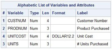
As shown in the CONTENTS results below, four numeric columns are defined using a LENGTH= column modifier that is smaller than the default length of 8 bytes.
CONTENTS Results

Database application processing stores date and time information in the form of a numeric data type. Date and time values are represented internally as an offset where a SAS date value is stored as the number of days from the fixed date value of 01/01/1960 (January 1, 1960). The SAS date value for January 1, 1960, is represented as 0 (zero). A date earlier than this date is represented as a negative number and a date later than this date is represented as a positive number. This makes performing date calculations much easier.
SAS has integrated the vast array of date and time informats and formats with PROC SQL. The various informats and formats act as input and output templates and describe how date and time information is to be read or rendered on output. See the SAS Language Reference: Dictionary for detailed descriptions of the various informats and formats and their use. Numeric date and time columns, when combined with informats and/or formats, automatically validate values according to the following rules:
● Date—Date informats and formats enable PROC SQL and SAS to determine the month, day, and year values of a date. The month value handles values from 1 through 12. The day value handles values from 1 through 31 and applies additional validations to a maximum of 28, 29, or 30 depending on the month in question. The year value handles values from 1 through 9999. Dates go back to 1582 and ahead to 20,000. When you enter a year value of 0001 and specify a format and a Yearcutoff value of 1920, the returned value would be 2001.
● Time —Time informats and formats enable PROC SQL to determine the hour, minute, and second values of a time. The hour portion handles values from 00 through 23. The minute portion handles values from 00 through 59. The second portion handles values from 00 through 59.
● DATETIME—Date and time stamps enable the SQL procedure to determine the month, day, and year of a date as well the hour, minute, and second of a time.
See Chapter 5, “Creating, Populating, and Deleting Tables” and Chapter 6, “Modifying and Updating Tables and Indexes” for more information about date and time informats and formats.
PROC SQL provides tools to manipulate and store character data including words, text, and codes using the CHARACTER or CHAR data type. The characters allowed by this data type include the ASCII or EBCDIC character sets. The CHARACTER or CHAR data type stores fixed-length character strings consisting of a maximum of 32K characters. If a length is not specified, a CHAR column stores a default of 8 characters.
The SQL programmer has a vast array of SQL and Base SAS functions that can make the task of working with character data considerably easier. In this chapter, you’ll learn how columns based on the character data type are defined, and how string functions, pattern matching, phonetic matching techniques, and a variety of other techniques are used with character data.
Missing values are an important aspect when dealing with data. The concept of missing values is familiar to programmers, statisticians, researchers, and other SAS users. This chapter describes what NULL values are, what they aren’t, and how they are used.
Missing or unknown information is supported by PROC SQL in a form known as a null value. A null value is not the same as a zero value. In SAS, null values are treated as a separate category from known values. A value consisting of zero has a known value. In contrast, a value of null has an unknown quantity and will never be known. For example, a patient who is given an eye exam does not have zero eyesight just because the results from the exam haven’t been received. The correct value to assign in a case like this is a missing or a null value.
In another example, say a person declines to provide their age on a survey. This person’s age is null, not zero. Essentially, this person has an age, but it is unknown. Whenever an unknown value occurs, you have no choice but to assign an unknown value—null.
Because the value of null is unknown, any arithmetic calculation using a null will return a null. This makes a lot of sense because the results of a calculation using a null are not determinable. This is sometimes referred to as the propagation of nulls because when a null value is used in a calculation or an expression, it propagates a null value. For example, if a null is added to a known value, then the result is a null value.
In SAS, a numeric data type containing a null value (absence of any value) is represented with a period (.). This representation indicates that the column has not been assigned a value. A null value has no value and is not the same as zero. A value consisting of zero has a known quantity as opposed to a null value that is not known and never will be known.
If a null value is multiplied with a known value, the result is a null value represented with a period (.). In the next example, when UNITS and UNITCOST both have known values, their product will generate a known value, as illustrated below.
SQL Code
PROC SQL;
SELECT CUSTNUM,
PRODNUM,
UNITS,
UNITCOST,
UNITS * UNITCOST AS Total FORMAT=DOLLAR12.2
FROM PURCHASES
ORDER BY Total;
QUIT;
Results


SQL provides three keywords: AS, DISTINCT, and UNIQUE to perform specific operations on the results. Each will be presented in order as follows.
Creating Column Aliases
In situations where data is computed using system functions, statistical functions, or arithmetic operations, a column name or header can be left blank. To prevent this from occurring, users may specify the AS keyword to provide a name to the column or heading itself along with formatting directions. The next example illustrates using the AS keyword to prevent the name for the computed column from being assigned a temporary column name similar to _TEMAxxx. The name assigned with the AS keyword is also used as the column header on output, as shown below.
SQL Code
PROC SQL;
SELECT PRODNAME,
PRODTYPE,
PRODCOST * 0.80 AS Discount_Price FORMAT=DOLLAR9.2
FROM PRODUCTS
ORDER BY 3;
QUIT;
Results

Finding Duplicate Values
In some situations, several rows in a table may contain identical or duplicate column values. To select only one of each identical or duplicate values, SAS supports and processes the DISTINCT and UNIQUE keywords the same and without any noticeable performance differences. On another note, the ANSI standards support the DISTINCT keyword as the keyword of choice with SELECT statements enabling greater code portability to other databases. The DISTINCT keyword can be used in the SELECT statement as follows.
SQL Code
PROC SQL;
SELECT DISTINCT MANUNUM
FROM INVENTORY;
QUIT;
Results

Finding Unique Values
In some situations, several rows in a table will contain identical column values. To select each of these duplicate values only once, the UNIQUE keyword can be used in the SELECT statement.
SQL Code
PROC SQL;
SELECT UNIQUE MANUNUM
FROM INVENTORY;
QUIT;
Results

SQL programmers have a number of ways to accomplish their objectives, particularly when the goal is to retrieve and work with data. The SELECT statement is an extremely powerful statement in the SQL language. Its syntax can be somewhat complex because of the number of ways that columns, tables, operators, functions, and predicates can be combined into executable statements.
There are several types of operators and functions in PROC SQL:
● comparison operators
● logical operators
● arithmetic operators
● character string operators
● summary functions
● predicates
● keywords
Operators and functions provide value-added features for PROC SQL programmers. Each will be presented below.
Comparison operators are used in the SQL procedure to compare one character or numeric value to another. As in the DATA step, SQL comparison operators, mnemonics, and their descriptions appear in the following table.
|
SAS Operator |
Mnemonic Operators |
Description |
|
= |
EQ |
Equal to |
|
^= or ¬= |
NE |
Not equal to |
|
< |
LT |
Less than |
|
<= |
LE |
Less than or equal to |
|
> |
GT |
Greater than |
|
>= |
GE |
Greater than or equal to |
Suppose you want to select only those products from the PRODUCTS table that cost more than $300.00. The example illustrates the use of the greater than sign (>) in a WHERE clause to select products meeting the condition.
SQL Code
PROC SQL;
SELECT PRODNAME,
PRODTYPE,
PRODCOST
FROM PRODUCTS
WHERE PRODCOST > 300;
QUIT;
Results

PROC SQL also supports the use of truncated string comparison operators. These operators work by first truncating the longer string to the same length as the shorter string, and then perform the specified
comparison. The result of using any of the comparison operators has no permanent affect on the strings themselves. The list of truncated string comparison operators and their meanings appear below.
|
Truncated String Comparison Operator |
Description |
|
EQT |
Equal to |
|
GTT |
Greater than |
|
LTT |
Less than |
|
GET |
Greater than or equal to |
|
LET |
Less than or equal to |
|
NET |
Not equal to |
Logical operators are used to connect two or more expressions together in a WHERE or HAVING clause. The available logical operators consist of AND, OR, and NOT. Suppose you want to select only those software products that cost more than $300.00. The example illustrates how the AND operator is used to ensure that both conditions are true.
SQL Code
PROC SQL;
SELECT PRODNAME,
PRODTYPE,
PRODCOST
FROM PRODUCTS
WHERE PRODTYPE = ‘Software’ AND
PRODCOST > 300;
QUIT;
Results

The next example illustrates the use of the OR logical operator to select software products or products that cost more than $300.00.
SQL Code
PROC SQL;
SELECT PRODNAME,
PRODTYPE,
PRODCOST
FROM PRODUCTS
WHERE PRODTYPE = ‘Software’ OR
PRODCOST > 300;
QUIT;
Results

The next example illustrates the use of the NOT logical operator to select products that are not software products and do not cost more than $300.00. Should PRODTYPE contain any value other than “Software,” including a null value, the resulting output would include the row.
SQL Code
PROC SQL;
SELECT PRODNAME,
PRODTYPE,
PRODCOST
FROM PRODUCTS
WHERE NOT PRODTYPE = ‘Software’ AND
NOT PRODCOST > 300;
QUIT;
Results

The arithmetic operators used in PROC SQL are the same operators that are used in the DATA step as well as those found in other languages such as C, Pascal, FORTRAN, and COBOL. The arithmetic operators available in the SQL procedure appear below.
|
Operator |
Description |
|
+ |
Addition |
|
- |
Subtraction |
|
* |
Multiplication |
|
/ |
Division |
|
** |
Exponent (raises to a power) |
|
= |
Equals |
To illustrate how arithmetic operators are used, suppose you want to apply a discount of 20% to the product price (PRODCOST) in the PRODUCTS table. Note that the computed column (PRODCOST * 0.80) does not automatically create a column header on output.
SQL Code
PROC SQL;
SELECT PRODNAME,
PRODTYPE,
PRODCOST * 0.80
FROM PRODUCTS;
QUIT;
Results

In the next example, suppose you wanted to reference a column that was calculated in the SELECT statement. PROC SQL allows references to a computed column in the same SELECT statement (or a WHERE clause) using the CALCULATED keyword. Note that the computed columns have column aliases created for them using the AS keyword. If the CALCULATED keyword were not specified preceding the calculated column, an error would have been generated. The results were produced in ascending order by the discounted price.
SQL Code
PROC SQL;
SELECT PRODNAME,
PRODTYPE,
PRODCOST * 0.80 AS DISCOUNT_PRICE
FORMAT=DOLLAR9.2,
PRODCOST – CALCULATED DISCOUNT_PRICE AS LOSS
FORMAT=DOLLAR7.2
FROM PRODUCTS
ORDER BY 3;
QUIT;
Results

Character string operators and functions are typically used with character data. Numerous operators are presented to acquaint programmers with the power available with in SQL procedure. As you become familiar with each operator, you’ll find their real strength as you begin to nest functions within each other.
Concatenating Strings
The following example illustrates a basic concatenation operator that is used to concatenate two columns and a text string. Note that the created column is without a name and has a total length of 23 characters. For more details and special formatting considerations, the concatenation operator “||” will be discussed in greater detail in Chapter 3, “Formatting Output.”
SQL Code
PROC SQL;
SELECT MANUCITY || “,” || MANUSTAT
FROM MANUFACTURERS;
QUIT;
Results

Two other effective methods of concatenating columns and/or text strings in SQL operations is to use the special concatenation functions, CAT or CATS. The next example illustrates a CAT function being used to concatenate two columns and a text string. The CAT function does not remove leading and trailing blanks, and returns a maximum value of 200 characters in a concatenated character string in PROC SQL.
SQL Code
PROC SQL;
SELECT CAT(MANUCITY,“,”, MANUSTAT)
FROM MANUFACTURERS;
QUIT;
Results

The CATS function can also be used in PROC SQL. Its purpose is to remove leading and trailing blanks, and return a maximum value of 200 characters in a concatenated character string in PROC SQL.
Finding the Length of a String
The LENGTH function is used to obtain the length of a character string column. LENGTH returns a number equal to the number of characters in the argument. Note that the computed column (LENGTH(PRODNAME)) has a column header created for it called Length by specifying the AS keyword. This example illustrates using the LENGTH function to determine the length of data values.
SQL Code
PROC SQL;
SELECT PRODNUM,
PRODNAME,
LENGTH(PRODNAME) AS Length
FROM PRODUCTS;
QUIT;
Results

Combining Functions and Operators
As in the DATA step, many functions can be used in the SQL procedure. To modify one or more existing rows in a table, the UPDATE statement is used (see Chapter 6, “Modifying and Updating Tables and Indexes,” for more details). The UPDATE statement with the SET clause changes the contents of a data value (functioning the same way as a DATA step assignment statement) by assigning a new value to the column identified to the left of the equal sign by a constant or expression referenced to the right of the equal sign.
The UPDATE statement does not automatically produce any output except for the log messages that are based on the operation results itself. To illustrate the use of DATA step functions and operators in the SQL procedure, the next example shows a SCAN function that isolates the first piece of information from product name (PRODNAME), a TRIM function to remove trailing blanks from product type (PRODTYPE), and a concatenation operator “||” that concatenates the first character expression with the second expression. It should be noted that care should be exercised when using the SCAN function because it returns a 200-byte string.
SQL Code
PROC SQL;
UPDATE PRODUCTS
SET PRODNAME = SCAN(PRODNAME,1) || TRIM(PRODTYPE);
QUIT;
SAS Log Results
PROC SQL;
UPDATE PRODUCTS
SET PRODNAME = SCAN(PRODNAME,1) || TRIM(PRODTYPE);
NOTE: 10 rows were updated in PRODUCTS.
QUIT;
An optional WHERE clause can be specified to limit the number of rows to which modifications will be applied. The next example illustrates using a WHERE clause to restrict the number of rows that are updated in the previous example to just “phone,” excluding all the other rows.
SQL Code
PROC SQL;
UPDATE PRODUCTS
SET PRODNAME = SCAN(PRODNAME,1) || TRIM(PRODTYPE)
WHERE PRODTYPE IN (‘Phone’);
QUIT;
SAS Log Results
PROC SQL;
UPDATE PRODUCTS
SET PRODNAME = SCAN(PRODNAME,1) || TRIM(PRODTYPE)
WHERE PRODTYPE IN (‘Phone’);
NOTE: 3 rows were updated in PRODUCTS.
QUIT;
Aligning Characters
The default alignment for character data is to the left; however, character columns or expressions can also be aligned to the right. Two functions are available for character alignment: LEFT and RIGHT. The next example combines the concatenation operator “||” and the TRIM function with the LEFT function to left align a character expression while inserting a comma “,” and blank between the columns.
SQL Code
PROC SQL;
SELECT LEFT(TRIM(MANUCITY) || “, ” || MANUSTAT)
FROM MANUFACTURERS;
QUIT;
Results

The next example illustrates how character data can be right aligned using the RIGHT function.
SQL Code
PROC SQL;
SELECT RIGHT(MANUCITY)
FROM MANUFACTURERS;
QUIT;
Results

Finding the Occurrence of a Pattern with INDEX
To find the occurrence of a pattern, the INDEX function can be used. Frequently, requirements call for a column to be searched using a specific character string. The INDEX function can be used in the SQL procedure to search for patterns in a character string. The character string is searched from left to right for the first occurrence of the specified value. If the desired string is found, the column position of the first character is returned. Otherwise, a value of zero (0) is returned. The following arguments are used to search for patterns in a column: the character column or expression, and the character string to search for. To find all products with the characters “phone” in the product name (PRODNAME) column, the following code can be specified:
SQL Code
PROC SQL;
SELECT PRODNUM,
PRODNAME,
PRODTYPE
FROM PRODUCTS
WHERE INDEX(PRODNAME, 'phone') > 0;
QUIT;
SAS Log Results
PROC SQL;
SELECT PRODNUM,
PRODNAME,
PRODTYPE
FROM PRODUCTS
WHERE INDEX(PRODNAME, 'phone') > 0;
NOTE: No rows were selected.
QUIT;
Analysis
As in the DATA step, no rows were selected because the search is case sensitive and “phone” is specified as all lowercase characters.
Changing the Case in a String
SAS provides two functions that enable you to change the case of a string’s characters: LOWCASE and UPCASE. The LOWCASE function converts all of the characters in a string or expression to lowercase characters. The UPCASE function converts all of the characters in a string or expression to uppercase characters.
Getting back to the previous example, the results of the search were negative even though the character string “phone” appeared multiple times in more than one row. In order to make this search recognize all the possible lower- and uppercase variations of the word “phone,” the search criteria in the WHERE clause could be made “smarter” by combining an UPCASE function with the INDEX function as follows.
SQL Code
PROC SQL;
SELECT PRODNUM,
PRODNAME,
PRODTYPE
FROM PRODUCTS
WHERE INDEX(UPCASE(PRODNAME), 'PHONE') > 0;
QUIT;
Results

In the next example, the LOWCASE function is combined with the INDEX function to produce the identical output from the previous example.
SQL Code
PROC SQL;
SELECT PRODNUM,
PRODNAME,
PRODTYPE
FROM PRODUCTS
WHERE INDEX(LOWCASE(PRODNAME), 'phone') > 0;
QUIT;
Results

Extracting Information from a String
Occasionally, processing requirements call for specific pieces of information to be extracted from a column. In these situations the SUBSTR function can be used with a character column by specifying a starting position and the number of characters to extract. The following example illustrates how the SUBSTR function is used to capture the first 4 bytes from the product type (PRODTYPE) column.
SQL Code
PROC SQL;
SELECT PRODNUM,
PRODNAME,
PRODTYPE,
SUBSTR(PRODTYPE,1,4)
FROM PRODUCTS
WHERE PRODCOST > 100.00;
QUIT;
Results
Phonetic Matching (Sounds-Like Operator =*)
A technique for finding names that sound alike or have spelling variations is available in the SQL procedure. This frequently used technique is referred to as phonetic matching and is performed using the Soundex algorithm. In Joe Celko’s popular book SQL for Smarties: Advanced SQL Programming, (Morgan Kaufman, 2014), he traced the origins of the Soundex algorithm to the developers Margaret O’Dell and Robert C. Russell in 1918. Developed before the first computer, clerks often used the algorithm to manually search for similar sounding names.
Although not technically a function, the sounds-like operator “=*” searches and selects character data based on two expressions: the search value and the matched value. Anyone that has looked for a last name in a local telephone directory is quickly reminded of the possible phonetic variations.
To illustrate how the sounds-like operator works, we will search on CUSTNAME in the CUSTOMERS2 table. The CUSTOMERS2 table is illustrated below. Although each name has phonetic variations and sounds the same, the results of “Laughler,” “Loffler,” and “Laffler” are spelled differently (illustrated below). The following PROC SQL code uses the sounds-like operator to find all customers that sound like “Lafler.”
CUSTOMERS2 Table
CUSTNUM CUSTNAME CUSTCITY
1 Smith San Diego
7 Lafler Spring Valley
11 Jones Carmel
13 Thompson Miami
7 Loffler Spring Valley
1 Smithe San Diego
7 Laughler Spring Valley
7 Laffler Spring Valley
SQL Code
PROC SQL;
SELECT CUSTNUM,
CUSTNAME,
CUSTCITY
FROM CUSTOMERS2
WHERE CUSTNAME =* 'Lafler';
QUIT;
Results

Readers familiar with the DATA step SOUNDEX(<argument>) function to search a string are cautioned that it cannot be used in an SQL WHERE clause. Instead, the sounds-like operator “=*” must be specified; otherwise, a result of no rows will be selected.
Notice that only three of the four possible phonetic matches were selected in the preceding example (i.e., Lafler, Loffler, and Laffler). The fourth possibility, “Laughler” was not chosen as a “matched” value in the search by the sounds‑like algorithm. In an attempt to overcome the inherent limitation with the sounds-like operator, as described in Joe Celko’s popular book SQL for Smarties: Advanced SQL Programming, (Morgan Kaufman, 2014), and to derive a broader list of “matched” values, programmers should make every attempt to develop a comprehensive list of search values to widen the scope of possibilities. We can expand our original search criteria in the previous example to include the missing possibilities using OR logic.
SQL Code
PROC SQL;
SELECT CUSTNUM,
CUSTNAME,
CUSTCITY
FROM CUSTOMERS2
WHERE CUSTNAME =* 'Lafler' OR
CUSTNAME =* 'Laughler' OR
CUSTNAME =* 'Lasler';
QUIT;
Results

Finding the First Nonmissing Value
The first example provides a way to find the first non-missing value in a column or list. Specified in a SELECT statement, the COALESCE function inspects a column, or in the case of a list scans the arguments from left to right, and returns the first non-missing or non-null value. If all values are missing, the result is missing. To take advantage of the COALESCE function, all arguments must be of the same data type. The next example illustrates one approach on computing the total cost for each product purchased from the number of units and unit costs columns in the PURCHASES table. If either the UNITS column or the UNITCOST column contains a missing value, a zero is assigned by the programmer to prevent the propagation of missing values.
SQL Code
PROC SQL;
SELECT CUSTNUM,
PRODNUM,
UNITS,
UNITCOST,
(COALESCE(UNITS, 0) * COALESCE(UNITCOST, 0))
AS TOTCOST FORMAT=DOLLAR10.2
FROM PURCHASES;
QUIT;
Results


Producing a Row Number
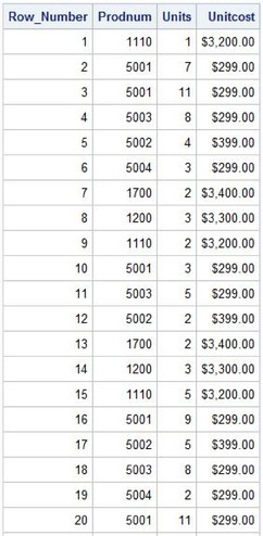
A unique undocumented, unsupported feature for producing a row (observation) count can be obtained with the MONOTONIC( ) function. Similar to the row numbers produced and displayed in output from the PRINT procedure (without the NOOBS option specified), the MONOTONIC() function displays row numbers, too. The MONOTONIC() function automatically creates a column (variable) in the output results or in a new table. Because this is an undocumented feature and is not supported in the SQL procedure, users are cautioned to use care when using the MONOTONIC() function because it is possible to obtain duplicate or missing values. The next example illustrates the creation of a row number using the MONOTONIC() function in a SELECT statement.
SQL Code
PROC SQL;
SELECT MONOTONIC() AS Row_Number FORMAT=COMMA6.,
PRODNUM,
UNITS,
UNITCOST
FROM PURCHASES;
QUIT;
Results

A row number can also be produced with the documented and supported SQL procedure option, NUMBER. Unlike the MONOTONIC() function, the NUMBER option does not create a new column in a new table. The NUMBER option is illustrated below.
SQL Code
PROC SQL NUMBER;
SELECT PRODNUM,
UNITS,
UNITCOST
FROM PURCHASES;
QUIT;
Results


The SQL procedure is a wonderful tool for summarizing (or aggregating) data. It provides a number of useful summary (or aggregate) functions to help perform calculations, descriptive statistics, and other aggregating operations in a SELECT statement or HAVING clause. These functions are designed to summarize information and not display detail about data.
Without the availability of summary functions, you would have to construct the necessary logic using somewhat complicated SQL programming constructs. When using a summary function without a GROUP BY clause, (see Chapter 3, “Formatting Output”), all the rows in a table are treated as a single group. Consequently, the results are often a single row value.
A number of summary functions are available including facilities to count non‑missing values; determine the minimum and maximum values in specific columns; return the range of values; compute the mean, standard deviation, and variance of specific values; and other aggregating functions. In the following table, an alphabetical listing of the available summary functions is displayed and, when multiple names for the same function are available, the ANSI‑approved name appears first.
|
Summary Function |
Description |
|
AVG, MEAN |
Average or mean of values |
|
COUNT, FREQ, N |
Aggregate number of non-missing values |
|
CSS |
Corrected sum of squares |
|
CV |
Coefficient of variation |
|
MAX |
Largest value |
|
MIN |
Smallest value |
|
NMISS |
Number of missing values |
|
PRT |
Probability of a greater absolute value of Student’s t |
|
RANGE |
Difference between the largest and smallest values |
|
STD |
Standard deviation |
|
STDERR |
Standard error of the mean |
|
SUM |
Sum of values |
|
SUMWGT |
Sum of the weight variable values which is 1 |
|
T |
Testing the hypothesis that the population mean is zero |
|
USS |
Uncorrected sum of squares |
|
VAR |
Variance |
The next example uses the COUNT function with the (*) argument to produce a total number of rows, whether data is missing or not. The asterisk (*) is specified as the argument to the COUNT function to count all rows in the PURCHASES table.
SQL Code
PROC SQL;
SELECT COUNT(*) AS Row_Count
FROM PURCHASES;
QUIT;
Results

Unlike the COUNT(*) function syntax that counts all rows, whether data is missing or not, the next example uses the COUNT function with the (column‑name) argument to produce a total number of non-missing rows based on the UNITS column.
SQL Code
PROC SQL;
SELECT COUNT(UNITS) AS Non_Missing_Row_Count
FROM PURCHASES;
QUIT;
Results

The MIN summary function can be specified to determine what the least expensive product is in the PRODUCTS table.
SQL Code
PROC SQL;
SELECT MIN(prodcost) AS Cheapest
Format=dollar9.2 Label=’Least Expensive’
FROM PRODUCTS;
QUIT;
Results

In the next example, the SUM function is specified to sum numeric data types for a selected column. Suppose you want to determine the total costs of all purchases by customers who bought workstations (PRODNUM=1110 and 1200) and laptops (PRODNUM=1700). You could construct the following query to sum all non-missing values for customers who purchased workstations and laptops in the PURCHASES table.
SQL Code
PROC SQL;
SELECT SUM((UNITS) * (UNITCOST))
AS Total_Purchases FORMAT=DOLLAR12.2
FROM PURCHASES
WHERE PRODNUM = 1110 OR
PRODNUM = 1200 OR
PRODNUM = 1700;
QUIT;
Results

Data can also be summarized down rows (observations) as well as across columns (variables). This flexibility gives SAS users an incredible range of power, and the ability to take advantage of several summary functions that are supplied (or built-in) by SAS. These techniques permit the average of quantities rather than the set of all quantities. Without the ability to summarize data in PROC SQL, users would be forced to write complicated formulas and/or routines, or even write and test DATA step programs to summarize data. Two examples will be illustrated to show how SQL can be constructed to summarize data:
● Summarizing data down rows
● Summarizing data across columns
Summarizing Data Down Rows
The SQL procedure can be used to produce a single aggregate value by summarizing data down rows (or observations). The advantages of using a summary function in PROC SQL is that it will generally compute the aggregate quicker than if a user-defined equation were constructed, and it saves the effort of having to construct and test a program containing the user-defined equation in the first place. Suppose you want to know the average product cost for all software in the PRODUCTS table containing a variety of products. The following query computes the average product cost and produces a single aggregate value using the AVG function.
SQL Code
PROC SQL;
SELECT AVG(PRODCOST) AS
AVERAGE_PRODUCT_COST FORMAT=DOLLAR10.2
FROM PRODUCTS
WHERE UPCASE(PRODTYPE) IN
(“SOFTWARE”);
QUIT;
Results

Summarizing Data Across Columns
When a computation is needed on two or more columns in a row, the SQL procedure can be used to summarize data across columns. Suppose you want to know the average cost of products in inventory. The next example computes the average inventory cost for each product without using a summary function, and once computed displays the value for each row as AVERAGE_PRICE.
SQL Code
PROC SQL;
SELECT PRODNUM,
(INVPRICE / INVQTY) AS
AVERAGE_PRICE
FORMAT=DOLLAR8.2
FROM INVOICE;
QUIT;
Results

Predicates are used in PROC SQL to perform direct comparisons between two conditions or expressions. Six predicates will be looked at:
● BETWEEN
● IN
● IS NULL
● IS MISSING
● LIKE
● EXISTS
Selecting a Range of Values
The BETWEEN predicate is a way of simplifying a query by selecting column values within a designated range of values. BETWEEN is equivalent to an AND combination of one LE (less than or equal) and one GE (greater than or equal) conditions; inclusive of both endpoints. It is extremely flexible because it works with character, numeric, and date values. Programmers can also combine two or more BETWEEN predicates with AND or OR operators for more complicated conditions. In the next example, a range of products costing between $200.00 and $500.00 inclusively are selected from the PRODUCTS table.
SQL Code
PROC SQL;
SELECT PRODNAME,
PRODTYPE,
PRODCOST
FROM PRODUCTS
WHERE PRODCOST BETWEEN 200 AND 500;
QUIT;
Results

In the next example, products are selected from the INVENTORY table that were ordered between the years 1999 and 2000. The YEAR function returns the year portion from a SAS date value and is used as the range of values in the WHERE clause.
SQL Code
PROC SQL;
SELECT PRODNUM,
INVENQTY,
ORDDATE
FROM INVENTORY
WHERE YEAR(ORDDATE) BETWEEN 1999 AND 2000;
QUIT;
Results

The BETWEEN predicate and OR operator are used together in the next example to select products ordered between 1999 and 2000 or where inventory quantities are greater than 15. The YEAR function returns the year portion from a SAS date value and is used as the range of values in the WHERE clause.
SQL Code
PROC SQL;
SELECT PRODNUM,
INVENQTY,
ORDDATE
FROM INVENTORY
WHERE (YEAR(ORDDATE) BETWEEN 1999 AND 2000) OR
INVENQTY > 15;
QUIT;
Results

Selecting Nonconsecutive Values
The IN predicate selects one or more rows based on the matching of one or more column values in a set of values. The IN predicate creates an OR condition between each value and returns a Boolean value of True if a column value is equal to one or more of the values in the expression list. Although the IN predicate can be specified with single column values, it may be less costly to specify the “=” sign instead. The “=” sign is used in the next example rather than the IN predicate to select phones from the PRODUCTS table.
SQL Code
PROC SQL;
SELECT PRODNAME,
PRODTYPE,
PRODCOST
FROM PRODUCTS
WHERE UPCASE(PRODTYPE) = ‘PHONE’;
QUIT;
Results

In the next example, both phones and software products are selected from the PRODUCTS table. To avoid having to specify two OR conditions, the IN predicate is specified.
SQL Code
PROC SQL;
SELECT PRODNAME,
PRODTYPE,
PRODCOST
FROM PRODUCTS
WHERE UPCASE(PRODTYPE) IN (‘PHONE’, ‘SOFTWARE’);
QUIT;
Results

Testing for NULL or MISSING Values
The IS NULL predicate is the ANSI approach of selecting one or more rows by evaluating whether a column value is missing or null (see the “Missing Values and Null section). The next example selects products from the INVENTORY table that are out-of-stock in inventory.
SQL Code
PROC SQL;
SELECT PRODNUM,
INVENQTY,
INVENCST
FROM INVENTORY
WHERE INVENQTY IS NULL;
QUIT;
SAS Log Results
PROC SQL;
SELECT PRODNUM,
INVENQTY,
INVENCST
FROM INVENTORY
WHERE INVENQTY IS NULL;
NOTE: No rows were selected.
QUIT;
NOTE: PROCEDURE SQL used:
real time 0.05 seconds
The next example selects products from the INVENTORY table that are currently stocked in inventory. Note that the predicates NOT IS NULL or IS NOT NULL can be specified to produce the same results.
SQL Code
PROC SQL;
SELECT PRODNUM,
INVENQTY,
INVENCST
FROM INVENTORY
WHERE INVENQTY IS NOT NULL;
QUIT;
Results

The IS MISSING predicate performs identically to the IS NULL predicate by selecting one or more rows containing a missing value (null). The only difference is that specifying IS NULL is the ANSI standard way of expressing the predicate and IS MISSING is commonly used in SAS. The next example uses the IS MISSING with the NOT predicate to select products from the INVENTORY table that are stocked in inventory.
SQL Code
PROC SQL;
SELECT PRODNUM,
INVENQTY,
INVENCST
FROM INVENTORY
WHERE INVENQTY IS NOT MISSING;
QUIT;
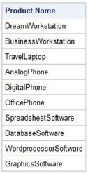
Finding Patterns in a String (Pattern Matching % and _)
Constructing specific search patterns in string expressions is a simple process with the LIKE predicate. The % (percent sign) acts as a wildcard character representing any number of characters, including any combination of upper or lower case characters. Combining the LIKE predicate with the % permits case‑sensitive searches and is a popular technique used by savvy SQL programmers to find patterns in their data.
Using the LIKE operator with the % provides a wildcard capability enabling the selection of table rows that match a specific pattern. The LIKE predicate is case‑sensitive and should be used with care. To find patterns in product name (PRODNAME) containing the uppercase character “A” in the first position followed by any number of characters is specified with the following WHERE clause.
SQL Code
PROC SQL;
SELECT PRODNAME
FROM PRODUCTS
WHERE PRODNAME LIKE ‘A%’;
QUIT;
Results

The next example illustrates the wildcard character “%” preceding and following the search word to select all products whose name contains the word “Soft” in its name. The resulting output contains product types such as “Software” and any other products containing the word “Soft”.
SQL Code
PROC SQL;
SELECT PRODNAME,
PRODTYPE,
PRODCOST
FROM PRODUCTS
WHERE PRODTYPE LIKE ‘%Soft%’;
QUIT;
Results

In the next example, the LIKE predicate is used to check a column for the existence of trailing blanks. The wildcard character % followed by a blank space is specified as the search argument.
SQL Code
PROC SQL;
SELECT PRODNAME
FROM PRODUCTS
WHERE PRODNAME LIKE ‘% ’;
QUIT;
Results
When a pattern search for a specific number of characters is needed, using the LIKE predicate with the underscore (_) provides a way to pattern match character-by-character. Thus, a single underscore (_) in a specific position acts as a wildcard placement holder for that position only. Two consecutive underscores (__) act as a wildcard placement holder for those two positions. Three consecutive underscores act as a wildcard placement holder for those three positions. And so forth. In the next example, the first position used to search product type contains the character “P”, and the next five positions (represented with five underscores) act as a placeholder for any value.
SQL Code
PROC SQL;
SELECT PRODNAME,
PRODTYPE,
PRODCOST
FROM PRODUCTS
WHERE UPCASE(PRODTYPE) LIKE ‘P_____’;
QUIT;
Results

The next example illustrates a pattern search of product name (PRODNAME) where the first three positions are represented as a wildcard; the fourth position contains the lowercase character “a”, followed by any combination of uppercase or lowercase characters.
SQL Code
PROC SQL;
SELECT PRODNAME
FROM PRODUCTS
WHERE PRODNAME LIKE ‘___a%’;
QUIT;
Results

Testing for the Existence of a Value
The EXISTS predicate is used to test for the existence of a set of values. In the next example, a subquery is used to check for the existence of customers in the CUSTOMERS table with purchases from the PURCHASES table. More details on subqueries will be presented in Chapter 7, “Coding Complex Queries.”
SQL Code
PROC SQL;
SELECT CUSTNUM,
CUSTNAME,
CUSTCITY
FROM CUSTOMERS C
WHERE EXISTS
(SELECT *
FROM PURCHASES P
WHERE C.CUSTNUM = P.CUSTNUM);
QUIT;
Results

As described earlier, the SELECT statement’s purpose is to read data from one or more tables (or data sets). In addition to selecting columns that are stored in one or more tables, SQL can be used to dynamically create new columns containing text or computations, so they exist for the duration of the query. New columns can be created in a SELECT statement by specifying a column alias with an ‘AS’ keyword. The column name must adhere to the rules for SAS names and persists for that query only. In the next example, a name is assigned to the results of a new computed column (UNITCOST * UNITS) called, TOTALCOST, using the AS keyword and is formatted with a DOLLAR10.2 format for each row in the PURCHASES table.
SQL Code
PROC SQL;
SELECT CUSTNUM
,UNITCOST
,UNITS
,UNITCOST * UNITS AS TOTALCOST FORMAT=DOLLAR10.2
FROM PURCHASES;
QUIT;
Partial Results

. . . . . .

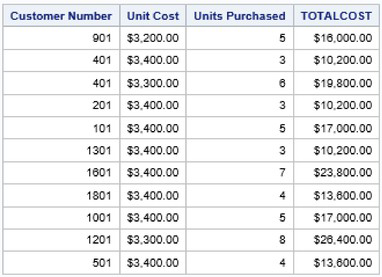
When an alias is specified to name a new column, the alias referencing the column can be used in the query. In the next example, a name and format is assigned to the results of the computed column, TOTALCOST, for each row in the PURCHASES table along with a WHERE clause to reference the computed column and to subset the results to display rows where the TOTALCOST is greater than $10,000.
SQL Code
PROC SQL;
SELECT CUSTNUM
,UNITCOST
,UNITS
,UNITCOST * UNITS AS TOTALCOST FORMAT=DOLLAR10.2
FROM PURCHASES
WHERE TOTALCOST > 10000;
QUIT;
In the previous example you learned that we can perform computations in a SELECT statement and assign an alias to any new columns that we create. So why did SAS stop processing our query in this example and send an ERROR message to the SAS log? Earlier in this chapter, we examined the order of execution of each clause in an SQL query and learned that SAS processes the WHERE clause prior to the SELECT clause. Consequently, an error is produced, as is shown below, if the computed column is used in a WHERE clause as a condition because the WHERE clause is unaware that the computed column, TOTALCOST, exists.
SAS Log Results
PROC SQL;
SELECT CUSTNUM
,UNITCOST
,UNITS
,UNITCOST * UNITS AS TOTALCOST FORMAT=DOLLAR10.2
FROM PURCHASES
WHERE TOTALCOST > 10000;
ERROR: The following columns were not found in the contributing tables: TOTALCOST.
NOTE: PROC SQL set option NOEXEC and will continue to check the syntax of statements.
QUIT;
NOTE: The SAS System stopped processing this step because of errors.
To correct the problem illustrated in the previous example, the keyword CALCULATED needs to be specified in the WHERE clause along with the alias to inform SAS that the new column is derived within the query. In the next example, a name and format is assigned to the computed column, TOTALCOST, for each row in the PURCHASES table along with a WHERE clause specifying the CALCULATED keyword followed by the alias to reference, subset and display the computed column’s results where the TOTALCOST is greater than $10,000.
SQL Code
PROC SQL;
SELECT CUSTNUM
,UNITCOST
,UNITS
,UNITCOST * UNITS AS TOTALCOST FORMAT=DOLLAR10.2
FROM PURCHASES
WHERE CALCULATED TOTALCOST > 10000;
QUIT;
Results
SAS generates and maintains valuable runtime information (metadata) about SAS libraries, data sets, catalogs, indexes, macros, system options, titles, views, and other content in a collection of read-only tables called dictionary tables. Although called tables, dictionary tables are not real tables at all. Dictionary tables and their contents permit a SAS session’s activities to be easily accessed and monitored. Information is automatically produced and each table’s contents are made available at the time a SAS session begins. Table 2.2 presents the available Dictionary tables and a description of their contents.
Table 2.2: Available Dictionary Tables and Their Contents
|
Dictionary Table Name |
Contents |
|
DICTIONARY.CATALOGS |
SAS catalogs |
|
DICTIONARY.COLUMNS |
Data set columns and attributes |
|
DICTIONARY.EXTFILES |
Allocated filerefs and external physical path |
|
DICTIONARY.INDEXES |
Data set indexes |
|
DICTIONARY.MACROS |
Global and automatic macro variables |
|
DICTIONARY.MEMBERS |
SAS data sets and other member types |
|
DICTIONARY.OPTIONS |
Current SAS system option settings |
|
DICTIONARY.TABLES |
SAS data sets and views |
|
DICTIONARY.TITLES |
Title and footnote definitions |
|
DICTIONARY.VIEWS |
SAS data views |
SAS collects and populates valuable information (“metadata” or data about data) on SAS libraries, data sets (tables), catalogs, indexes, macros, system options, titles, views, and a collection of other read-only tables called dictionary tables. Dictionary tables serve a special purpose by providing system-related information about the current SAS session’s SAS databases and applications. When a query is requested against a dictionary table, SAS automatically launches a discovery process at runtime to collect information pertinent to that table. This information is made available any time after a SAS session is started.
While SAS 9.1 has 22 dictionary tables and SASHELP views, there are 29 “known” dictionary tables and SASHELP views in SAS 9.2, 30 “known” dictionary tables and SASHELP views in SAS 9.3, and 32 “known” dictionary tables and SASHELP views in SAS 9.4. The names of each DICTIONARY table and SASHELP view are illustrated in Table 2.3 below.
Table 2.3: DICTIONARY Tables and SASHELP Views
|
DICTIONARY Table |
SASHELP View |
Purpose |
||
|
CATALOGS |
VCATALG |
Provides information about SAS catalogs. |
||
|
CHECK_CONSTRAINTS |
VCHKCON |
Provides check constraints information. |
||
|
COLUMNS |
VCOLUMN |
Provides information about column in tables. |
||
|
CONSTRAINT_COLUMN_USAGE |
VCNCOLU |
Provides column integrity constraints information. |
||
|
CONSTRAINT_TABLE_USAGE |
VCNTABU |
Provides information related to tables with integrity constraints defined. |
||
|
DATAITEMS |
VDATAIT |
Provides information about known data items. |
||
|
DESTINATIONS |
VDEST |
Provides information about known ODS destinations. |
||
|
DICTIONARIES |
VDCTNRY |
Provides information about all the DICTIONARY tables. |
||
|
ENGINES |
VENGINE |
Provides information about known SAS engines available to the session. |
||
|
EXTFILES |
VEXTFL |
Provides information related to external files. |
||
|
FILTERS |
VFILTER |
Provides information about known filters. |
||
|
FORMATS |
VFORMAT |
Provides information related to defined formats and informats. |
||
|
FUNCTIONS |
VFUNC |
Provides information about all known functions. |
||
|
GOPTIONS |
VGOPT |
Provides information about currently defined SAS/GRAPH software graphics options. |
||
|
INDEXES |
VINDEX |
Provides information related to defined indexes. |
||
|
INFOMAPS |
VINFOMP |
Provides information about all known information maps. |
||
|
LIBNAMES |
VLIBNAM |
Provides information related to defined SAS libraries. |
||
|
MACROS |
VMACRO |
Provides information related to any defined macros. |
||
|
MEMBERS |
VMEMBER |
Provides information related to objects currently defined in SAS libraries. |
||
|
OPTIONS |
VOPTION |
Provides information related to SAS system options. |
||
|
DICTIONARY Table |
SASHELP View |
Purpose |
||
|
PROMPTS |
VPROMPT |
Provides information about all known SAS/GRAPH prompts. |
||
|
PROMPTSXML |
VPRMXML |
Provides information about all known XML prompts. |
||
|
REFERENTIAL_CONSTRAINTS |
VREFCON |
Provides information related to tables with referential constraints. |
||
|
REMEMBER |
VREMEMB |
Provides information about all known remembered text. |
||
|
STYLES |
VSTYLE |
Provides information related to select ODS styles. |
||
|
TABLES |
VTABLE |
Provides information related to currently defined tables. |
||
|
TABLE_CONSTRAINTS |
VTABCON |
Provides information related to tables containing integrity constraints. |
||
|
TITLES |
VTITLE |
Provides information related to currently defined titles and footnotes. |
||
|
VIEWS |
VVIEW |
Provides information related to currently defined data views. |
||
You can view a dictionary table’s definition and enhance your understanding of each table’s contents by specifying a DESCRIBE TABLE statement. The results of the statements used to create each dictionary table can be displayed in the SAS log. For example, a DESCRIBE TABLE statement is illustrated below to display the CREATE TABLE statement used in building the OPTIONS dictionary table containing current SAS system option settings.
SQL Code
PROC SQL;
DESCRIBE TABLE
DICTIONARY.OPTIONS;
QUIT;
SAS Log Results
create table DICTIONARY.OPTIONS
(
optname char(32) label='Option Name',
setting char(1024) label='Option Setting',
optdesc char(160) label='Option Description',
level char(8) label='Option Location'
);
Note: The information contained in dictionary tables is also available to DATA and PROC steps outside the SQL procedure. Referred to as dictionary views, each view is prefaced with the letter “V” and may be shortened with abbreviated names. Dictionary view can be accessed by referencing the view by its name in the SASHELP library. See the SAS Procedures Guide for further details on accessing and using dictionary views in the SASHELP library.
To help become familiar with each dictionary table’s and dictionary view’s column names and their definitions, Tables 2.4 through 2.13 identify each unique column name, type, length, format, informat, and label.
Table 2.4: DICTIONARY.CATALOGS or SASHELP.VCATALG
|
Column |
Type |
Length |
Format |
Informat |
Label |
|
Libname |
char |
8 |
|
|
Library Name |
|
Memname |
char |
32 |
|
|
Member Name |
|
Memtype |
char |
8 |
|
|
Member Type |
|
Objname |
char |
32 |
|
|
Object Name |
|
Objtype |
char |
8 |
|
|
Object Type |
|
Objdesc |
char |
256 |
|
|
Description |
|
Created |
num |
|
DATETIME. |
DATETIME. |
Date Created |
|
Modified |
num |
|
DATETIME. |
DATETIME. |
Date Modified |
|
Alias |
char |
8 |
|
|
Object Alias |
Table 2.5: DICTIONARY.COLUMNS or SASHELP.VCOLUMN
|
Column |
Type |
Length |
Label |
|
Libname |
char |
8 |
Library Name |
|
Memname |
char |
32 |
Member Name |
|
Memtype |
char |
8 |
Member Type |
|
Name |
char |
32 |
Column Name |
|
Type |
char |
4 |
Column Type |
|
Length |
num |
|
Column Length |
|
Npos |
num |
|
Column Position |
|
Varnum |
num |
|
Column Number in Table |
|
Label |
char |
256 |
Column Label |
|
Format |
char |
16 |
Column Format |
|
Informat |
char |
16 |
Column Informat |
|
Idxusage |
char |
9 |
Column Index Type |
Table 2.6: DICTIONARY.EXTFILES or SASHELP.VEXTFL
|
Column |
Type |
Length |
Label |
|
Fileref |
char |
8 |
Fileref |
|
Xpath |
char |
1024 |
Path Name |
|
Xengine |
char |
8 |
Engine Name |
Table 2.7: DICTIONARY.INDEXES or SASHELP.VINDEX
|
Column |
Type |
Length |
Label |
|
Libname |
char |
8 |
Library Name |
|
Memname |
char |
32 |
Member Name |
|
Memtype |
char |
8 |
Member Type |
|
Name |
char |
32 |
Column Name |
|
Idxusage |
char |
9 |
Column Index Type |
|
Indxname |
char |
32 |
Index Name |
|
Indxpos |
num |
|
Position of Column in Concatenated Key |
|
Nomiss |
char |
3 |
Nomiss Option |
|
Unique |
char |
3 |
Unique Option |
Table 2.8: DICTIONARY.MACROS or SASHELP.VMACRO
|
Column |
Type |
Length |
Label |
|
Scope |
char |
9 |
Macro Scope |
|
Name |
char |
32 |
Macro Variable Name |
|
Offset |
num |
|
Offset into Macro Variable |
|
Value |
char |
200 |
Macro Variable Name |
Table 2.9: DICTIONARY.MEMBERS or SASHELP.VMEMBER
|
Column |
Type |
Length |
Label |
|
Libname |
char |
8 |
Library Name |
|
Memname |
char |
32 |
Member Name |
|
Memtype |
char |
8 |
Member Type |
|
Engine |
char |
8 |
Engine Name |
|
Index |
char |
32 |
Indexes |
|
Path |
char |
1024 |
Path Name |
Table 2.10: DICTIONARY.OPTIONS or SASHELP.VOPTION
|
Column |
Type |
Length |
Label |
|
Optname |
char |
32 |
Option Name |
|
Setting |
char |
1024 |
Option Setting |
|
Optdesc |
char |
160 |
Option Description |
|
Level |
char |
8 |
Option Location |
Table 2.11: DICTIONARY.TABLES or SASHELP.VTABLE
|
Column |
Type |
Length |
Format |
Informat |
Label |
|
Libname |
char |
8 |
|
|
Library Name |
|
Memname |
char |
32 |
|
|
Member Name |
|
Memtype |
char |
8 |
|
|
Member Type |
|
Memlabel |
char |
256 |
|
|
Dataset Label |
|
Typemem |
char |
8 |
|
|
Dataset Type |
|
Crdate |
num |
|
DATETIME. |
DATETIME. |
Date Created |
|
Modate |
num |
|
DATETIME. |
DATETIME. |
Date Modified |
|
Column |
Type |
Length |
Format |
Informat |
Label |
|
Nobs |
num |
|
|
|
# of Obs |
|
Obslen |
num |
|
|
|
Obs Length |
|
Nvar |
num |
|
|
|
# of Variables |
|
Protect |
char |
3 |
|
|
Type of Password Protection |
|
Compress |
char |
8 |
|
|
Compression Routine |
|
Encrypt |
char |
8 |
|
|
Encryption |
|
Npage |
num |
|
|
|
# of Pages |
|
Pcompress |
num |
|
|
|
% Compression |
|
Reuse |
char |
3 |
|
|
Reuse Space |
|
Bufsize |
num |
|
|
|
Bufsize |
|
Delobs |
num |
|
|
|
# of Deleted Obs |
|
Indxtype |
char |
9 |
|
|
Type of Indexes |
|
Datarep |
char |
32 |
|
|
Data Representation |
|
Reqvector |
char |
24 |
$HEX. |
$HEX. |
Requirements Vector |
Table 2.12: DICTIONARY.TITLES or SASHELP.VTITLE
|
Column |
Type |
Length |
Label |
|
Type |
char |
1 |
Title Location |
|
Number |
num |
|
Title Number |
|
Text |
char |
256 |
Title Text |
Table 2.13: DICTIONARY.VIEWS or SASHELP.VVIEW
|
Column |
Type |
Length |
Label |
|
Libname |
char |
8 |
Library Name |
|
Memname |
char |
32 |
Member Name |
|
Memtype |
char |
8 |
Member Type |
|
Engine |
char |
8 |
Engine Name |
The content of a dictionary table is accessed with the SQL procedure’s SELECT statement FROM clause. Results are displayed as rows and columns in a table, and can be used in handling common data processing tasks including obtaining a list of allocated libraries, catalogs and data sets, as well as communicating SAS environment settings to custom software applications. Users should take the time to explore the capabilities of these read-only dictionary tables and become familiar with the type of information they provide.
Dictionary.CATALOGS
Obtaining detailed information about catalogs and their members is quick and easy with the CATALOGS dictionary table. You will be able to capture an ordered list of catalog information by member name including object name and type, description, date created and last modified, and object alias from any SAS library. For example, the following code produces a listing of the catalog objects in the SASUSER library.
Note: Because this dictionary table produces a considerable amount of information, users are advised to specify a WHERE clause when using.
SQL Code
PROC SQL;
SELECT *
FROM DICTIONARY.CATALOGS
WHERE LIBNAME=”SASUSER”;
QUIT;
Results

Dictionary.COLUMNS
Retrieving information about the columns in one or more data sets is easy with the COLUMNS dictionary table. Similar to the results of the CONTENTS procedure, you will be able to capture column-level information including column name, type, length, position, label, format, informat, and indexes, as well as produce cross-reference listings containing the location of columns in a SAS library. For example, the following code requests a cross-reference listing of the tables containing the CUSTNUM column in the WORK library.
Note: Care should be used when specifying multiple functions on the WHERE clause because the SQL Optimizer is unable to optimize the query resulting in all allocated SAS session librefs being searched. This can cause the query to run much longer than expected.
SQL Code
PROC SQL;
SELECT *
FROM DICTIONARY.COLUMNS
WHERE UPCASE(LIBNAME)=”WORK” AND
UPCASE(NAME)=”CUSTNUM”;
QUIT;
Results

Dictionary.DICTIONARIES
Users can easily identify all available dictionary tables by accessing the read-only DICTIONARIES dictionary table or VDCTNRY SASHELP view. The contents of the DICTIONARIES dictionary table and VDCTNRY SASHELP view reveals the names of supported tables and views. The following PROC SQL query specifies the UNIQUE keyword to generate a listing of existing dictionary tables.
PROC SQL Code
PROC SQL;
SELECT UNIQUE MEMNAME
FROM DICTIONARY.DICTIONARIES;
QUIT;
Results

Dictionary.EXTFILES
Accessing allocated external files by fileref and corresponding physical path name information is a snap with the EXTFILES dictionary table. The results from this handy table can be used in an application to communicate whether a specific fileref has been allocated with a FILENAME statement. For example, the following code produces a listing of each individual path name by fileref.
SQL Code
PROC SQL;
SELECT *
FROM DICTIONARY.EXTFILES;
QUIT;
Results

Dictionary.INDEXES
It is sometimes useful to display the names of existing simple and composite indexes, or their SAS tables, that reference a specific column name. The INDEXES dictionary table provides important information to help identify indexes that improve a query’s performance. For example, to display indexes that reference the CUSTNUM column name in any of the example tables, the following code is specified.
Note: See Chapter 12, “Tuning for Performance and Efficiency,” for performance tuning techniques as they relate to indexes.
SQL Code
PROC SQL;
SELECT *
FROM DICTIONARY.INDEXES
WHERE UPCASE(NAME)=”CUSTNUM” /* Column Name */
AND LIBNAME=”WORK”; /* Library Name */
QUIT;
Dictionary.MACROS
The ability to capture macro variable names and their values is available with the MACROS dictionary table. The MACROS dictionary table provides information for global and automatic macro variables, but not for local macro variables. For example, to obtain columns specific to macros such as global macros SQLOBS, SQLOOPS, SQLXOBS, or SQLRC, the following code is specified.
SQL Code
PROC SQL;
SELECT *
FROM DICTIONARY.MACROS
WHERE UPCASE(SCOPE)=”GLOBAL”;
QUIT;
Results

Dictionary.MEMBERS
Accessing a detailed list of data sets, views, and catalogs is the hallmark of the MEMBERS dictionary table. You will be able to access a terrific resource of information by library, member name and type, engine, indexes, and physical path name. For example, to obtain a list of the individual files in the WORK library, the following code is specified.
SQL Code
PROC SQL;
SELECT *
FROM DICTIONARY.MEMBERS
WHERE LIBNAME=”WORK”;
QUIT;
Results

Dictionary.OPTIONS
The OPTIONS dictionary table provides a list of the current SAS session’s option settings including the option name, its setting, description, and location. Obtaining option settings is as easy as 1-2-3. Simply submit the following SQL query referencing the OPTIONS dictionary table as follows. A partial listing of the results from the OPTIONS dictionary table is displayed below in rich text format.
SQL Code
PROC SQL;
SELECT *
FROM DICTIONARY.OPTIONS;
QUIT;
Results

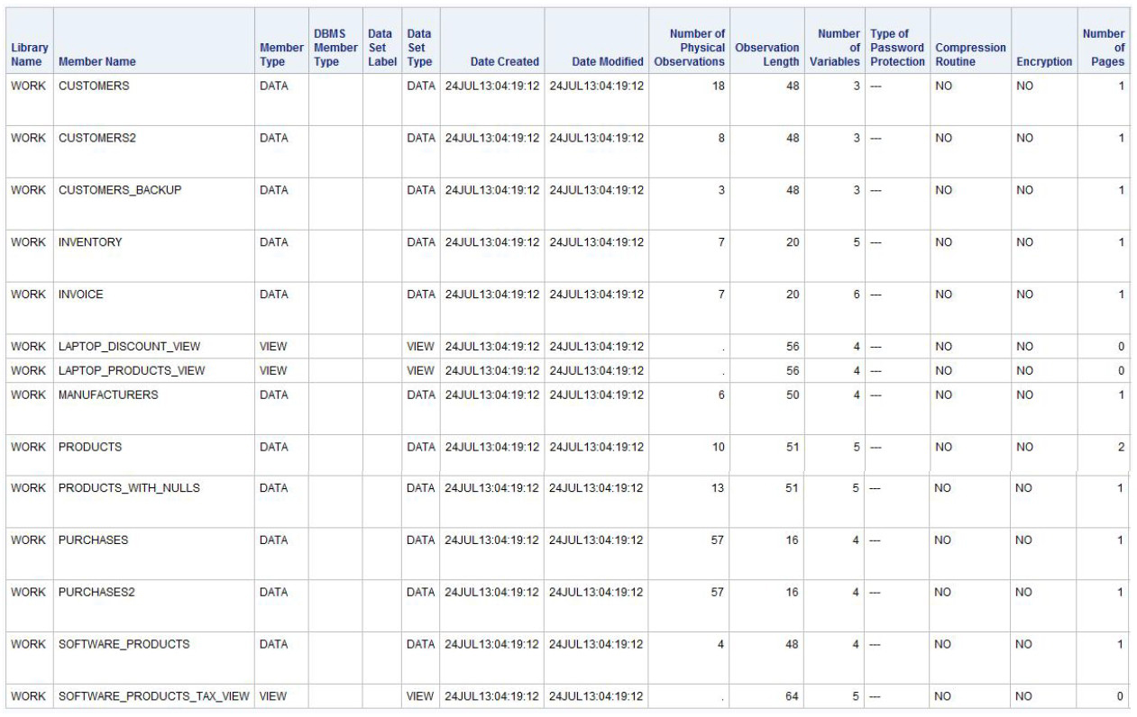
Dictionary.TABLES
When you need more information about SAS files than what the MEMBERS dictionary table provides, consider using the TABLES dictionary table. The TABLES dictionary table provides such file details as library name, member name and type, date created and last modified, number of observations, observation length, number of variables, password protection, compression, encryption, number of pages, reuse space, buffer size, number of deleted observations, type of indexes, and requirements vector. For example, to obtain a detailed list of files in the WORK library, the following code is specified.
Note: Because the TABLES dictionary table produces a considerable amount of information, users should specify a WHERE clause when using it.
SQL Code
PROC SQL;
SELECT *
FROM DICTIONARY.TABLES
WHERE LIBNAME=”WORK”;
QUIT;
Results
Dictionary.TITLES
The TITLES dictionary table provides a listing of the currently defined titles and footnotes in a session. The table output distinguishes between titles and footnotes using a “T” or “F” in the TITLE LOCATION column. For example, the following code displays a single title and two footnotes.
SQL Code
PROC SQL;
SELECT *
FROM DICTIONARY.TITLES;
QUIT;
Results

Dictionary.VIEWS
The VIEWS dictionary table provides a listing of views for selected SAS libraries. The result of the VIEWS dictionary table displays the library name, member names and type, and engine used. For example, the following code displays a single view called VIEW_CUSTOMERS from the WORK library.
SQL Code
PROC SQL;
SELECT *
FROM DICTIONARY.VIEWS
WHERE LIBNAME=”WORK”;
QUIT;
Results

Summary
1. The available data types in SQL are 1) numeric and 2) character (see the “Data Types Overview” section).
2. When a table is created with PROC SQL, numeric columns are assigned a default length of 8 bytes (see the “Numeric Data” section).
3. SAS tables store date and time information in the form of a numeric data type (see the “Date and Time Column Definitions” section).
4. A CHAR column stores a default of 8 characters (see the “Character Data” section).
5. Comparison operators are used in the SQL procedure to compare one character or numeric value to another (see the “Comparison Operators” section).
6. Logical operators are used to connect one or more expressions together in a WHERE clause and consist of AND, OR, and NOT (see the see the “Logical Operators” section).
7. The arithmetic operators used in the SQL procedure are the same as those used in the DATA step (see the “Arithmetic Operators” section).
8. Character string operators and functions are typically used with character data (see the “Character String Operators and Functions” section).
9. Predicates are used in the SQL procedure to perform direct comparisons between two conditions or expressions (see the “Predicates” section).
10. Missing or unknown information is supported by PROC SQL in a form known as a null value. A null value is not the same as a zero value (see the “Missing Values and Null” section).
11. When a new column is derived within a query, the CALCULATED keyword is specified before the column name, or alias, in a WHERE clause.
12. Dictionary tables provide information about the SAS environment (see the “Dictionary Tables” section).