
Chapter 7: Coding Complex Queries
Information Retrieval Based on Relationships
DATA Step Merges versus PROC SQL Joins
Influencing Joins with a Little Magic
Performing Computations in Joins
Joins with More Than Three Tables
Alternate Approaches to Subqueries
Passing a Single Value with a Subquery
Passing More Than One Row with a Subquery
Accessing Rows from the Intersection of Two Queries
Accessing Rows from the Combination of Two Queries
Concatenating Rows from Two Queries
Comparing Rows from Two Queries
Data Structure Transformations
Splitting a Table into Multiple Tables
One-to-One, One-to-Many, Many-to-One, and Many‑to‑Many Relationships
Processing First, Last, and Between Rows for BY‑and Groups
Determining the Number of Rows in an Input Table
Identifying Tables with the Most Indexes
In previous chapters, our discussion of queries was confined to a single table referenced with a SELECT statement. The real strength of the relational approach is the ability it gives to constructing queries that refer to several tables or even to other queries. These types of queries are referred to as complex queries. PROC SQL supports coding constructs for inner and outer joins consisting of multiple tables, implementing queries that control other queries through a process known as nesting, and combining output as a single table from multiple queries.
Let’s look at queries of a more complex nature that utilize all the features of the SQL procedure. Four complex query constructs are illustrated in this chapter.
Inner Joins
A maximum of 256 tables can be referenced in a FROM and optional WHERE clause of a SELECT statement.
Outer Joins
A maximum of two tables are referenced in a FROM and ON clause of a SELECT statement.
Subqueries
A query is embedded (nested) in the WHERE clause of a main query.
Set Operations
Results are created from two or more separate queries.
Joining two or more tables of data is a powerful feature in the relational model. The SQL procedure enables you to join tables of information quickly and easily. Linking one piece of information with another piece of information is made possible when at least one column is common to each table. A maximum of 256 tables can be combined using conventional (inner) join techniques, as opposed to a maximum of two tables at a time using outer join techniques.
This chapter discusses a number of join topics including why joins are important, the differences between the various join techniques, the importance of the WHERE clause in creating joins, creating and using table aliases, joining three or more tables of data, outer (left, right, and full) joins, subqueries, and set operations. It is important to recognize that many of these techniques can be accomplished using DATA step programming techniques, but the simplicity and flexibility found in the SQL procedure makes it especially useful, if not indispensable, as a tool for the practitioner.
As relational database systems continue to grow in popularity, the need to access normalized data stored in separate tables becomes increasingly important. By relating matching values in key columns in one table with key columns in the other table(s), you can retrieve information as if the data were stored in one huge file. The results can provide new and exciting insights into possible data relationships.
Being able to define relationships between multiple tables and retrieve information based on these relationships is a powerful feature of the relational model. A join of two or more tables provides a means of gathering and manipulating data in a single SELECT statement. You join two or more tables by specifying the table names in a SELECT statement. Joins are specified on a minimum of two tables at a time, where a column from each table is used for the purpose of connecting the two tables. Connecting columns should have “like” values and the same column attributes because the join’s success is dependent on these values.
In a typical join, you name the relevant columns in the SELECT statement, specify the tables to be joined in the FROM clause, and in the WHERE clause you specify the relationship that you want revealed. That is, you describe the data subset that you want to produce. To be of use (and of a manageable size), your join needs a WHERE clause to constrain the results and ensure their utility and relevance.
Note: When you create a join without a WHERE clause, you are creating an internal, virtual table called a Cartesian product. This table can be extremely large because it represents all possible combinations of rows and columns in the joined tables.
The purpose of this section is to briefly explain the differences (and similarities) between DATA step merges and PROC SQL joins. The reason for addressing this topic is that over the years questions have been asked about which approach is superior, inferior, faster, slower, better, worse, easier, harder, more efficient, less efficient, more demanding on a programmer’s time, less demanding on a programmer’s time, more supportable, less supportable, etc. My usual reply mentions that, “Only you and your organization will be able to answer this question completely, and here’s why.”
Besides the obvious syntax and implementation method differences with the merge using a DATA step construct and the join using a procedure supplied by SAS, both approaches achieve essentially the same results. In fact, both approaches combine two or more data sets (or tables) horizontally by matching keys, and are able to process one-to-one, one-to-many, many-to-one, and many-to-many matched combinations. Table 7.1 provides a few considerations that every SAS and SQL user should ask and answer before deciding which approach is most appropriate to use.
Table 7.1: Merge versus Join Features/Considerations
|
Features / Considerations |
DATA Step Merge |
PROC SQL Join |
|
Is there a limit to the number of data sets (or tables) that can be processed, other than disk space? |
No |
Yes (Limit of 256 tables) |
|
Is the code portable to other database implementations? |
No |
Yes |
|
Is the approach a standardized method for specifying database requests? |
No |
Yes |
|
Does a sort need to be performed for processing BY-groups? |
Yes |
No |
|
Is a common variable name required when combining data sets (or tables)? |
Yes |
No |
|
When combining data sets (or tables) is the duplicate matching column automatically overlaid? |
Yes |
No |
|
Are the results automatically printed after combining data sets (or tables)? |
No |
Yes |
The SQL procedure supports a number of complex query constructs (sometimes referred to as join types). From inner joins to left, right, and full outer joins, this chapter provides a comprehensive look at the various forms of SELECT statements that can be constructed to manipulate and transform multiple tables. The SQL procedure supports four categories of data relationships: one‑to-one, one-to-many, many-to-one, and many-to-many, where each category is classified by how the rows in each table relate to one another.
One-to-one relationships represent the simplest of join operations. It’s characterized by the tables that have a BY-group column with no repeats of BY-values (a unique BY-column) in any of the tables. It assumes that the rows of data in each table are in the exact same relative order, where the combined results will comprise row one in table one with row one in table two, row two in table one with row two in table two, row three in table one with row three in table two, and so on
One-to-many and many-to-one relationships are no more complicated than one-to-one relationships, and are easily represented by the SQL procedure. These types of relationships are characterized by one table having no repeats of BY-values and the other table having one or more repeats of BY-values.
Many-to-many relationships can be a bit more complicated than one-to-one, one-to-many, and many-to-one relationships. Many-to-many relationships are characterized by all tables having one or more repeats of by-values. There are notable advantages of using the SQL procedure to perform these types of joins. First, the column names from the source tables do not have to be identically named. Second, pre-sorting the tables is not necessary because the SQL optimizer will determine whether any indexes are available (see Chapter 6, “Modifying and Updating Tables and Indexes”) or if ordering the data is necessary using an implied ORDER BY clause.
Additional topics and examples include subqueries and set operations such as UNION, INTERSECT, and EXCEPT operators. Table 7.2 presents the various types of complex queries that are available in the SQL procedure.
Table 7.2: Types of Complex Queries
The SQL procedure contains an optimizer whose purpose is to use the best plan for query execution. A join algorithm locates, for each distinct value of the join attributes, an ordered list of elements in each relation that display that value. The SQL optimizer uses criteria to determine which join algorithm to use to optimize the query. The join construct, the structure of the data, the definition of indexes, the availability of real memory, and other factors can influence the join algorithm that is selected by the optimizer. The specific details of each of the join algorithms are described below.
Nested Loop
A nested loop join algorithm might be selected by the SQL optimizer when processing small tables of data where one table is considerably smaller than the other table, the join condition does not contain an equality condition, first row matching is optimized, or using a sort-merge or hash join has been eliminated. This algorithm operates by looping through the smaller of the tables looking for a matching key in the larger table. A nested loop join algorithm is extremely sensitive to the contents of the right table because it processes the right table for each row of the left table. For this reason, this join algorithm tends to be more CPU intensive than other choices, particularly as the table sizes increase.
Sort-Merge
A sort-merge join algorithm might be selected by the SQL optimizer when the tables are small to medium size. This algorithm operates by first sorting the tables of data (if necessary) using one or more key columns, and then, for each row in the left table, the algorithm reads all matching rows in the right table. The SQL optimizer considers using a sort-merge join algorithm when the conditions for using an index or hash join algorithm have been eliminated from consideration.
Index
An index join algorithm might be selected by the SQL optimizer when indexes created on each of the columns participating in the join relationship will improve performance. This algorithm operates by looking up each row of the smaller table by accessing the index of the larger table. The SQL optimizer considers using an index join algorithm when the larger table has an associated index with all the join keys, the tables are related with an equality condition, and/or join conditions use the AND operator between multiple expressions.
Hash
A hash join algorithm might be selected by the SQL optimizer when sufficient memory is available to the system, and the BUFFERSIZE option is large enough to store the smaller of the tables into memory. This algorithm operates by sequentially scanning the larger table and performing row-by-row lookup against the smaller table. The SQL optimizer considers using a hash join algorithm when an index join algorithm has been eliminated from consideration.
The SQL procedure supports various options to influence the execution of specific join algorithms. The following SQL procedure options are available:
Table 7.3: SQL Procedure Options
|
Option |
Description |
|
MAGIC=101 |
Influence the SQL optimizer to select the Nested Loop join algorithm. |
|
MAGIC=102 |
Influence the SQL optimizer to select the Sort-Merge join algorithm. |
|
MAGIC=103 |
Influence the SQL optimizer to select the Hash join algorithm. |
In the next example, the PROC SQL option MAGIC=101 is specified to influence the optimizer to select a nested loop join algorithm for query execution.
SQL Code
proc sql magic=101;
select c.custname,
p1.prodnum, p1.prodname, p2.units, p2.unitcost,
p2.units * p2.unitcost as Total_Cost format=dollar12.2
from products p1,
purchases p2,
customers c
where p1.prodnum = p2.prodnum AND
p2.custnum = c.custnum
order by c.custname, p1.prodname;
quit;
The log results that follow show that the SQL optimizer (or Planner) chose the nested loop (sequential loop) join algorithm when the MAGIC=101 option was specified.
SAS Log Results
proc sql magic=101;
select c.custname,
p1.prodnum, p1.prodname, p2.units, p2.unitcost,
p2.units * p2.unitcost as Total_Cost format=dollar12.2
from products p1,
purchases p2,
customers c
where p1.prodnum = p2.prodnum AND
p2.custnum = c.custnum
order by c.custname, p1.prodname;
NOTE: PROC SQL planner chooses sequential loop join.
NOTE: PROC SQL planner chooses sequential loop join.
quit;
NOTE: PROCEDURE SQL used (Total process time):
real time 0.08 seconds
cpu time 0.07 seconds
In the next example, the PROC SQL option MAGIC=102 is specified to influence the optimizer to select a sort-merge join algorithm for query execution.
SQL Code
proc sql magic=102;
select c.custname,
p1.prodnum, p1.prodname, p2.units, p2.unitcost,
p2.units * p2.unitcost as Total_Cost format=dollar12.2
from products p1,
purchases p2,
customers c
where p1.prodnum = p2.prodnum AND
p2.custnum = c.custnum
order by c.custname, p1.prodname;
quit;
The log results that follow show that the SQL optimizer (or Planner) chose the sort-merge (merge) join algorithm when the MAGIC=102 option was specified.
SAS Log Results
proc sql magic=102;
select c.custname,
p1.prodnum, p1.prodname, p2.units, p2.unitcost,
p2.units * p2.unitcost as Total_Cost format=dollar12.2
from products p1,
purchases p2,
customers c
where p1.prodnum = p2.prodnum AND
p2.custnum = c.custnum
order by c.custname, p1.prodname;
NOTE: PROC SQL planner chooses merge join.
NOTE: PROC SQL planner chooses merge join.
quit;
NOTE: PROCEDURE SQL used (Total process time):
real time 0.14 seconds
cpu time 0.09 seconds
In the next example, the PROC SQL option MAGIC=103 is specified to influence the optimizer to select a hash join algorithm for query execution.
SQL Code
proc sql magic=103;
select c.custname,
p1.prodnum, p1.prodname, p2.units, p2.unitcost,
p2.units * p2.unitcost as Total_Cost format=dollar12.2
from products p1,
purchases p2,
customers c
where p1.prodnum = p2.prodnum AND
p2.custnum = c.custnum
order by c.custname, p1.prodname;
quit;
The log results show that the SQL optimizer (or Planner) initially chose a merge join algorithm, but transformed the merge join to a hash join algorithm when the MAGIC=103 option was specified.
SAS Log Results
proc sql magic=103;
select c.custname,
p1.prodnum, p1.prodname, p2.units, p2.unitcost,
p2.units * p2.unitcost as Total_Cost format=dollar12.2
from products p1,
purchases p2,
customers c
where p1.prodnum = p2.prodnum AND
p2.custnum = c.custnum
order by c.custname, p1.prodname;
NOTE: PROC SQL planner chooses merge join.
NOTE: PROC SQL planner chooses merge join.
NOTE: A merge join has been transformed to a hash join.
NOTE: A merge join has been transformed to a hash join.
quit;
NOTE: PROCEDURE SQL used (Total process time):
real time 0.08 seconds
cpu time 0.07 seconds
As mentioned previously, the Cartesian product (or cross join) represents all possible combinations of rows and columns from the joined tables. To be exact, it represents the sum of the number of columns of the input tables plus the product of the number of rows of the input tables. Put another way, it represents each row from the first table matched with each possible row from the second table, and so on. For example, if you performed a join operation on one table that consists of 100,000 rows and on a second table that consists of 10,000 rows, you would get a Cartesian product that consists of 10 million rows.
Although the Cartesian product serves a very useful purpose in the relational model, it is essentially meaningless for a user to intentionally produce it as a final table. Besides being large, Cartesian products contain too much information and make it difficult, if not impossible, for the practitioner to select what is salient. It is only when you subset the Cartesian product by using a WHERE clause that your data becomes quantifiable and manageable. For more information on Cartesian product joins and examples that illustrate the results of these joins, go to the Author Page for this book at support.sas.com/lafler.
As mentioned previously, inner joins can handle a maximum of 256 tables at a time, and are the most recognized and widely used type of join. They are principally used to restrict rows where the specific search condition is not met. As a result, only rows that satisfy the conditions specified in the WHERE clause are kept. This is in direct contrast with outer joins (which will be discussed in a later section).
The most common form of inner join, which is often referred to as an equijoin, uses an equal sign “=” in the WHERE clause to indicate equality between the columns in two or more tables. Suppose that you want to match products with their corresponding manufacturers so that all products from each manufacturer would be listed. An equijoin is performed to equate the manufacturer number from tables PRODUCTS and MANUFACTURERS.
SQL Code
PROC SQL;
SELECT prodname, prodcost,
manufacturers.manunum, manuname
❶ ❷
FROM PRODUCTS, MANUFACTURERS
WHERE products.manunum = ❸
manufacturers.manunum;
QUIT;
❶ The PRODUCTS table is the first table specified in the FROM clause.
❷ The MANUFACTURERS table is the second table specified in the FROM clause.
❸ The specification of an equal sign “=” in a WHERE clause between the columns in the tables indicates an equality type of join.
Results
The previous example can be further qualified by adding another condition in the WHERE clause. For example, suppose that you want to display only those products from the manufacturer KPL Enterprises. The following join identifies all of the products that are manufactured by KPL Enterprises as specified in the WHERE clause (all rows that do not meet the condition of the WHERE clause are automatically excluded from the results of the join).
Note: This join assumes that you know KPL Enterprises’ unique manufacturer number.
SQL Code
PROC SQL;
SELECT prodname, prodcost,
manufacturers.manunum, manuname
FROM PRODUCTS, MANUFACTURERS
WHERE products.manunum = ❶
manufacturers.manunum AND
products.manunum = 500;
QUIT;
❶ The specification of the AND logical operator in the WHERE clause indicates that both conditions must be true in order to retrieve rows from both tables.
Results

Let’s extend our knowledge of equijoins by identifying how much money is tied up with products that are manufactured by KPL Enterprises. To accomplish this, you need to do two things. First, you need to sum the product cost (PRODCOST) column across all rows that match the WHERE clause condition. Because the objective of the equijoin is to compute a total amount for products that are manufactured by KPL Enterprises, you need to prevent duplicate rows from displaying in the results. To prevent duplicate rows, you need to specify the DISTINCT keyword.
SQL Code
PROC SQL;
SELECT DISTINCT SUM(prodcost) AS Total_Cost ❶
FORMAT=DOLLAR10.2,
manufacturers.manunum
FROM PRODUCTS, MANUFACTURERS
WHERE products.manunum =
manufacturers.manunum AND
manufacturers.manuname = ‘KPL Enterprises’;
QUIT;
❶ The DISTINCT keyword prevents duplicate rows from appearing in the result.
Results

Another type of inner join is known as a non-equijoin. As you might guess from its name, a non‑equijoin does not have an equal sign “=” specified in its WHERE clause. For example, suppose that you want to display products that are manufactured by KPL Enterprises that cost more than $299.00. The use of the greater than “>”operator gives this type of join its name.
Note: When the SQL procedure optimizer is unable to optimize a join query by reducing the Cartesian product, a message is displayed in the SAS log that indicates that the join requires performing one or more Cartesian product joins and cannot be optimized.
SQL Code
PROC SQL;
SELECT prodname, prodtype, prodcost,
manufacturers.manunum, manufacturers.manuname
FROM PRODUCTS, MANUFACTURERS
WHERE manufacturers.manunum = 500 AND
prodtype = ‘Software’ AND
prodcost > 299.00; ❶
QUIT;
❶ The specification of the greater than “>” operator in the WHERE clause indicates a non‑equijoin scenario.
SAS Log Results
PROC SQL;
SELECT prodname, prodtype, prodcost,
manufacturers.manunum, manufacturers.manuname
FROM PRODUCTS, MANUFACTURERS
WHERE manufacturers.manunum = 500 AND
prodtype = 'Software' AND
prodcost > 299.00;
NOTE: The execution of this query involves performing one or more
Cartesian product joins that cannot be optimized.
QUIT;
NOTE: PROCEDURE SQL used:
real time 0.01 seconds
cpu time 0.01 seconds
Results

The final type of inner join is referred to as a reflexive join, which is also known as a self join. As its name implies, a self join makes an internal copy of a table, and then joins the copy to itself. Essentially, a join of this type joins one copy of a table to itself for the purpose of exploiting and illustrating comparisons between table values. For example, suppose that you want to compare the prices of products side-by-side by product type with the less expensive product appearing first (as shown in the first three columns of the example results).
SQL Code
PROC SQL;
SELECT products.prodname, products.prodtype,
products.prodcost,
products_copy.prodname, products_copy.prodtype,
products_copy.prodcost
❶ ❷
FROM PRODUCTS, PRODUCTS PRODUCTS_COPY
WHERE products.prodtype = ❸
products_copy.prodtype AND
products.prodcost <
products_copy.prodcost;
QUIT;
❶ The PRODUCTS table is the primary table that is specified in the FROM clause.
❷ A copy of the PRODUCTS table called PRODUCTS_COPY is joined with the PRODUCTS table.
❸ The WHERE clause requests the same type of products to be compared side-by-side with the less expensive product appearing first.
Results

Let’s look at another example. Suppose that you want to find out the names and invoice amounts where, for each customer, you list the names and invoice amounts of each customer with larger invoice amounts. The next example illustrates a useful application of a self join.
SQL Code
PROC SQL;
SELECT invoice.custnum, invoice.invprice,
invoice_copy.custnum, invoice_copy.invprice
❶ ❷
FROM INVOICE, INVOICE INVOICE_COPY
WHERE invoice.invprice < ❸
invoice_copy.invprice;
QUIT;
❶ The INVOICE table is the primary table that is specified in the FROM clause.
❷ A copy of the INVOICE table called INVOICE_COPY is joined with the INVOICE table.
❸ The WHERE clause produces the names of customers with larger invoice amounts.
Results

Every table in a SAS library must have a unique name to reference it. Table names must conform to valid SAS naming conventions, which means that table names can have a maximum length of 32 characters and must start with a letter or underscore (see SAS Language Reference: Concepts for further details).
To minimize the number of keystrokes that are needed to reference the tables that are specified in a join query, you can assign an alias or temporary table name reference to each table. When assigned, these arbitrary aliases provide a shortcut method to the tables themselves and are in effect for the duration of the join query but no longer. In the next example, the table alias “P” is assigned to the PRODUCTS table and the alias “M” is assigned to the MANUFACTURERS table in the FROM clause. Table name references in the SELECT statement and WHERE clause are made easier as well.
SQL Code
PROC SQL;
SELECT prodnum, prodname, prodtype, M.manunum
FROM PRODUCTS P, MANUFACTURERS M ❶
WHERE P.manunum = M.manunum AND
M.manuname = ‘KPL Enterprises’;
QUIT;
❶ The assignment of the table alias “P” and the table alias “M” in the FROM clause provides a shortcut method to refer to the longer table names PRODUCTS and MANUFACTURERS.
Results

Join queries, as with simpler queries, can take full advantage of the power of the SQL procedure. Logical and arithmetic operators, predicates, and summary functions are all available for you to use. The join query is an essential component because stored information is not always available in the form that you need.
PROC SQL provides the ability to perform basic arithmetic operations such as addition, subtraction, multiplication, and division with columns that contain numeric values. Essentially, this enables any query to perform column addition, subtraction, multiplication, and division. Suppose that you want to compute the sales tax of 7.75% for all manufactured products that are sold in the state of California. In the next example, the SELECT statement shows the California sales tax (using the product cost column and the fixed sales tax percentage) computation assigns a column alias to the result column as well as a format and label to enhance the readability of the results.
SQL Code
PROC SQL;
SELECT prodname, prodtype, prodcost,
prodcost * .0775 AS SalesTax ❶
FORMAT=dollar10.2 LABEL=‘California Sales Tax’
FROM PRODUCTS P, MANUFACTURERS M
WHERE P.manunum = M.manunum AND
M.manustat = ‘CA’;
QUIT;
❶ The ability to perform basic arithmetic operations in a SELECT statement as well as assign a column alias to the result is part of the SQL ANSI standard.
Results

Up to this point, our examples have been limited to two-table joins. But what if more information is needed than the two tables can provide? To extract the required information, access to a third table might be necessary. A join with three tables is a fairly simple extension of a two-table join.
As before, each joinable column must possess the same column attributes and contain the same type of information. In addition to listing all of the required tables in the FROM clause, the WHERE clause would need to include any and all restrictions in order to subset only the rows desired. For example, suppose that you want to display only those products along with their invoice quantity that appear in the INVOICE table for the manufacturer KPL Enterprises (manunum=500).
SQL Code
PROC SQL;
SELECT P.prodname,
P.prodcost,
M.manuname,
I.invqty
FROM PRODUCTS P,
MANUFACTURERS M,
INVOICE I
WHERE P.manunum = M.manunum AND
P.prodnum = I.prodnum AND
M.manunum = 500;
QUIT;
Results

Let’s examine the construction of the WHERE clause for this three-way join a bit further. The column that contains the manufacturer number from the PRODUCTS, MANUFACTURERS, and INVOICE tables is joined by using an AND logical operator in the WHERE clause. Additionally, the WHERE clause restricts the resulting table to only product invoices for manufacturer (manunum=500). In the next example, a three-way join lists the product names and costs, along with the customer who bought each product.
SQL Code
PROC SQL;
SELECT P.prodname,
P.prodcost,
C.custname,
I.invprice
FROM PRODUCTS P,
INVOICE I,
CUSTOMERS C
WHERE P.prodnum = I.prodnum AND
I.custnum = C.custnum;
QUIT;
Results

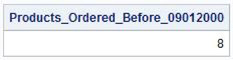
Occasionally, information needs to be extracted from four, five, or more tables (up to a maximum of 256 tables). Joins of four or more tables can be constructed just like those accessing two or three tables. The only difference is the number of table references in the FROM clause and the level of complexity in the WHERE clause to restrict what rows are kept. Suppose that you want to know, based on invoices, the number of products that were ordered before September 1, 2000. One way to find this information is to perform a join with four tables.
SQL Code
PROC SQL;
SELECT sum(inventory.invenqty)
AS Products_Ordered_Before_09012000
FROM PRODUCTS,
INVOICE,
CUSTOMERS,
INVENTORY
WHERE inventory.orddate < mdy(09,01,00) AND
products.prodnum = invoice.prodnum AND
invoice.custnum = customers.custnum AND
invoice.prodnum = inventory.prodnum;
QUIT;
Results
If you were wondering whether this result could have been derived another way, you would be correct. You could also determine, based on invoices, the number of products that were ordered before September 1, 2000, with the following two-way join code. As with this example, there is often more than one way to construct a join to extract the information that you want.
SQL Code
PROC SQL;
SELECT sum(inventory.invenqty)
AS Products_Ordered_Before_09012000
FROM INVOICE I,
INVENTORY I2
WHERE inventory.orddate < mdy(09,01,00) AND
invoice.prodnum = inventory.prodnum;
QUIT;
Results

To expand your understanding of joins with more than three tables, the following example illustrates a four-table join. Suppose that you want to know which products are being purchased and who is purchasing them. The next example shows a four-way inner join that combines data from the MANUFACTURERS, PRODUCTS, INVOICE, and CUSTOMERS tables.
SQL Code
PROC SQL;
SELECT products.prodname,
products.prodtype,
customers.custname,
manufacturers.manuname
FROM MANUFACTURERS,
PRODUCTS,
INVOICE,
CUSTOMERS
WHERE manufacturers.manunum = products.manunum AND
manufacturers.manunum = invoice.manunum AND
products.prodnum = invoice.prodnum AND
invoice.custnum = customers.custnum;
QUIT;
Results

As the previous examples in this chapter have shown, an inner join disregards any rows where the search condition is not met. This differs significantly from the way an outer join groups tables. In contrast with an inner join, an outer join keeps rows that match the ON (search) condition, as well as preserving some or all of the unmatched data from one or both of the tables. Essentially, an outer join retains rows from one table even when they do not match rows in the second table. This distinction is critical because this is what truly differentiates an outer join from an inner join.
Next, an outer join is capable of processing a maximum of two tables at a time, whereas (under the SAS implementation) an inner join is able to process a maximum of 256 tables.
Another difference has to do with how you specify outer join syntax. The comma that is used to designate or delimit one table from the other table in the FROM clause of inner joins is replaced with one of the following keywords: LEFT JOIN, RIGHT JOIN, or FULL JOIN in outer joins. Additionally, the WHERE clause expression that is used to restrict what rows are kept in the result table is replaced with the ON keyword.
Finally, an outer join is considered to be an asymmetric join (Lorie and Daudenarde, 1991, 87). Unlike inner joins, an outer join does not select rows proportionally from its parts or tables.
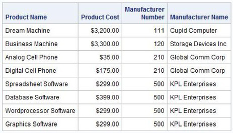
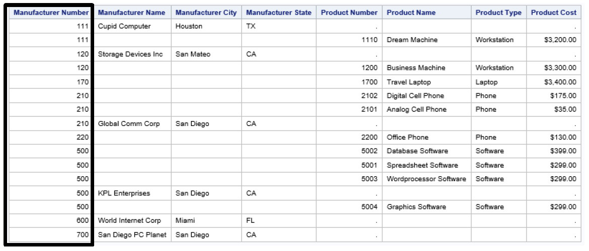
Let’s look at how a left join is applied in a real-world situation. Suppose that you want to see a list of all manufacturers, their city locations, their manufacturer numbers, their product types, and their product costs (if available) without leaving out those manufacturers that do not have products yet. This means that the MANUFACTURERS table (left table) acts as the master table having its rows preserved while the PRODUCTS table (right table) acts as the contributing table (subordinate table). The following left outer join example effectively retains those matched rows from both tables as well as retaining those rows from the left table that have no match in the right table.
SQL Code
PROC SQL;
SELECT manuname, manucity, manufacturers.manunum,
products.prodtype, products.prodcost
FROM MANUFACTURERS LEFT JOIN PRODUCTS ❶
ON manufacturers.manunum = ❷
products.manunum;
QUIT;
❶ The LEFT JOIN specification preserves all of the rows in the left table (MANUFACTURERS) even when there are no matching rows in the right table (PRODUCTS).
❷ The ON clause acts as a WHERE clause to select the desired rows in the join results.
As the results from the left outer join illustrate, the rows in the left (MANUFACTURERS) table that match rows in the right (PRODUCTS) table are included in the result table. As a result, eight rows match as evidenced by the value assigned to product type and product cost. Additionally, two rows from the left table that do not match rows in the right table (based on the search condition) are also retained (bolded). Therefore, each row from the MANUFACTURERS table that does not have a matching value in the PRODUCTS table is added to the resulting virtual table, accompanied by null values in the product type and product cost columns.
Results

Specifying a WHERE Clause
To provide greater subsetting capabilities as well as added flexibility, the SQL procedure also permits the specification of an optional WHERE clause in addition to an ON clause when constructing outer joins. The ability to specify a WHERE clause in conjunction with an ON clause permits greater control over the subsetting of rows. An example will help illustrate how a WHERE clause is used in an outer join. Suppose that you want to limit the results from the previous left outer join to only those products that cost less than $300.00. In this example, the left outer join syntax uses a WHERE clause to subset row results to nonmissing products that cost less than $300.00.
SQL Code
PROC SQL;
SELECT manuname, manucity, manufacturers.manunum,
products.prodtype, products.prodcost
FROM MANUFACTURERS LEFT JOIN PRODUCTS
ON manufacturers.manunum =
products.manunum
WHERE prodcost < 300 AND ❶
prodcost NE .;
QUIT;
❶ The optional WHERE clause that is specified in addition to an ON clause in an outer join further subsets the joined results.
Results

Specifying Aggregate Functions
Suppose that you need to produce a monthly report that consists of a total invoice amount by manufacturer. An aggregate function can be specified with outer join syntax to perform a group computation using a GROUP BY clause. In the next example, a left join computes the total invoice amount for each manufacturer with a SUM function and GROUP BY clause.
SQL Code
PROC SQL;
SELECT manuname,
SUM(invoice.invprice) AS Total_Invoice_Amt ❶
FORMAT=DOLLAR10.2
FROM MANUFACTURERS LEFT JOIN INVOICE
ON manufacturers.manunum =
invoice.manunum
GROUP BY MANUNAME; ❷
QUIT;
❶ The SUM function computes the total invoice amount for each manufacturer.
❷ The GROUP BY clause groups all of the rows associated with a manufacturer into a single row.
The results show that manufacturers with no activity have a null or missing value in the aggregated Total_Invoice_Amt column.
Results

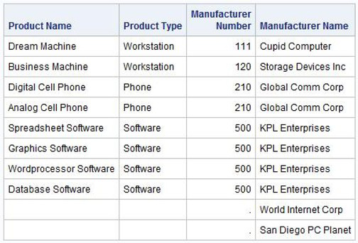
Right joins are similar to left joins, except that the rows in the right (second) table are preserved. Consequently, the results contain the rows of the symmetric join plus a row for each unmatched row in the right table. Nulls are automatically substituted for values from the left table. Suppose that you want to see all manufacturers and their respective products. In the next example, a simple report that contains products, product type, manufacturer number, and manufacturer name is produced from the PRODUCTS and MANUFACTURERS tables using a right outer join construct.
SQL Code
PROC SQL;
SELECT prodname, prodtype,
products.manunum, manuname
FROM PRODUCTS RIGHT JOIN MANUFACTURERS ❶
ON products.manunum =
manufacturers.manunum;
QUIT;
❶ The RIGHT JOIN specification preserves all of the rows in the right table (MANUFACTURERS) even when there are no matching rows in the left table (PRODUCTS).
The results show that manufacturers that appear in the MANUFACTURERS table with no products listed in the PRODUCTS table have null or missing values in the Product Name, Product Type, and Manufacturer Number columns.
Note: To remove rows with missing values in the results, a WHERE clause could be specified.
Results
Full outer joins combine the power of left and right joins by preserving rows from both the left and right tables. Although a full join is not used as frequently as left join or right join constructs, it can be useful when information from both tables is missing. In the next example, a full outer join is specified to produce a report that contains manufacturers with no products and products with no known manufacturers.
SQL Code
PROC SQL;
SELECT prodname, prodtype,
products.manunum, manuname
FROM PRODUCTS FULL JOIN MANUFACTURERS ❶
ON products.manunum =
manufacturers.manunum;
QUIT;
❶ The full join specification preserves all of the rows in the left table (PRODUCTS) as well as all of the rows in the right table (MANUFACTURERS) even when there are no matching rows.
Results

Now that you have seen how two or more tables can be combined in a join query, turn your attention to another type of complex query known as a subquery. A subquery is a query expression that is nested within another query expression. Its purpose is to have the inner query produce a single value or multiple values that can then be passed into the outer query for processing. You achieve this by embedding a SELECT statement inside a WHERE clause of an outer query’s SELECT statement, INSERT statement, DELETE statement, or HAVING clause.
Note: You should avoid nesting more than two subqueries deep because of the conceptual and processing complexities this introduces.
The typical subquery consists of a (inner) query combined inside the predicate of another (outer or main) query. When processed, the inner query passes a Boolean value to the outer query consisting of either True if it returns a minimum of one row or False if no rows are returned by the subquery. The results of the inner query are stored in a temporary results table and used as input to the main query. Our exploration of subqueries will involve using them with comparison operators, the IN predicate, and the ANY and ALL keywords, and will conclude with a look at a special type of subquery called a correlated subquery.
A subquery is a very useful construct, especially when information from multiple tables needs to be interrelated. Unfortunately, a subquery is not always easy to construct and might be even more difficult to understand. So before constructing every table relation with a subquery, consider your options carefully.
When all of the information is available in a single table, a simple query is probably all that needs to be constructed. Suppose that you want to produce a report that consists of the invoice information for Global Comm Corp. Let’s further assume that you know the specific manufacturer number for Global Comm Corp. Knowing this means that you don’t have to go into the MANUFACTURERS table to find it. In the next example, a simple query is constructed to retrieve all of the invoice information from the INVOICE table.
Simple Query
PROC SQL;
SELECT *
FROM INVOICE
WHERE manunum = 210;
QUIT;
Results

But, what if all the information is not in a single table? And what if the manufacturer number for Global Comm Corp is not known? As shown previously, a join can be constructed just as easily as a subquery. Some users prefer joins to subqueries because joins can be easier to understand and maintain. In fact, a join frequently performs better than a subquery. In the next example, the manufacturer number for Global Comm Corp is not known. Consequently, a simple inner join is needed to retrieve all related rows from the MANUFACTURERS and INVOICE tables for Global Comm Corp.
Simple Join
PROC SQL;
SELECT M.manunum, M.manuname, I.invnum,
I.invqty, I.invprice
FROM MANUFACTURERS M, INVOICE I
WHERE M.manunum = I.manunum AND
M.manuname = ‘Global Comm Corp’;
QUIT;
Results

Let’s see how a subquery could be constructed to provide the same results as with the join. As before, suppose that you want to pull all of the invoices for the manufacturer Global Comm Corp but know only the manufacturer name (or at least part of the name), but not the manufacturer number (MANUNUM). The following subquery uses an = (equal sign) in its outer query WHERE clause to accomplish this.
Because the manufacturer number is not known, a subquery is constructed to first search for the manufacturer number in the MANUFACTURERS table. Actually, the subquery approach is more versatile than the previous query approach, because it does not require a unique manufacturer number, which is often more difficult to remember than a manufacturer names. It also enables quick searches even if the manufacturer number changes for a given manufacturer.
When the entire query is executed, SQL first evaluates the inner query (or subquery) within the outer query’s WHERE clause. It executes the inner query the same way as if it were a standalone query. It searches the MANUFACTURERS table for any row where the manufacturer name equals the character string Global Comm Corp, and then pulls the MANUNUM values for this row. SQL then substitutes the derived MANUNUM value of 210 from the inner query inside the predicate of the main query (outer query). As a result of this substitution, the SQL query looks identical to the query mentioned previously.
SQL Code
PROC SQL FEEDBACK;
SELECT invnum, INVOICE.manunum, custnum, invqty, invprice, prodnum
FROM INVOICE,
(SELECT manunum ❶
FROM MANUFACTURERS
WHERE manuname = 'Global Comm Corp')
WHERE INVOICE.manunum = MANUFACTURERS.manunum;
QUIT;
Result of Inner Query
PROC SQL;
SELECT *
FROM INVOICE
WHERE manunum = 210; ❷
QUIT;
❶ PROC SQL evaluates the inner query within the outer query’s WHERE clause to search for the manufacturer number for manufacturer Global Comm Corp.
❷ The resulting query after substituting the derived manufacturer number value from the inner query evaluates to a single value, and is then executed as the main (outer) query.
Results

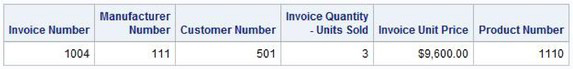
Let’s look at another subquery. Suppose that you want to retrieve the invoice from the INVOICE table for the manufacturer that manufactures the Dream Machine workstation. The following subquery (inner query) extracts the product number (PRODNUM) that is associated with the Dream Machine, and passes the single value to the outer query for processing.
SQL Code
PROC SQL FEEDBACK;
SELECT invnum, manunum, custnum, invqty, invprice,
INVOICE.prodnum
FROM INVOICE
(SELECT prodnum ❶
FROM PRODUCTS
WHERE prodname LIKE 'Dream%');
QUIT;
Result of Inner Query
PROC SQL;
SELECT *
FROM INVOICE
WHERE prodnum = 1110; ❷
QUIT;
❶ PROC SQL evaluates the inner query within the outer query’s WHERE clause to search for the product number for the Dream Machine product.
❷ The resulting inner query after substituting the derived product number value evaluates to a single value, and is then executed as the main (outer) query.
Results
It is fortunate that the subquery in the previous example passed only one row or value to the main (outer) query. Had it returned more than one value from the PRODUCTS table, it would have made it impossible for the SQL procedure to evaluate the condition as true or false and would have produced an error in the outer query. Let’s look at another example where more than one value is returned by the subquery.
In the next example, more than one row is returned by the inner query making it impossible for the main query to evaluate as true or false. As a result, an error is produced and the subquery does not execute. In general, it is best to avoid using the = (equal sign) and other comparison operators (<, >, <=, >=, and <>) in a subquery expression unless you know in advance that the result of the subquery is a table with a single row of data (although it might not always be possible to know this beforehand). In the “Passing More Than One Row with a Subquery”) section in this chapter, you will see this problem alleviated by using the IN predicate.
SQL Code
PROC SQL;
SELECT *
FROM INVOICE
WHERE manunum =
(SELECT manunum
FROM MANUFACTURERS
WHERE UPCASE(manucity) LIKE 'SAN DIEGO%');
QUIT;
SAS Log Result
PROC SQL;
SELECT *
FROM INVOICE
WHERE manunum =
(SELECT manunum
FROM MANUFACTURERS
WHERE UPCASE(manucity) LIKE 'SAN DIEGO%');
ERROR: Subquery evaluated to more than one row.
QUIT;
NOTE: The SAS System stopped processing this step because of errors.
NOTE: PROCEDURE SQL used:
real time 0.00 seconds
Let’s look at another subquery example that uses the comparison operator < (less than). A summary function specified in an inner query forces a single row to result. In the next example, the subquery uses the AVG summary (aggregate) function to determine which products (based on their invoice quantities) were purchased in lower quantities than the average product purchase.
SQL Code
PROC SQL;
SELECT prodnum, invnum, invqty, invprice
FROM INVOICE
WHERE invqty <
(SELECT AVG(invqty) ❶
FROM INVOICE);
QUIT;
Result of Inner Query
PROC SQL;
SELECT prodnum, invnum, invqty, invprice
FROM INVOICE
WHERE invqty < 4.285714; ❷
QUIT;
❶ PROC SQL evaluates the inner query within the outer query’s WHERE clause to produce an average invoice quantity.
❷ The resulting inner query passes the derived average invoice quantity of 4.285714 as a single value to the main (outer) query for execution.
Results

PROC SQL does not permit a subquery to select more than one column. To prevent this problem, which is associated with passing more than one value to the main (outer) query, you can specify the IN predicate in a subquery. Similar to the IN operator in the DATA step, the IN predicate permits the SQL procedure to pass multiple row values from the (inner) subquery to the main (outer) query without producing an error.
The next example shows how multiple row values are passed from the subquery to the main (outer) query using the IN predicate for San Diego manufacturers.
SQL Code
PROC SQL;
SELECT *
FROM INVOICE
WHERE manunum IN ❶
(SELECT manunum
FROM MANUFACTURERS
WHERE UPCASE(manucity) LIKE 'SAN DIEGO%'); ❷
QUIT;
Result of Inner Query
PROC SQL;
SELECT prodnum, invnum, invqty, invprice
FROM INVOICE
WHERE manunum IN (210, 500, 700); ❸
QUIT;
❶ PROC SQL’s IN predicate is specified in the outer query to process a list of values that are passed from the inner query.
❷ PROC SQL evaluates the inner query within the outer query’s WHERE clause to produce a list of manufacturer numbers for San Diego manufacturers.
❸ The resulting inner query passes multiple row values to the main (outer) query for execution.
Results

A subquery can have multiple values returned for a single column to the outer query. But there are special keywords that permit comparison operators to be used in subqueries to process multiple values. The special keywords ANY and ALL can be used to compare a set of values returned by a subquery. Let’s see how these keywords work.
Suppose that you want to view the products whose inventory quantity is greater than or equal to the lowest average inventory quantity. The following example illustrates a subquery with the ANY keyword specified in the WHERE clause of the main query expression. When ANY is specified, the entire WHERE clause is true if the subquery returns at least one value.
SQL Code
PROC SQL;
SELECT manunum, prodnum, invqty, invprice
FROM INVOICE
WHERE invprice GE ANY ❶
(SELECT invprice
FROM INVOICE
WHERE prodnum IN (5001,5002)); ❷
QUIT;
Result of Inner Query
PROC SQL;
SELECT manunum, prodnum, invqty, invprice
FROM INVOICE
WHERE invprice > ANY ($1,495.,$798.); ❸
QUIT;
❶ PROC SQL retrieves any invoices from the outer query where the invoice price is greater than or equal to the row values that are passed from the inner query.
❷ The WHERE clause of the inner query retrieves any invoice prices for product numbers 5001 and 5002 and passes them to the outer query.
❸ The resulting inner query passes multiple row values to the main (outer) query for execution.
Results

The ALL keyword works very differently from the ANY keyword. When you specify ALL before a subquery expression, the subquery is true only if the comparison is true for values that are returned by the subquery. For example, suppose that you want to view the products whose inventory quantity is less than the average inventory quantity?
SQL Code
PROC SQL;
SELECT manunum, prodnum, invqty, invprice
FROM INVOICE
WHERE invprice < ALL ❶
(SELECT invprice
FROM INVOICE
WHERE prodnum IN (5001,5002)); ❷
QUIT;
Result of Inner Query
PROC SQL;
SELECT manunum, prodnum, invqty, invprice
FROM INVOICE
WHERE invprice < ALL ($1,495.,$798.); ❸
QUIT;
❶ PROC SQL retrieves all invoices from the outer query where the invoice price is less than the row values that are passed from the inner query.
❷ The WHERE clause of the inner query retrieves all invoice prices for product numbers 5001 and 5002 and passes them to the outer query.
❸ The resulting inner query passes multiple row values to the main (outer) query for execution.
Results

In the subquery examples shown previously, the subquery (inner query) operates independently from the main (outer) query. Essentially, the subquery’s results are evaluated and used as input to the main (outer) query. Although this is a common way that subqueries execute, it is not the only way. SQL also permits a subquery to accept one or more values from its outer query. Once the subquery executes, the results are then passed to the outer query. Subqueries of this variety are called correlated subqueries. The ability to construct subqueries in this manner provides a powerful extension to SQL.
The difference between the subqueries discussed previously and correlated subqueries is in the way the WHERE clause is constructed. Correlated subqueries relate a column in the subquery with a column in the outer query to determine the rows that match or in certain cases don’t match the expression. Suppose, for example, that you want to view products in the PRODUCTS table that do not appear in the INVOICE table. One way to do this is to construct a correlated subquery.
In the next example, the subquery compares the product number column in the PRODUCTS table with the product number column in the INVOICE table. If at least one match is found (the product appears in both the PRODUCTS and INVOICE tables), then the resulting table from the subquery will not be empty, and the NOT EXISTS condition will be false. However, if no matches are found, then the subquery returns an empty table that results in the NOT EXISTS condition being true, which causes the product number, product name, and product type of the current row in the main (outer) query to be selected.
SQL Code
PROC SQL;
SELECT prodnum, prodname, prodtype
FROM PRODUCTS
WHERE NOT EXISTS ❶
(SELECT *
FROM INVOICE
WHERE PRODUCTS.prodnum = INVOICE.prodnum); ❷
QUIT;
❶ The (inner) subquery receives its value(s) from the main (outer) query. With the value(s), the subquery runs and passes the results back to the main query where the WHERE clause and the NOT EXISTS condition are processed.
❷ The inner query selects matching product and invoice information and passes it to the outer query.
Results

Correlated subqueries are useful for placing restrictions on the results of an entire query with a HAVING clause (or, when combined with a GROUP BY clause, of an entire group). Suppose that you want to know which manufacturers have more than one invoiced product.
In the next example, the subquery compares the manufacturer number in the PRODUCTS table with the manufacturer number in the INVOICE table. A HAVING clause and a COUNT function are specified to select all manufacturers with two or more invoices. Because an aggregate (summary) function is used in an optional HAVING clause, a GROUP BY clause is not needed to select the manufacturers with two or more invoices. An EXISTS condition is specified in the outer query’s WHERE clause to capture only those manufacturers that match the subquery.
SQL Code
PROC SQL;
SELECT prodnum, prodname, prodtype
FROM PRODUCTS
WHERE EXISTS ❶
(SELECT *
FROM INVOICE
WHERE PRODUCTS.manunum = INVOICE.manunum
HAVING COUNT(*) > 1); ❷
QUIT;
❶ The (inner) subquery receives its value(s) from the main (outer) query. With the value(s), the subquery runs and passes the results back to the main query where the WHERE clause and the EXISTS condition are processed.
❷ The inner query specifies a HAVING clause in order to subset manufacturers with two or more invoices.
Results

Now that you have seen how tables are combined with join queries and subqueries, let’s look at another type of complex query. The SQL procedure provides users with several table operators: INTERSECT, UNION, OUTER UNION, and EXCEPT, which are commonly referred to as set operators. In contrast to joins and subqueries where query results are combined horizontally, the purpose of each set operator is to combine or concatenate query results vertically. Essentially, set operators construct compound queries by combining the result sets of two or more queries.
Set operators adhere to basic rules of operation.
1. If a SELECT statement consists of more than one set operator, set operators will be applied in the order specified.
2. By default, duplicate rows are eliminated from the results.
3. To allow duplicates, the ALL option must be specified with a set operator.
4. Arguments are evaluated from left to right.
5. Set operators can be used in
a. Queries
b. Subqueries
c. Derived tables
d. View definitions
e. INSERT with SELECT clause
Set operators adhere to an order of precedence. The following precedence rules apply:
1. When more than one set operator is specified, each is applied in the order specified:
a. Top to bottom
b. to right
2. The default order of precedence for processing set operators follows:
a. INTERSECT
b. UNION and/or EXCEPT
c. When parentheses are specified, the default order of precedence can be altered.
The INTERSECT operator creates query results that consist of all the unique rows from the intersection of the two queries. Put another way, the intersection of two queries (A and B) is represented by C, which indicates that the rows that are produced occur in both A and in B. As Figure 7.1 shows, the intersection of both queries is represented in the shaded area (C).
Figure 7.1: Intersection of Two Queries

To see all products that cost less than $300.00 and product types classified as “phone”, you could construct a simple query with a WHERE clause or specify the intersection of two separate queries. The next example illustrates a simple query that specifies a WHERE clause to display phones that cost less than $300.00.
SQL Code
PROC SQL;
SELECT *
FROM PRODUCTS
WHERE prodcost < 300.00 AND
prodtype = ‘Phone’;
QUIT;
Results

The INTERSECT approach can be constructed to produce the same results as in the previous example. The INTERSECT process assumes that the tables in each query are structurally identical to each other. It overlays the columns from both queries based on position in the SELECT statement. Should you attempt to intersect two queries with different table structures, the process might fail due to differing column types, or the results might contain data integrity issues.
The most significant distinction between the two approaches, and one that might affect large table processing, is that the first query example (using the AND operator) takes less time to process: 0.05 seconds versus 0.17 seconds for the second approach (using the INTERSECT operator). The next example shows how the INTERSECT operator achieves the same result less efficiently.
SQL Code
PROC SQL;
SELECT * ❶
FROM PRODUCTS
WHERE prodcost < 300.00
INTERSECT ❷
SELECT * ❶
FROM PRODUCTS
WHERE prodtype = “Phone”;
QUIT;
❶ It is assumed that the tables in both queries are structurally identical because the wildcard character “*” is specified in the SELECT statement.
❷ The INTERSECT operator produces rows that are common to both queries.
Results

The UNION operator preserves all of the unique rows from the combination of queries. The result is the same as if an OR operator is used to combine the results of each query. Put another way, the union of two queries (A and B) represents rows in A or in B or in both A and B. As illustrated in Figure 7.2, the union represents the entire shaded area (A, B, and C).
Figure 7.2: Union of Two Queries

The UNION operator automatically eliminates duplicate rows from the results, unless the ALL keyword is specified as part of the UNION operator. The column names assigned to the results are derived from the names in the first query.
In order for the union of two or more queries to be successful, each query must specify the same number of columns of the same or compatible types. Type compatibility means that column attributes are defined the same way. Because column names and attributes are derived from the first table, data types must be of the same type. The data types of the result columns are derived from the source table(s).
To see all products that cost less than $300.00 or products that are classified as a workstation, you have a choice between using OR as shown in the following query or UNION as shown in the next query. As illustrated in the output from both queries, the results are identical no matter which query is used.
SQL Code
PROC SQL;
SELECT *
FROM PRODUCTS
WHERE prodcost < 300.00 OR
prodtype = “Workstation”;
QUIT;
Results

In the next example, the UNION operator is specified to combine the results of both queries.
SQL Code
PROC SQL;
SELECT *
FROM PRODUCTS
WHERE prodcost < 300.00
UNION ❶
SELECT *
FROM PRODUCTS
WHERE prodtype = ‘Workstation’;
QUIT;
❶ The UNION operator combines the results of two queries.
Results

The OUTER UNION operator concatenates the results of two queries. As with a DATA step or PROC APPEND concatenation, the results consist of rows that are combined vertically. Put another way, the outer union of two queries (A and B) represents all rows in both A and B with no overlap. As illustrated in Figure 7.3, the outer union represents the entire shaded area (A and B).
Figure 7.3: Outer Union of Two Queries

The next example concatenates the results of two queries. As illustrated in the results, the rows from both queries are concatenated.
SQL Code
PROC SQL;
SELECT prodnum, prodname, prodtype, prodcost
FROM PRODUCTS
OUTER UNION ❶
SELECT prodnum, prodname, prodtype, prodcost
FROM PRODUCTS;
QUIT;
❶ The OUTER UNION operator concatenates the results of both queries.
Results

The OUTER UNION operator automatically concatenates rows from two queries with no overlap, unless the CORRESPONDING (CORR) keyword is specified as part of the operator. The column names that are assigned to the results are derived from the names in the first query. In the next example, the CORR keyword enables columns with the same name and attributes to be overlaid.
SQL Code
PROC SQL;
SELECT prodnum, prodname, prodtype, prodcost
FROM PRODUCTS
OUTER UNION CORR ❶
SELECT prodnum, prodname, prodtype, prodcost
FROM PRODUCTS;
QUIT;
❶ The OUTER UNION operator with the CORR keyword concatenates and overlays the results of both queries.
Results

The EXCEPT operator compares rows from two queries to determine the changes made to the first table that are not present in the second table. The following results show new and changed rows in the first table that are not in the second table, but do not show rows that have been deleted from the second table. As illustrated in Figure 7.4, the results of specifying the EXCEPT operator represent the shaded area (A).
Figure 7.4: Compare Two Tables to Determine Additions and Changes

When working with two tables that consist of similar information, you can use the EXCEPT operator to determine new and modified rows. The EXCEPT operator is used to identify rows in the first table (or query), but is not used to identify rows in the second table (or query). It also uniquely identifies rows that have changed from the first table to the second table. Columns are compared in the order that they appear in the SELECT statement.
If the wildcard character “*” is specified in the SELECT statement, it is assumed that the tables are structurally identical to one another. Let’s look at an example.
Suppose that you have master and backup tables of the CUSTOMERS file, and you want to compare them to identify the new and changed rows. The EXCEPT operator as illustrated in the next example returns all new or changed rows from the CUSTOMERS table that do not appear in the CUSTOMERS_BACKUP table. As illustrated in the results, three new customer rows are added to the CUSTOMERS table that had not previously existed in the CUSTOMERS_BACKUP table.
SQL Code
PROC SQL;
SELECT *
FROM CUSTOMERS_BACKUP
EXCEPT ❶
SELECT *
FROM CUSTOMERS;
QUIT;
❶ The EXCEPT operator compares rows in both tables to identify the rows existing in the first table but not the second table.
Results

Data structure transformations involve the process of taking a table’s observations and/or columns of data in one format and converting them to another format. This is a common step that many, if not most, users need to perform when extracting, transforming, and loading (ETL) data in preparation for conducting data analysis. It’s also a common practice that organizations implement one or more business rules to safeguard the data transformation process from data accuracy and integrity from occurring. For example, a business rule might be implemented to prevent products from being purchased by customers when a product is never actually sold by a manufacturer. Should a business rule like this be violated then a WTF (Where’s This From) error handling routine would be triggered to help alert the organization of the situation.
The big question on many users’ minds is why anyone should care about transforming data structures. The simple answer is in many database environments data is not always stored in the way it’s needed for conducting analysis. In fact, it’s frequently found that data in one database table is not stored in the same way as it is in another table. Due to the propensity of inconsistent data mappings of key (or other important) data values, users are frequently faced with finding ways to prep and transform data structures to a desired format for analysis purposes.
There are many types of data structure transformations that users should be familiar with. The following table illustrates the leading types of data structure transformations along with a brief description of each.
|
Transformation |
Description |
|
Data Cleaning |
The process of detecting and correcting incomplete, inaccurate, or incorrect data. |
|
Filtering |
The process of selecting and/or subsetting desired rows and/or columns of data. |
|
Sorting |
The process of arranging data into a meaningful order for understanding, analysis, reporting, and/or visualization. |
|
Data Integration |
The process of assigning each column and/or data element a consistent and standard definition. |
|
De-duplication |
The process of identifying and removing duplicate observations based on the key or all the columns representing the observation. |
|
Format Revision |
The process of converting character, numeric, date/time, and/or units of measurement values for input, process, and output. |
|
Derived Column |
The process of applying business rules associated with the creation of a new column. |
|
Data Validation |
The process of checking the accuracy and quality of source data, the processing of data, and/or the output data and results. |
|
Joining |
The process of linking or connecting data from two or more sources using one of the various join approaches (e.g., Cartesian Product, inner, left outer, right outer, or full outer join). |
|
Concatenation |
The process of combining or stacking query results or tables, one after the other, into a single table or result. |
|
Interleaving |
The process of combining two or more sorted results or tables of data into a single sorted table. |
|
Splitting |
The process of breaking a table into multiple tables. |
|
Summarization |
The process of computing down rows and across columns for the purpose of deriving statistics such as the count, average value, maximum value, and minimum value. |
|
Aggregation |
The process of combining separate items or units for statistical analysis purposes. |
|
Convert Long to Wide |
The process of reshaping long rows of data into wide tables of columns. |
|
Convert Wide to Long |
The process of reshaping wide columns of data into long rows of data with fewer columns. |
A popular concatenation approach for PROC SQL users is to specify the OUTER UNION set operator. The next example shows the use of the OUTER UNION set operator to process the concatenated results of the first query with the results of the second query without overlaying columns.
SQL Code
PROC SQL;
SELECT *
FROM MANUFACTURERS
OUTER UNION
SELECT *
FROM PRODUCTS;
QUIT;
The results of the concatenation operation show the two input tables: MANUFACTURERS and PRODUCTS concatenated together. Note: The results from the OUTER UNION operation contain two columns with the same name: MANUNUM (Manufacturer Number).
Results
|
|

To overlay or prevent the display of the duplicate column, MANUNUM, in the results, the CORR (CORRESPONDING) keyword can be specified in the OUTER UNION set operator. The next example shows the CORR keyword being specified in the OUTER UNION set operator to process the concatenated results and overlay the duplicate column.
SQL Code
PROC SQL;
SELECT *
FROM MANUFACTURERS
OUTER UNION CORR
SELECT *
FROM PRODUCTS;
QUIT;
Results

As we saw in the previous example, the results of the duplicate column, MANUNUM, are overlaid with the OUTER UNION CORR keyword. In the next example, the results are interleaved and displayed in ascending order with the ORDER BY clause. Note: Columns that do not have corresponding columns are automatically retained in the result set.
SQL Code
PROC SQL;
CREATE TABLE Interleaving_MANU_PROD AS
SELECT *
FROM MYDATA.MANUFACTURERS
OUTER UNION CORRESPONDING
SELECT *
FROM MYDATA.PRODUCTS
ORDER BY MANUNUM;
SELECT * FROM Interleaving_MANU_PROD;
QUIT;
Results
As experienced users are well aware, SAS gives us many ways to perform a great number of tasks. The ability to split a table into multiple tables is one of these. For many users the DATA step is the go-to approach for splitting a table into multiple tables. But, this approach is not always the first choice for SQL users. Often, SQL users integrate PROC SQL with the macro language to emulate DATA step processing in the creation of multiple tables from a table.
The next example shows a simple and less than sophisticated approach to splitting a table into multiple tables. Although the code, as shown, is not as efficient and flexible as using other approaches, primarily because of the hardcoded logic, it does serve to illustrate the general approach of splitting a table into multiple tables with multiple CREATE TABLE statements.
SQL Code
PROC SQL;
CREATE TABLE WORK.Prodtype_Laptop AS
SELECT *
FROM PRODUCTS(WHERE=(PRODTYPE="Laptop"));
CREATE TABLE WORK.Prodtype_Phone AS
SELECT *
FROM PRODUCTS(WHERE=(PRODTYPE="Phone"));
CREATE TABLE WORK.Prodtype_Software AS
SELECT *
FROM PRODUCTS(WHERE=(PRODTYPE="Software"));
CREATE TABLE WORK.Prodtype_Workstation AS
SELECT *
FROM PRODUCTS(WHERE=(PRODTYPE="Workstation"));
QUIT;
SAS Log Results
PROC SQL;
CREATE TABLE WORK.Prodtype_Laptop AS
SELECT *
FROM PRODUCTS(WHERE=(PRODTYPE="Laptop"));
NOTE: Table WORK.PRODTYPE_LAPTOP created, with 1 rows and 5 columns.
CREATE TABLE WORK.Prodtype_Phone AS
SELECT *
FROM PRODUCTS(WHERE=(PRODTYPE="Phone"));
NOTE: Table WORK.PRODTYPE_PHONE created, with 3 rows and 5 columns.
CREATE TABLE WORK.Prodtype_Software AS
SELECT *
FROM PRODUCTS(WHERE=(PRODTYPE="Software"));
NOTE: Table WORK.PRODTYPE_SOFTWARE created, with 4 rows and 5 columns.
CREATE TABLE WORK.Prodtype_Workstation AS
SELECT *
FROM PRODUCTS(WHERE=(PRODTYPE="Workstation"));
NOTE: Table WORK.PRODTYPE_WORKSTATION created, with 2 rows and 5 columns.
QUIT;
In the next example, a more efficient and flexible approach is used to split a table into multiple tables. The first query derives a count of the distinct (unique) values for the PRODTYPE (Product Type) categorical variable storing the result to a single-value (aggregate) macro variable using the SELECT – INTO clause. The second query derives the unique PRODTYPE values and saves the result to a value-list macro variable separating each value with a ‘~’ (tilde). Finally, a user-defined macro routine called, LOOP_CREATE_TABLE, is specified to control the process of splitting the PRODUCTS table into separate tables using iterative %DO – %END logic to conditionally execute multiple CREATE TABLE statements. Finally, a WHERE clause is specified for subsetting purposes along with a %SCAN function to derive and subset PRODTYPE values for the naming of each separate table.
SQL Code
PROC SQL NOPRINT;
SELECT COUNT(DISTINCT PRODTYPE) AS ProdType_Cnt
INTO :mProdtype_Cnt
FROM PRODUCTS;
SELECT DISTINCT PRODTYPE
INTO :mProdtype_Lst SEPARATED BY '~'
FROM PRODUCTS;
QUIT;
%PUT mProdtype_Cnt = &mProdtype_Cnt;
%PUT mProdtype_Lst = &mProdtype_Lst;
%MACRO LOOP_CREATE_TABLE;
%DO I = 1 %TO &mProdtype_Cnt;
PROC SQL;
CREATE TABLE WORK.Prodtype_%SCAN(&mProdtype_Lst,&I,~) AS
SELECT *
FROM
PRODUCTS(WHERE=(PRODTYPE="%SCAN(&mProdtype_Lst,&I,~)"));
QUIT;
%END;
%MEND LOOP_CREATE_TABLE;
%LOOP_CREATE_TABLE;
SAS Log Results
PROC SQL;
SELECT COUNT(DISTINCT PRODTYPE) AS ProdType_Cnt
INTO :mProdtype_Cnt
FROM PRODUCTS;
SELECT DISTINCT PRODTYPE
INTO :mProdtype_Lst SEPARATED BY '~'
FROM PRODUCTS;
QUIT;
NOTE: PROCEDURE SQL used (Total process time):
real time 0.04 seconds
cpu time 0.04 seconds
%PUT mProdtype_Cnt = &mProdtype_Cnt;
mProdType_Cnt = 4
%PUT mProdtype_Lst = &mProdtype_Lst;
mProdType_Lst = Laptop~Phone~Software~Workstation
%MACRO LOOP_CREATE_TABLE;
%DO I = 1 %TO &mProdtype_Cnt;
PROC SQL;
CREATE TABLE WORK.Prodtype_%SCAN(&mProdtype_Lst,&I,~) AS
SELECT *
FROM PRODUCTS(WHERE=(PRODTYPE="%SCAN(&mProdtype_Lst,&I,~)"));
QUIT;
%END;
%MEND LOOP_CREATE_TABLE;
%LOOP_CREATE_TABLE;
NOTE: Table WORK.PRODTYPE_LAPTOP created, with 1 rows and 5 columns.
NOTE: Table WORK.PRODTYPE_PHONE created, with 3 rows and 5 columns.
NOTE: Table WORK.PRODTYPE_SOFTWARE created, with 4 rows and 5 columns.
NOTE: Table WORK.PRODTYPE_WORKSTATION created, with 2 rows and 5 columns.
Query applications come in all forms and can typically be classified into three distinct categories:
● Production-oriented queries rarely change, are run as needed (e.g., daily, weekly, monthly, etc.), and consist of SQL statements, parameter lists, and/or action queries.
● Ad-hoc queries are typically constructed as needed and are often used once or in some unpredictable way to solve a particular need or problem.
● Custom queries are classified as falling somewhere in-between production-oriented and ad‑hoc queries, where the query is essentially the same each time its run, but conditional, parameter, action processing (e.g., create a new table, update one or more rows in a table, delete one or more rows in a table, and append one or more rows to an existing table), and data differences exist and must be handled.
In this section, a few complex query applications are presented to show how the SQL procedure can be used to satisfy specific processing and/or data management requirements. The applications have been selected, in part, based on the needs many SAS users have, the emulation of popular DATA step techniques as SQL queries, and to share interesting SQL procedure coding techniques and approaches.
Input tables are frequently characterized by the way rows in one table relate to one or more rows in another table. This process, referred to as the data relationship between two or more tables, consists of four categories:
● one-to-one
● one-to-many
● many-to-one
● many-to-many
To better understand how data sources can be processed for producing desirable results, it helps to be able to differentiate between the four data relationship categories. The following example illustrates coding conventions for application of one-to-one, one-to-many, many-to-one, and many‑to-many data relationships in the SQL procedure.
SQL Code
/****************************************************************/
/** PROGRAM NAME: DATA-RELATIONSHIPS.SAS **/
/** PURPOSE.....: Derive one-to-one, one-to-many, many-to-one, **/
/** and many-to-many data relationships using **/
/** complex queries. **/
/** AUTHOR......: Kirk Paul Lafler **/
/** DATE WRITTEN: August 30, 2012 **/
/****************************************************************/
proc sql noprint;
/****************************************************************/
/** ROUTINE.....: ONE-TO-ONE **/
/** PURPOSE.....: Produce a one-to-one data relationship using **/
/** a base table with a unique key and a lookup **/
/** table with a unique key in an EQUIJOIN. **/
/****************************************************************/
create table one_to_one as
select m.manunum,
m.manuname,
p.prodtype,
p.prodcost
from manufacturers m,
products p
where m.manunum=p.manunum;
/****************************************************************/
/** ROUTINE.....: ONE-TO-MANY **/
/** PURPOSE.....: Produce a one-to-many data relationship **/
/** using the table with the unique key as a **/
/** lookup table and a LEFT JOIN. **/
/****************************************************************/
create table one_to_many as
select p1.prodnum,
p1.prodname,
p2.units,
p2.unitcost,
p2.units * p2.unitcost as Total_Cost format=dollar12.2
from products p1
LEFT JOIN
purchases p2
on p1.prodnum=p2.prodnum;
/****************************************************************/
/** ROUTINE.....: MANY-TO-ONE **/
/** PURPOSE.....: Produce a many-to-one data relationship **/
/** using a LEFT OUTER JOIN. **/
/****************************************************************/
create table many_to_one as
select p2.prodnum,
p2.prodname,
p1.units,
p1.unitcost,
p1.units * p1.unitcost as Total_Cost format=dollar12.2
from purchases p1
LEFT JOIN
products p2
on p1.prodnum=p2.prodnum;
/****************************************************************/
/** ROUTINE.....: MANY-TO-MANY **/
/** PURPOSE.....: Produce a many-to-many data relationship **/
/** using the table with the unique key and a **/
/** lookup table in an EQUIJOIN construct. **/
/****************************************************************/
create table many_to_many as
select p1.prodnum,
p1.prodname,
p2.units,
p2.unitcost,
p2.units * p2.unitcost as Total_Cost format=dollar12.2
from products p1,
purchases p2
where p1.prodnum=p2.prodnum;
quit;
Results
The resulting tables for a one-to-one, one-to-many, many-to-one, and many-to-many data relationship are displayed in Figure 7.5 through Figure 7.8.
Figure 7.5: One-to-One Data Relationship

Figure 7.6: One-to-Many Data Relationship

Figure 7.7: Many-to-One Data Relationship

Figure 7.8: Many-to-Many Data Relationship

Occasionally, SAS users might find that the SQL procedure falls short in its ability to offer an “out of the box” solution to a SAS programming technique. As a result, and often out of frustration, users abandon their search for a possible SQL solution turn instead to a familiar DATA step technique or to one of the many procedures (which often is outside the SQL procedure).
As a case in point, the ability to perform BY-group processing using a DATA step BY statement for identifying FIRST, LAST, and BETWEEN observations is a popular technique with SAS users. Unfortunately, an equivalent process using the SQL procedure either doesn’t exist, or isn’t easy to find. After years of researching and looking unsuccessfully for an SQL technique that would emulate this DATA step processing stalwart, I decided to develop a solution of my own. The following SQL code emulates the behavior of the FIRST, LAST, and BETWEEN processing.
SQL Code
/****************************************************************/
/** PROGRAM NAME: FIRST-BETWEEN-LAST-ROWS.SAS **/
/** PURPOSE.....: Derive the first (min) row, last (max) row **/
/** and between rows for each by-group using **/
/** subqueries. **/
/** AUTHOR......: Kirk Paul Lafler **/
/** DATE WRITTEN: June 4, 2012 **/
/****************************************************************/
/****************************************************************/
/** ROUTINE.....: FIRST-BY-GROUP-ROWS **/
/** PURPOSE.....: Derive the first (min) row within each **/
/** by-group using a subquery. **/
/****************************************************************/
proc sql;
create table first_bygroup_rows as
select custnum,
prodnum,
units,
unitcost,
'FirstRow' as ByGroup
from purchases P1
where prodnum =
(select min(prodnum)
from purchases P2
where P1.custnum = P2.custnum)
order by custnum, prodnum;
/****************************************************************/
/** ROUTINE.....: LAST-BY-GROUP-ROWS **/
/** PURPOSE.....: Derive the last (max) row within each **/
/** by-group using a subquery. **/
/****************************************************************/
create table last_bygroup_rows as
select custnum,
prodnum,
units,
unitcost,
'LastRow' as ByGroup
from purchases P1
where prodnum =
(select max(prodnum)
from purchases P2
where P1.custnum = P2.custnum)
order by custnum, prodnum;
/****************************************************************/
/** ROUTINE.....: BETWEEN-BY-GROUP-ROWS **/
/** PURPOSE.....: Derive all rows between the first (min) row, **/
/** and the last (max) row within each by-group **/
/** using a subquery. **/
/****************************************************************/
create table between_bygroup_rows as
select custnum,
prodnum,
units,
unitcost,
min(prodnum) as Min_Prodnum,
max(prodnum) as Max_Prodnum,
'BetweenRow' as ByGroup
from purchases
group by custnum
having CALCULATED min_Prodnum NOT =
CALCULATED max_Prodnum AND
CALCULATED min_Prodnum NOT =
prodnum AND
CALCULATED max_Prodnum NOT = prodnum
order by custnum, prodnum;
/****************************************************************/
/** ROUTINE.....: CONCATENATE-FIRST-BETWEEN-LAST **/
/** PURPOSE.....: Concatenate the results from the first (min) **/
/** row, between rows, and last (max) row within **/
/** each by-group using UNION ALL set operators. **/
/****************************************************************/
create table first_between_last_rows as
select custnum,
prodnum,
units,
unitcost,
bygroup
from first_bygroup_rows
UNION ALL
select custnum,
prodnum,
units,
unitcost,
bygroup
from between_bygroup_rows
UNION ALL
select custnum,
prodnum,
units,
unitcost,
bygroup
from last_bygroup_rows;
/****************************************************************/
/** ROUTINE.....: PRINT-FIRST-BETWEEN-LAST **/
/** PURPOSE.....: Print the results from the first (min) row, **/
/** between rows, and last (max) row within each **/
/** by-group using a select query. **/
/****************************************************************/
reset number;
select *
from first_between_last_rows;
quit;
Results
The results for the FIRST., LAST., and BETWEEN. rows are displayed in Figure 7.9 through Figure 7.11.
Figure 7.9: FIRST. Rows Results

Figure 7.10: LAST. Rows Results

Figure 7.11: BETWEEN. Rows Results

The SQL procedure provides users with the ability to determine the number of rows contributed by one or more input tables using the VERBOSE option. The VERBOSE option serves to provide important “need to know” information in our quest for learning more about our input data, our query’s processing requirements, and resource utilization (e.g., the number of input rows and the table’s logical record length). The next example shows a four table join query with the SQL procedure VERBOSE option specified.
SQL Code
PROC SQL VERBOSE;
SELECT products.prodname,
products.prodtype,
customers.custname,
manufacturers.manuname
FROM MANUFACTURERS,
PRODUCTS,
INVOICE,
CUSTOMERS
WHERE manufacturers.manunum = products.manunum AND
manufacturers.manunum = invoice.manunum AND
products.prodnum = invoice.prodnum AND
invoice.custnum = customers.custnum;
QUIT;
As illustrated in the following SAS log, information pertaining to the number of input rows along with the logical record length (LRECL) is produced for each table when the VERBOSE SQL procedure option is specified.
SAS Log Results
PROC SQL VERBOSE;
SELECT P.prodname,
P.prodtype,
C.custname,
M.manuname
FROM MANUFACTURERS M,
PRODUCTS P,
INVOICE I,
CUSTOMERS C
WHERE M.manunum = P.manunum AND
M.manunum = I.manunum AND
P.prodnum = I.prodnum AND
I.custnum = C.custnum;
Data Set Tags.
Data Set WORK.MANUFACTURERS is num=1 and tag=0001. NOBS=6, lrecl=50.
Data Set WORK.PRODUCTS is num=2 and tag=0002. NOBS=10, lrecl=51.
Data Set WORK.INVOICE is num=3 and tag=0004. NOBS=7, lrecl=20.
Data Set WORK.CUSTOMERS is num=4 and tag=0008. NOBS=18, lrecl=48.
QUIT;
Database administrators and user support staff are concerned with the installation, configuration, administration, monitoring, and maintenance of the database environment, and consequently take special interest in a variety of activities including the performance and health of database applications. It is particularly important for them to be aware of issues that could impact future expansion requirements. One thing that can affect I/O and storage performance is a large number of indexes in a database environment. For this reason, I often find it valuable to know how many indexes exist as well as which tables have the most indexes defined. The next example illustrates an SQL query that accesses DICTIONARY table content (see Chapter 2, “Working with Data in PROC SQL”) to identify the tables in a database environment with the most indexes.
SQL Code
/****************************************************************/
/** PROGRAM NAME: TABLES-WITH-THE-MOST-INDEXES.SAS **/
/** PURPOSE.....: Perform an index analysis to identify the **/
/** tables with the most indexes. **/
/** AUTHOR......: Kirk Paul Lafler **/
/** DATE WRITTEN: August 22, 2012 **/
/****************************************************************/
proc sql;
create table Tables_with_most_Indexes as
select i.libname,
i.memname,
i.name,
i.idxusage,
i.indxname,
count(i.memname) as ctr_memname
label='Number of Defined Indexes',
t.nobs
from dictionary.indexes i,
dictionary.tables t
where upcase(i.libname) = upcase(t.libname) and
upcase(i.memname) = upcase(t.memname) and
upcase(i.idxusage) IN ('SIMPLE','COMPOSITE','BOTH')
group by i.libname, i.memname
order by ctr_memname desc, t.nobs;
quit;
Results
The results for tables with the most indexes are displayed in Figure 7.12.
Figure 7.12: TABLES_WITH_MOST_INDEXES

When processing observations in a sequential manner without the use of an index, SAS reads and processes all the observations from a page of disk into memory continuing this process until the end of file. In some scenarios sequential access can be considerably costlier since the SQL optimizer will need to perform a full scan through the data. For more information, see the “Index Processing Costs” section in Chapter 6.
As a general rule, SQL queries are designed to perform operations on a row-by-row basis. For most processing requests this does not present any real issues. But, occasionally a problem comes along where performing operations on a row-by-row basis is not only inadequate – it will not work. One particular example where this occurs is when a query needs to access data from different rows at the same time. In this case, the LAG and LEAD functions, which are used by DATA step users to simplify the process, are not available to PROC SQL users. Consequently, a query that accesses data from different rows at the same time from an input table must be constructed to perform extra work.
SQL Code
proc sql nonumber;
select Prodnum, Prodname,
LAG(Prodname) AS Lag_Prodname,
LEAD(Prodname) AS Lead_Prodname
from Products;
quit;
Since the LAG and LEAD functions are only valid within the DATA step and not supported in PROC SQL, processing stops and the following ERROR messages are produced and displayed on the SAS log.
SAS Log Results
proc sql nonumber;
select Prodnum, Prodname,
LAG(Prodname) AS Lag_Prodname,
LEAD(Prodname) AS Lead_Prodname
from Products;
ERROR: The LAG function is not supported in PROC SQL, it is only valid within the DATA step.
ERROR: Function LEAD could not be located.
NOTE: PROC SQL set option NOEXEC and will continue to check the syntax of statements.
quit;
NOTE: The SAS System stopped processing this step because of errors.
The next example illustrates a query that accesses data from different rows at the same time from an input table in two parts. The first part specifies the ODS OUTPUT statement to create a new sequenced (numbered) table from the PRODUCTS table and specifies the NUMBER parameter in the PROC SQL statement. After running this step, the resulting table contains a sequenced table with a newly derived ROW column, and the Prodnum and Prodname columns.
SQL Code
ods output sql_results=Products_with_Row_Numbers;
proc sql number;
select Prodnum, Prodname
from Products;
quit;
Results

The second part of this example uses a query to process the value of the current row’s product name and with that information derives the value of the previous (LAG) row’s product name in a subquery with a WHERE clause by specifying Row = M.row – 1 relative positioning and derives the value of the next (LEAD) row’s product name in a subquery with a WHERE clause by specifying M.row + 1 relative positioning from the PRODUCTS_with_Row_Numbers table created in the previous step. With each row’s current product name identified the values of the previous product name and the next product name can then be identified. This operation is repeated for every row in the input table.
SQL Code
proc sql nonumber;
select Prodnum, Prodname,
(select Prodname
from Products_with_Row_Numbers
where Row = M.row - 1) AS Previous_prodname,
(select Prodname
from Products_with_Row_Numbers
where Row = M.row + 1) AS Next_prodname
from Products_with_Row_Numbers M;
quit;
The value of each current row’s product name along with the product name one level back and the product name one level forward is displayed below.
Results

The next example uses a query to process the value of the current row’s product name and with that information derives the value of the previous (LAG) row’s product name two levels back in a subquery with a WHERE clause by specifying Row = M.row – 2 relative positioning and derives the value of the next (LEAD) row’s product name by specifying M.row + 2 relative positioning from the PRODUCTS_with_Row_Numbers table. By processing each row’s current product name, the values of the product name two levels back and the product name two levels forward can then be identified. This operation is repeated for every row in the input table.
SQL Code
proc sql nonumber;
select Prodnum, Prodname,
(select Prodname
from Products_with_Row_Numbers
where Row = M.row - 2) AS Previous_2_prodname,
(select Prodname
from Products_with_Row_Numbers
where Row = M.row + 2) AS Next_2_prodname
from Products_with_Row_Numbers M;
quit;
The value of each current row’s product name along with the product name two levels back and two levels forward is displayed below.
Results

1. When one or more relationships or connections between disparate pieces of data are needed, the PROC SQL join construct is used (see the “Why Joins Are Important” section).
2. You use a join to relate one table with another table through a process known as column matching (see the “Introducing Complex Queries” section).
3. You can assign table aliases to tables to minimize the number of keystrokes needed to reference a table in a join query (see the “Using Table Aliases in Joins” section).
4. When a query is placed inside the predicate of another query, it is called a subquery. Put another way, a subquery is a SELECT statement that is embedded in the WHERE clause of another SELECT statement (see the “Subqueries” section).
5. The IN predicate permits PROC SQL to pass multiple values from the subquery to the main query without producing an error (see the “Passing More Than One Row with a Subquery” section).
6. A subquery can also be constructed to evaluate multiple times, once for each row of data accessed by the main (outer) query (see the “Comparing a Set of Values” section).
7. The INTERSECT operator creates an output table that consists of all the unique rows from the intersection of two query expressions (see the “Accessing Rows from the Intersection of Two Queries” section).
8. The UNION operator creates an output table that consists of all of the unique rows from the combination of query expressions (see the “Accessing Rows from the Combination of Two Queries” section).